Activation energy and Coriolis force impact on three-dimensional dusty nanofluid flow containing gyrotactic microorganisms: Machine learning and numerical approach
-
Shaik Jakeer
 und
Veerappampalayam Easwaramoorthy Sathishkumar
und
Veerappampalayam Easwaramoorthy Sathishkumar

Abstract
In recent times, machine learning methods have become powerful tools for solving complex problems, optimizing processes, and extracting insights from large datasets, especially in fluid dynamics. This study examines the effects of thermophoresis, Brownian motion, thermal radiation, and a non-uniform heat source on a dusty nanofluid containing gyrotactic microorganisms as it moves across a three-dimensional porous sheet. Additionally, the influence of activation energy and the Coriolis force on its biomechanics is investigated. MATLAB’s bvp4c solver is used to solve the nonlinear equations governing velocity, temperature, concentration, and microbe density. The study also includes the computation of the skin friction coefficient and the heat transfer rate, with results presented in graphical form. Furthermore, key findings indicate that an augmentation in the fluid-particle interaction parameter results in a 12.5% increase in dust fluid velocity, whereas the fluid velocity diminishes by 9.8%. A 15% augmentation in the thermophoresis parameter improves temperature and concentration profiles by 10 and 8.7%, respectively. Furthermore, Brownian motion effects result in a 7.3% increase in temperature and a 5.2% reduction in concentration. The Nusselt number has a significant association with the thermophoresis parameter, especially at elevated levels, resulting in a 11.4% increase in heat transfer efficiency. Moreover, an increased concentration of dust particles leads to a 6.5% reduction in the temperature profile for both nanofluid and dusty fluid phases. The artificial neural network methodology effectively reduces computational time when solving complex fluid dynamics problems. This theoretical analysis has applications in various fields, including biodiesel and hydrogen synthesis, oil storage, geothermal energy extraction, base fluid mechanics, oil emulsification, food processing, renewable energy, and sewage treatment systems.
Abbreviations
-
-
concentration of the fluid and dust particles
-
-
skin friction coefficients
-
-
specific heat dust particles (J/kg K)
-
-
specific heat of fluid particles (J/kg K)
-
-
ambient nanoparticles concentration
-
-
Brownian diffusion coefficient,
-
-
thermophoretic diffusion coefficient
-
-
non-dimensional activation energy
- I
-
mass concentration of dusty particles
-
-
micro-inertia
-
-
Stokes drag constant
-
-
vortex viscosity
-
-
thermal conductivity (W m−1 k−1)
-
-
mean absorption coefficient
-
-
bio convective Schmidt number
-
-
mass concentration of dust particles
-
-
dust particle’s number density
-
-
Brownian motion parameter
-
-
thermophoresis parameter
-
-
Nusselt number
-
-
Peclet number
- Pr
-
Prandtl number
-
-
local Reynolds number
- Rd
-
thermal radiation
-
-
Schmidt number
-
-
temperature of the fluid and dust particles
-
-
wall temperature (K)
-
-
temperature of the ambient fluid
- v 1 , v 2 & v 3
-
velocity component along x, y, & z-direction
- x, y & z
-
Cartesian coordinates (m s−1)
-
-
thermal equilibrium time
Greek symbols
-
-
rotational parameter
-
-
fluid–particle interaction parameter
-
-
temperature jump parameter
-
-
density (kg m−3)
-
-
ratio of specific heat
-
-
similarity variable
-
-
dynamic viscosity (kg m−1 s−1)
-
-
kinematic viscosity (m2 s−1)
-
-
dimensionless temperature
-
-
fluid–particle interaction parameter for temperature
- βc
-
fluid–particle interaction parameter for concentration
Subscripts
- f
-
fluid
1 Introduction
Bioconvection is a naturally occurring phenomena that mostly includes the dispersion of self-propelled microorganisms in the field of fluid dynamics. Bioconvection is distinct from conventional multi-phase flows because it is characterized by molecules that are not self-propelled, but rather propelled by the fluid flow, in contrast to typical multi-phase flows. These microorganisms have a tendency to move upwards in the top section of the fluid, where there is a concentration that leads to instability because of the large difference in density. These self-propelled motile organisms have a tendency to convene at the apex of the liquid stratum, causing the top layer to become more denser than the bottom region. This imbalance in density ultimately results in system instability [1,2,3,4]. The nanoparticles in the nanofluid are moved by the Brownian motion and thermophoresis, unlike motile microorganisms, which are capable of self-propulsion. Consequently, the movement of the nanoparticles is not connected to the motion of the bacteria. The motile microorganisms can be classified into various types based on their impellent, such as oxytocic, gyrotactic, and negative gravities microorganisms. Microorganisms are of great importance in the fields of engineering, biology, medicine, and the environment, both in theoretical and applied study. Examples of applications in environmental and biological sciences include the ability to absorb CO2 more efficiently than agricultural crops, waste treatment plants, heterogeneous catalysis, the production of biodiesel, ethanol, and fertilizers, bacterially optimized petroleum and natural gas retrieval systems, production of food, chemotherapy for cancer, and the utilization of enzyme biomaterials in bio-microsystems [5,6,7,8,9,10,11]. Ahmad et al. [12] examined the unique characteristics of hybrid nanoparticles, such as manganese zinc ferrite and nickel zinc ferrite, in the movement of motile gyrotactic bacteria in a bio-convective flow. This flow occurs in a media known as Darcy Forchheimer. Dey and Chutia [13] examined the flow of a nanofluid including dust particles across a vertically stretched flat surface, considering the presence of a two-phase bio-convective system. Agarwal et al. [4] investigated mass and heat transfer in nanofluid flow inside the Powell-Eyring model across an exponentially stretched sheet containing motile microorganisms. Rajeswari and De [14] investigated the point at which tetra-hybrid nanofluid blood flow reaches a state of standstill on a vertical stretched cylinder using bioconvection. Loganathan et al. [15] investigated the bioconvective gyrotactic microorganisms in third-grade nanofluid flow over a Riga surface, focusing on stratification and entropy formation. Loganathan et al. [16] investigated the dynamics of Ree-Eyring nanofluid under the influences of free convection, bioconvection, heat source, and thermal radiation on a convection-heated Riga plate. Rashed et al. [17] used thermophoresis and Brownian motion to investigate the bioconvective flow around a tiny surgical needle in blood containing ternary hybrid nanoparticles.
The formation of the dusty fluid (DF) occurs as a result of the interaction between the base liquid and the minute particles, which are commonly measured in microns or millimeters. Airborne dust consists of little desiccated particles. When a fluid with lower viscosity has solid particles dispersed in it, the movement of this fluid through the system will lead to the creation of a DF. A prominent illustration of the issue of dusty air is the phenomenon of fluidization, which transpires when minuscule dust particles aggregate, resulting in the formation of precipitation. When referring to the pace at which dust velocity shifts, the word “relaxation time” is the term that is employed. To determine the relaxation time, it is essential to first get the particle scale. Furthermore, Fortov et al. [18] produced evidence that demonstrated that the forces exerted by dust on gas particles and on other dust particles are comparable. To stress the fact that dusty plasma is a sort of ionized gas that contains tiny charged condensed particles, it is essential to accentuate this property. Because of the significance of dust particles that are carried in the air, a significant number of experts have made contributions to the database of information that is now available. In in the context of the present situation and the increasing concerns about needs in the mechanical, industrial, technical, and medical domains, experts in these fields have called for the use of DF. This fluid has many real-world uses, such as in cancer detection and treatment, in assessing its interactions with living things, in studying lunar thermal plant ash, in analyzing metal objects coated with polymers, and in helping to dry solids, especially for the cultivation of beneficial microbes. To mention a few of its various applications, it is used in fuel transportation, air conditioner cooling, crude oil purification, and for the manufacturing of granulated polyethylene power station pipes [19,20,21,22,23,24,25,26,27]. Imitaz et al. [28] evaluated the moving mechanics of blood flow in a cylinder with magnetic dust particles. The effect of a fluctuating pressure gradient allowed this to be achieved. Nawaz and colleagues [29] investigated the transmission of thermal energy that results from the dispersion of both single and blended nanoparticles in a hyperbolic fluid with a tangent that contains dust particles. When it comes to dust particles, the hybrid nanofluid is cooler than that nanofluid. All of this was based on their findings.
The fundamental criterion for mass transmission is characteristically not satisfied in chemical reactions that occur at the species level and have constrained Arrhenius activation energies (AAE). Within the context of this discussion, the term “Activation Energy” (AAE) refers to the minimal quantity that must be present in order to initiate a chemical reaction between atoms or molecules that are present in a chemical system. A Swedish scientist named Svante Arrhenius is credited with coining the term “activation energy” in the year 1889. When the fundamental equation for mass conservation is solved, it is possible to easily determine the impact that mass transfer has on the reaction. The use of chemical processes, including AAE, is commonplace in a variety of domains, including oil reservoir engineering, food production, and geothermal theory [30,31,32]. Ansys CFX software is a commercially available computational fluid dynamics (CFD) tool that is highly successful in tackling difficult chemical kinetics problems. The development of this system was specifically intended to address complex computational issues related to chemical processes [33]. Khan et al. [34] employed electromagnetic hydrodynamics to study the effect of an AAE chemical reaction on the Casson fluid flow at a point of stagnation on an extended surface. Khan et al. [35] did a study to examine how in the case of the Casson nanofluid, the nonlinear radiative mixed convective flow over a stretched surface was influenced by both the chemical process and the AAE. Shafique et al. [36] conducted a research examining transport of Maxwell nanofluid in three dimensions throughout a stretched medium. The researchers considered the presence of Arrhenius activation energy and chemical reaction. The observed activation energy (AAE) rose, resulting in a decline in solute concentration and therefore reducing the mass flow across the wall. The magnitude of these drops becomes more severe as the distance between the wall and the temperature of the surrounding environment decreases. The investigation conducted by Reddy et al. [37] showed that the activation energy has an impact on exothermic chemical processes involving the 3D-MHD slip flow of a Powell-Eyring fluid across a thin surface. Gomathi and Poulomi [38] investigated the dual Casson Williamson nanofluid including radiation and chemical processes on a stretching/shrinking sheet. Mabrouk et al. [39] investigated how motile microorganisms affect the bioconvection of unstable nonhomogeneous hybrid nanofluids.
The primary purpose of this model is to explore the heat transmission properties of a nanofluid that is classified as dusty and contains gyrotactic microorganisms on a surface that is three-dimensional. This inquiry will occur in the context of linear thermal radiation and non-uniform heat sources and sinks. No previous studies have investigated the impact of Coriolis force and activation energy on a three-dimensional porous surface when exposed to a dusty nanofluid (DNF) containing gyrotactic microorganisms. This has been substantiated by previous study. In order to solve this model, the equations governing the transfer of flow temperature and concentration are transformed into an ordinary differential system by implementing the necessary self-similarity transformations. This method goes beyond the conventional numerical and empirical methodologies by using a multi-layer artificial neural network (ANN) with MLP feed-forward backpropagation and the Levenberg-Marquardt algorithm. Using the state-of-the-art bvp4c solution in MATLAB, the complicated system of nonlinear equations controlling skin friction, heat transfer rate, velocity, and temperature is solved.
What effects do the Coriolis force and activation energy have on a DF temperature, concentration, and velocity profiles?
How do the characteristics of the fluid-particle interaction affect the rates of mass and heat transfer?
What is the impact of thermophoresis, Brownian motion, and permeability parameters on the thermal and microbiological properties of nanofluids?
Can ANNs enhance the efficiency and precision of solving nonlinear differential equations in fluid dynamics relative to traditional numerical methods?
What is the impact of gyrotactic microorganisms on the stability and heat transfer properties of the DNF system?
2 Formulation of the problem
The study focuses on a stable, three-dimensional, incompressible nanofluid containing dust particles. The nanofluid is subjected to a non-uniform heat source/sink and thermal radiation while being stretched on a surface. A constant velocity speed, denoted by the letter
2.1 Fluid phase
2.2 Dusty phase
The boundary conditions:
where x, y, and
Equation (6) provides the radiative heat flow as
The model for the non-uniform heat source and sink,
The similarity transformations are as follows:
Using equation (15), equations (2)–(11) are transformed into the following form:
2.3 Fluid phase
2.4 Dusty phase
where
Skin friction in three dimensions, heat transfer rate, mass transfer rate, and the local density number of motile microbes are provided by
Using equations (15) and (27), we have
3 Methods of solution
The MATLAB bvp4c solver, along with the shooting technique, is employed to obtain numerical solutions to the coupled ordinary differential equations (ODEs) (16)–(24) subject to boundary conditions (26). The initial step in transforming the set of coupled nonlinear ODEs into a system of first-order differential equations is as follows:
3.1 Dusty phase
With boundary conditions
The variable step size

Schematic diagram and coordinate system.
4 Construction of ANN
ANN is a kind of architecture that interprets data in parallel by using numerous tiers of basic supplies that are intimately connected to one another and are referred to as cells. An ANN is a mathematical structure and a technologically sophisticated computer system that functions via the use of neuro-computing in order to efficiently manage data. Not only do ANNs have the ability to create networks of neurons, but they can also duplicate patterns. This model, which derives its cues from the human nervous system, has functional qualities that are indistinguishable from the characteristics of the genuine neuron. It comes from the human nervous system. Each and every one of the billions of sensory cells that are found in our skulls is used by the human brain, which is capable of doing enormous computations of any kind. For the purpose of remembering information, ANNs make use of weighted links, in contrast to genuine neurons, which keep their information in preservation. The calculation load that is connected with the generation of structural characteristics may be sped up and simplified with the help of this technique, which provides for the possibility of acceleration. The evident input and output levels are not the only levels that are present; there is also a hidden layer that contains components that are responsible for the information transformation. With this, the layer that is accountable for producing leads is able to use the output for decision-making, which is one of the mechanisms that constitutes ANNs. Artificial neurons have the astonishing capacity to easily recognize patterns and generate unique qualities that are difficult for both computers and humans to grasp. They are also able to extract important insights from incorrect data, which is a remarkable talent. In a broad sense, this may help to minimize the number of errors that take place [41].
Figure 2 shows the output of the jth hidden neuron.
where W1 ji indicates the coupling weight between the two layers, x i is the ith node’s input layer, and a j is the jth node’s hidden layer.

The back propagation of a neural network is shown schematically.
The result showing the jth hidden node is shown below:
This section considers the layer’s kth output node
The weight W2 kj of a connection between two nodes in the hidden layer and a node in the output layer indicates the strength of that connection. And you could see the word “bias” (or “b k ” for short) in the kth output layer node.
Multiple datasets were used to train, test, and verify the ANN algorithm. The model was trained using about 70% of the data, with the remaining 30% split evenly between validation and testing. Figure 3 shows the ANNs’ layered architecture. The scenario HNF model’s ANN training technique ran a regression analysis, and the results are shown in Figure 4.

An ANN model with several layers is shown schematically.
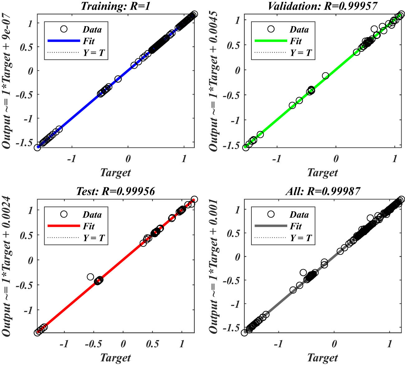
Statistical analysis with data from
According to Tables 1–4, the ANN algorithm outperformed the computational approaches in producing good outcomes. Previous research has shown that ANNs can reliably predict the rates of skin friction and heat transfer.
ANN and numerical method (NM) values of
|
|
|
|
|
|
|
||||
|---|---|---|---|---|---|---|---|---|---|
| NM | ANN | Error | NM | ANN | Error | ||||
| 0.2 | 0.1 | 2 | 0.5 | −1.28500 | −1.29336 | 8.35 × 10⁻³ | −0.44674 | −0.43955 | 7.19 × 10⁻³ |
| 0.4 | 0.1 | 2 | 0.5 | −1.36623 | −1.36676 | 5.26 × 10⁻⁴ | −0.42593 | −0.42535 | 5.84 × 10⁻⁴ |
| 0.6 | 0.1 | 2 | 0.5 | −1.42569 | −1.42570 | 1.51 × 10⁻⁵ | −0.41424 | −0.41442 | 1.89 × 10⁻⁴ |
| 0.8 | 0.1 | 2 | 0.5 | −1.47085 | −1.47085 | 9.47 × 10⁻⁷ | −0.40650 | −0.40666 | 1.61 × 10⁻⁴ |
| 1 | 0.1 | 2 | 0.5 | −1.50628 | −1.50625 | 2.69 × 10⁻⁵ | −0.40080 | −0.40067 | 1.33 × 10⁻⁴ |
| 0.5 | 0.1 | 2 | 0.5 | −1.39813 | −1.39812 | 1.01 × 10⁻⁵ | −0.41939 | −0.41943 | 4.64 × 10⁻⁵ |
| 0.5 | 0.2 | 2 | 0.5 | −1.42935 | −1.42975 | 3.99 × 10⁻⁴ | −0.40695 | −0.40672 | 2.28 × 10⁻⁴ |
| 0.5 | 0.3 | 2 | 0.5 | −1.46033 | −1.46048 | 1.55 × 10⁻⁴ | −0.39539 | −0.39503 | 3.64 × 10⁻⁴ |
| 0.5 | 0.4 | 2 | 0.5 | −1.49102 | −1.49090 | 1.15 × 10⁻⁴ | −0.38464 | −0.38440 | 2.42 × 10⁻⁴ |
| 0.5 | 0.5 | 2 | 0.5 | −1.52140 | −1.52150 | 1.00 × 10⁻⁴ | −0.37462 | −0.37483 | 2.09 × 10⁻⁴ |
| 0.5 | 0.1 | 0.5 | 0.5 | −1.22997 | −1.22984 | 1.29 × 10⁻⁴ | −0.47260 | −0.47243 | 1.67 × 10⁻⁴ |
| 0.5 | 0.1 | 1 | 0.5 | −1.28733 | −1.28756 | 2.22 × 10⁻⁴ | −0.45330 | −0.45369 | 3.85 × 10⁻⁴ |
| 0.5 | 0.1 | 1.5 | 0.5 | −1.34339 | −1.34500 | 1.60 × 10⁻³ | −0.43560 | −0.43597 | 3.73 × 10⁻⁴ |
| 0.5 | 0.1 | 2.5 | 0.5 | −1.45155 | −1.45153 | 1.73 × 10⁻⁵ | −0.40453 | −0.40480 | 2.67 × 10⁻⁴ |
| 0.5 | 0.1 | 2 | 0.2 | −1.34199 | −1.34179 | 1.95 × 10⁻⁴ | −0.17827 | −0.17845 | 1.86 × 10⁻⁴ |
| 0.5 | 0.1 | 2 | 0.4 | −1.37593 | −1.37680 | 8.69 × 10⁻⁴ | −0.34343 | −0.34231 | 1.12 × 10⁻³ |
| 0.5 | 0.1 | 2 | 0.6 | −1.42255 | −1.42281 | 2.52 × 10⁻⁴ | −0.49097 | −0.49034 | 6.36 × 10⁻⁴ |
| 0.5 | 0.1 | 2 | 0.8 | −1.47550 | −1.48506 | 9.56 × 10⁻³ | −0.62229 | −0.61223 | 1.01 × 10⁻² |
| 0.5 | 0.1 | 2 | 1 | −1.53115 | −1.55502 | 2.39 × 10⁻² | −0.74025 | −0.71106 | 2.92 × 10⁻² |
ANN and NM values of
|
|
|
|
|
|
|
|
|
||
|---|---|---|---|---|---|---|---|---|---|
| NM | ANN | Error | |||||||
| 0.5 | 1 | 1 | 0.5 | 1 | 0.2 | 0.2 | 1.123029 | 1.122525 | 5.04 × 10⁻⁴ |
| 0.7 | 1 | 1 | 0.5 | 1 | 0.2 | 0.2 | 1.063285 | 1.064012 | 7.27 × 10⁻⁴ |
| 0.9 | 1 | 1 | 0.5 | 1 | 0.2 | 0.2 | 1.010646 | 1.011047 | 4.00 × 10⁻⁴ |
| 1.1 | 1 | 1 | 0.5 | 1 | 0.2 | 0.2 | 0.96383 | 0.963699 | 1.30 × 10⁻⁴ |
| 1.3 | 1 | 1 | 0.5 | 1 | 0.2 | 0.2 | 0.921836 | 0.921834 | 2.46 × 10⁻⁶ |
| 1 | 0.2 | 1 | 0.5 | 1 | 0.2 | 0.2 | 1.111102 | 1.110997 | 1.05 × 10⁻⁴ |
| 1 | 0.3 | 1 | 0.5 | 1 | 0.2 | 0.2 | 1.095564 | 1.095749 | 1.86 × 10⁻⁴ |
| 1 | 0.4 | 1 | 0.5 | 1 | 0.2 | 0.2 | 1.080018 | 1.080167 | 1.49 × 10⁻⁴ |
| 1 | 0.5 | 1 | 0.5 | 1 | 0.2 | 0.2 | 1.064465 | 1.064394 | 7.04 × 10⁻⁵ |
| 1 | 0.6 | 1 | 0.5 | 1 | 0.2 | 0.2 | 1.048903 | 1.048562 | 3.42 × 10⁻⁴ |
| 1 | 1 | 0.2 | 0.5 | 1 | 0.2 | 0.2 | 1.113345 | 1.113623 | 2.78 × 10⁻⁴ |
| 1 | 1 | 0.3 | 0.5 | 1 | 0.2 | 0.2 | 1.098184 | 1.098261 | 7.66 × 10⁻⁵ |
| 1 | 1 | 0.4 | 0.5 | 1 | 0.2 | 0.2 | 1.082842 | 1.082799 | 4.35 × 10⁻⁵ |
| 1 | 1 | 0.5 | 0.5 | 1 | 0.2 | 0.2 | 1.067312 | 1.067215 | 9.68 × 10⁻⁵ |
| 1 | 1 | 0.6 | 0.5 | 1 | 0.2 | 0.2 | 1.051587 | 1.051489 | 9.86 × 10⁻⁵ |
| 1 | 1 | 1 | 0.2 | 1 | 0.2 | 0.2 | 0.651795 | 0.815917 | 1.64 × 10⁻¹ |
| 1 | 1 | 1 | 0.3 | 1 | 0.2 | 0.2 | 0.790207 | 0.864505 | 7.43 × 10⁻² |
| 1 | 1 | 1 | 0.4 | 1 | 0.2 | 0.2 | 0.898218 | 0.921206 | 2.30 × 10⁻² |
| 1 | 1 | 1 | 0.5 | 1 | 0.2 | 0.2 | 0.986578 | 0.986675 | 9.64 × 10⁻⁵ |
| 1 | 1 | 1 | 0.6 | 1 | 0.2 | 0.2 | 1.061072 | 1.061072 | 4.66 × 10⁻⁷ |
| 1 | 1 | 1 | 0.5 | 0.1 | 0.2 | 0.2 | 1.213823 | 1.211967 | 1.86 × 10⁻³ |
| 1 | 1 | 1 | 0.5 | 0.2 | 0.2 | 0.2 | 1.184912 | 1.18449 | 4.22 × 10⁻⁴ |
| 1 | 1 | 1 | 0.5 | 0.3 | 0.2 | 0.2 | 1.156972 | 1.157182 | 2.11 × 10⁻⁴ |
| 1 | 1 | 1 | 0.5 | 0.4 | 0.2 | 0.2 | 1.129979 | 1.130291 | 3.12 × 10⁻⁴ |
| 1 | 1 | 1 | 0.5 | 0.5 | 0.2 | 0.2 | 1.103912 | 1.104025 | 1.14 × 10⁻⁴ |
| 1 | 1 | 1 | 0.5 | 1 | 0.05 | 0.2 | 1.083454 | 1.083309 | 1.45 × 10⁻⁴ |
| 1 | 1 | 1 | 0.5 | 1 | 0.1 | 0.2 | 1.050012 | 1.050340 | 3.28 × 10⁻⁴ |
| 1 | 1 | 1 | 0.5 | 1 | 0.15 | 0.2 | 1.017731 | 1.017488 | 2.43 × 10⁻⁴ |
| 1 | 1 | 1 | 0.5 | 1 | 0.2 | 0.2 | 0.986578 | 0.986675 | 9.64 × 10⁻⁵ |
| 1 | 1 | 1 | 0.5 | 1 | 0.25 | 0.2 | 0.956518 | 0.959041 | 2.52 × 10⁻³ |
| 1 | 1 | 1 | 0.5 | 1 | 0.2 | 0.05 | 1.139136 | 1.139144 | 8.50 × 10⁻⁶ |
| 1 | 1 | 1 | 0.5 | 1 | 0.2 | 0.1 | 1.086488 | 1.086492 | 4.29 × 10⁻⁶ |
| 1 | 1 | 1 | 0.5 | 1 | 0.2 | 0.15 | 1.035641 | 1.035751 | 1.10 × 10⁻⁴ |
| 1 | 1 | 1 | 0.5 | 1 | 0.2 | 0.2 | 0.986578 | 0.986675 | 9.64 × 10⁻⁵ |
| 1 | 1 | 1 | 0.5 | 1 | 0.2 | 0.25 | 0.939281 | 0.939489 | 2.08 × 10⁻⁴ |
ANN and NM values of
|
|
|
|
|
|
n1 |
|
||
|---|---|---|---|---|---|---|---|---|
| NM | ANN | Error | ||||||
| 0.2 | 0.5 | 1.5 | 1 | 0.5 | 0.5 | −0.556680 | −0.340330 | 2.16 × 10⁻¹ |
| 0.4 | 0.5 | 1.5 | 1 | 0.5 | 0.5 | −0.176150 | -0.119010 | 5.71 × 10⁻² |
| 0.6 | 0.5 | 1.5 | 1 | 0.5 | 0.5 | 0.109308 | 0.109317 | 9.25 × 10⁻⁶ |
| 0.8 | 0.5 | 1.5 | 1 | 0.5 | 0.5 | 0.341719 | 0.332926 | 8.79 × 10⁻³ |
| 1 | 0.5 | 1.5 | 1 | 0.5 | 0.5 | 0.540186 | 0.540122 | 6.44 × 10⁻⁵ |
| 1 | 0.2 | 1.5 | 1 | 0.5 | 0.5 | 0.399204 | 0.402061 | 2.86 × 10⁻³ |
| 1 | 0.4 | 1.5 | 1 | 0.5 | 0.5 | 0.495065 | 0.495306 | 2.40 × 10⁻⁴ |
| 1 | 0.6 | 1.5 | 1 | 0.5 | 0.5 | 0.583659 | 0.583609 | 5.02 × 10⁻⁵ |
| 1 | 0.8 | 1.5 | 1 | 0.5 | 0.5 | 0.666208 | 0.666407 | 1.99 × 10⁻⁴ |
| 1 | 1 | 1.5 | 1 | 0.5 | 0.5 | 0.743640 | 0.743583 | 5.72 × 10⁻⁵ |
| 1 | 0.5 | 0.5 | 1 | 0.5 | 0.5 | 0.425713 | 0.425475 | 2.38 × 10⁻⁴ |
| 1 | 0.5 | 1 | 1 | 0.5 | 0.5 | 0.484723 | 0.485345 | 6.22 × 10⁻⁴ |
| 1 | 0.5 | 1.5 | 1 | 0.5 | 0.5 | 0.540186 | 0.540122 | 6.44 × 10⁻⁵ |
| 1 | 0.5 | 2 | 1 | 0.5 | 0.5 | 0.590057 | 0.589959 | 9.73 × 10⁻⁵ |
| 1 | 0.5 | 2.5 | 1 | 0.5 | 0.5 | 0.634937 | 0.635058 | 1.21 × 10⁻⁴ |
| 1 | 0.5 | 1.5 | 0.5 | 0.5 | 0.5 | 0.645172 | 0.644991 | 1.82 × 10⁻⁴ |
| 1 | 0.5 | 1.5 | 0.6 | 0.5 | 0.5 | 0.621603 | 0.621791 | 1.88 × 10⁻⁴ |
| 1 | 0.5 | 1.5 | 0.7 | 0.5 | 0.5 | 0.599363 | 0.599529 | 1.66 × 10⁻⁴ |
| 1 | 0.5 | 1.5 | 0.8 | 0.5 | 0.5 | 0.578410 | 0.578376 | 3.46 × 10⁻⁵ |
| 1 | 0.5 | 1.5 | 0.9 | 0.5 | 0.5 | 0.558700 | 0.558511 | 1.90 × 10⁻⁴ |
| 1 | 0.5 | 1.5 | 1 | 0.2 | 0.5 | 0.354393 | 0.354404 | 1.13 × 10⁻⁵ |
| 1 | 0.5 | 1.5 | 1 | 0.4 | 0.5 | 0.495255 | 0.495489 | 2.34 × 10⁻⁴ |
| 1 | 0.5 | 1.5 | 1 | 0.6 | 0.5 | 0.575585 | 0.575873 | 2.88 × 10⁻⁴ |
| 1 | 0.5 | 1.5 | 1 | 0.8 | 0.5 | 0.627909 | 0.629297 | 1.39 × 10⁻³ |
| 1 | 0.5 | 1.5 | 1 | 1 | 0.5 | 0.664793 | 0.664781 | 1.27 × 10⁻⁵ |
ANN and NM values of
|
|
|
|
|
||
|---|---|---|---|---|---|
| NM | ANN | Error | |||
| 0.1 | 0.1 | 0.5 | 0.186948 | 0.186172 | 7.76 × 10⁻⁴ |
| 0.3 | 0.1 | 0.5 | 0.266109 | 0.267456 | 1.35 × 10⁻³ |
| 0.5 | 0.1 | 0.5 | 0.351812 | 0.351661 | 1.50 × 10⁻⁴ |
| 0.7 | 0.1 | 0.5 | 0.435993 | 0.435221 | 7.72 × 10⁻⁴ |
| 0.9 | 0.1 | 0.5 | 0.515392 | 0.515152 | 2.41 × 10⁻⁴ |
| 1 | 0.2 | 0.5 | 0.621191 | 0.619026 | 2.16 × 10⁻³ |
| 1 | 0.3 | 0.5 | 0.689628 | 0.687994 | 1.63 × 10⁻³ |
| 1 | 0.4 | 0.5 | 0.758395 | 0.758442 | 4.65 × 10⁻⁵ |
| 1 | 0.5 | 0.5 | 0.827481 | 0.828669 | 1.19 × 10⁻³ |
| 1 | 0.6 | 0.5 | 0.896875 | 0.896838 | 3.75 × 10⁻⁵ |
| 1 | 0.1 | 0.2 | 0.539954 | 0.539980 | 2.61 × 10⁻⁵ |
| 1 | 0.1 | 0.3 | 0.544334 | 0.544349 | 1.46 × 10⁻⁵ |
| 1 | 0.1 | 0.4 | 0.548715 | 0.548725 | 1.03 × 10⁻⁵ |
| 1 | 0.1 | 0.5 | 0.553095 | 0.553127 | 3.23 × 10⁻⁵ |
| 1 | 0.1 | 0.6 | 0.557475 | 0.557576 | 1.01 × 10⁻⁴ |
5 Findings and analysis
The purpose of this section is to show how the activation energy and Coriolis force affect the flow of a DF containing gyrotactic microbes over a three-dimensional surface. In this part, we look at the dusty and hybrid phases and how momentum and thermal characteristics are physically important. It also explores the key elements that affect the velocity of DNFs, including gyrotactic microorganisms.
Comparison of
|
|
Rehman et al. [42] | Ali et al. [43] | Present |
|---|---|---|---|
| 1.0 | 1.00000 | 1.0000 | 1.00000 |
| 3.0 | 1.92375 | 1.9236 | 1.92375 |
| 10 | 3.72061 | 3.7207 | 3.72061 |
| 100 | 12.29404 | 12.294 | 12.29404 |
5.1 Effect of fluid–particle interaction
(
β
v
)
Figure 5(a–d) depicts how the fluid–particle interaction parameter

Influence of
5.2 Effect of porosity
(
ϒ
)
Figure 6(a–d) describes variations in the velocities

Influence of
5.3 Effect of mass concentration of dust particles
(
I
)
The impact of

Influence of
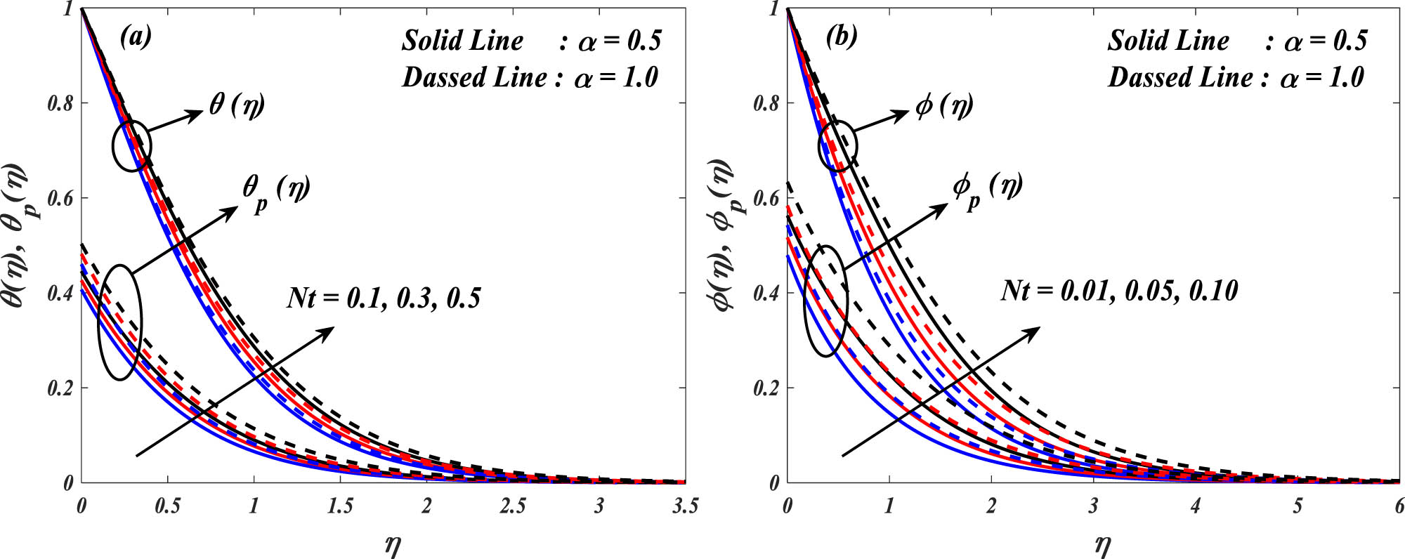
5.4 Effect of thermophoresis
(
Nt
)
The impact of the
Influence of
5.5 Effect of Brownian motion
(
Nb
)
The Brownian motion parameter’s

Influence of
5.6 Effect of specific heat ratio
(
γ
)
Figure 10(a and b) explores the effect of changes in

Influence of
The same nature is observed for the concentration profile
5.7 Effects of radiation
(
Rd
)
and accumulation
(
A
)
&
(
B
)
Figure 11 demonstrates the influence of the radiation parameter (Rd) on the temperature profiles of the fluid and dusty phases. The graph presented here indicates that the temperature

Influence of

Influence of

Influence of
5.8 Effect of fluid–particle interaction
(
β
t
)
Figure 14 displays the variations in the temperature profile

Influence of
5.9 Effect of fluid–particle interaction
(
E
)
Figure 15 demonstrates how the activation energy parameter

Influence of
5.10 Effect of chemical reaction
(
Γ
)
Various values of the chemical reaction parameter

Influence of
5.11 Effect of fluid–particle interaction
(
β
c
)
Figure 17 shows the concentration profile

Influence of
5.12 Effect of Peclet number
(
Pe
)
An illustration of the effect that the Peclet number

Influence of
5.13 Effect of microorganism density
(
χ
w
)
The influence of microorganism density

Influence of
5.14 Effect of skin friction
(
C
A
x
Re
x
1
/
2
)
&
(
C
A
y
Re
x
1
/
2
)
, Nusselt number
(
Nu
Re
x
−
1
/
2
)
, mass transfer rate
(
Sh
Re
x
−
1
/
2
)
, and motile microorganism
Figure 20(a–e) is shown in order to demonstrate the impact of the fluid–particle interaction parameter

Influence of

Influence of

Influence of
6 Conclusion
This study demonstrates the efficacy of a multi-layer ANN in analyzing the effects of the Coriolis force and activation energy on the flow of a DNF containing gyrotactic microorganisms over a three-dimensional sheet. The study also considers the influence of linear thermal radiation and a non-uniform heat source on the system. The results are presented in two-dimensional graphs, revealing the following key findings:
The ANN methodology effectively reduces computational time when solving complex fluid dynamics problems.
The dust fluid velocity
The temperature
Higher values of the thermophoresis parameter
An increase in the Brownian motion parameter
The microorganism density
The rate of heat transfer
The findings have practical implications in geothermal energy extraction, industrial cooling systems, wastewater treatment, and enhanced oil recovery. For instance, in geothermal power plants, optimizing nanofluid properties can improve heat transfer efficiency, reducing energy consumption. Similarly, in wastewater treatment, understanding microorganism dynamics helps in bacterial control, improving purification efficiency. These insights contribute to sustainable and efficient thermal management solutions across industries. Future investigations may include hybrid nanofluids, magnetohydrodynamic effects, and experimental validation using CFDs and deep learning. Current constraints include constant property assumptions, nanoparticle aggregation, and the lack of empirical validation.
Acknowledgments
This work was supported by the Government wide R&D Fund Infectious Disease Research (GFID), with a grant funded by the government of the Republic of Korea (Ministry of Health and welfare), Korea Health Industry Development Institute (KHIDI) (The development of infection control and prevention technologies for strengthening the infection control capacity of medical institutions), under Grant RS-2025-02310471.
-
Funding information: This work was supported by the Government wide R&D Fund Infectious Disease Research (GFID), with a grant funded by the government of the Republic of Korea (Ministry of Health and welfare), Korea Health Industry Development Institute (KHIDI) (The development of infection control and prevention technologies for strengthening the infection control capacity of medical institutions), under Grant RS-2025-02310471.
-
Author contributions: All authors have accepted responsibility for the entire content of this manuscript and approved its submission.
-
Conflict of interest: The authors state no conflict of interest.
-
Data availability statement: All data generated or analyzed in this study are fully presented within this published article.
References
[1] Rashed AS, Mahmoud TA, Mabrouk SM. Enhanced flow and temperature profiles in ternary hybrid nanofluid with gyrotactic microorganisms: a study on magnetic field, brownian motion, and thermophoresis phenomena. J Appl Comput Mech. 2024;10:597–609. 10.22055/jacm.2024.45899.4427.Suche in Google Scholar
[2] Atif SM, Hussain S, Sagheer M. Magnetohydrodynamic stratified bioconvective flow of micropolar nanofluid due to gyrotactic microorganisms. AIP Adv. 2019;9:025208. 10.1063/1.5085742.Suche in Google Scholar
[3] Begum N, Siddiqa S, Sulaiman M, Islam S, Hossain MA, Gorla RSR. Numerical solutions for gyrotactic bioconvection of dusty nanofluid along a vertical isothermal surface. Int J Heat Mass Transf. 2017;113:229–36. 10.1016/j.ijheatmasstransfer.2017.05.071.Suche in Google Scholar
[4] Agarwal P, Jain R, Loganathan K. Thermally radiative flow of MHD Powell-Eyring nanofluid over an exponential stretching sheet with swimming microorganisms and viscous dissipation: A numerical computation. Int J Thermofluids. 2024;23:100773. 10.1016/j.ijft.2024.100773.Suche in Google Scholar
[5] Rajeswari PM, De P. Multi-stratified effects on stagnation point nanofluid flow with gyrotactic microorganisms over porous medium. J Porous Media. 2024;27:67–84. 10.1615/JPorMedia.2023050040.Suche in Google Scholar
[6] Jakeer S, Polu BAR. Homotopy perturbation method solution of magneto-polymer nanofluid containing gyrotactic microorganisms over the permeable sheet with Cattaneo–Christov heat and mass flux model. Proc Inst Mech Eng Part E J Process Mech Eng. 2021;236:525–34. 10.1177/09544089211048993.Suche in Google Scholar
[7] Basha HT, Sivaraj R. Numerical simulation of blood nanofluid flow over three different geometries by means of gyrotactic microorganisms: Applications to the flow in a circulatory system. Proc Inst Mech Eng Part C J Mech Eng Sci. 2021;235:441–60. 10.1177/0954406220947454.Suche in Google Scholar
[8] Alharbi FM, Naeem M, Zubair M, Jawad M, Jan WU, Jan R. Bioconvection due to gyrotactic microorganisms in couple stress hybrid nanofluid laminar mixed convection incompressible flow with magnetic nanoparticles and chemical reaction as carrier for targeted drug delivery through porous stretching sheet. Molecules. 2021;26:3954. 10.3390/molecules26133954.Suche in Google Scholar PubMed PubMed Central
[9] Waqas H, Kamran T, Imran M, Muhammad T. MHD bioconvectional flow of Jeffrey nanofluid with motile microorganisms over a stretching sheet: solar radiation applications. Waves Random Complex Media. 2022;1–30. 10.1080/17455030.2022.2105418.Suche in Google Scholar
[10] Mehmood Z, Iqbal Z. Interaction of induced magnetic field and stagnation point flow on bioconvection nanofluid submerged in gyrotactic microorganisms. J Mol Liq. 2016;224:1083–91. 10.1016/j.molliq.2016.10.014.Suche in Google Scholar
[11] Kuznetsov AV. The onset of nanofluid bioconvection in a suspension containing both nanoparticles and gyrotactic microorganisms. Int Commun Heat Mass Transf. 2010;37:1421–5. 10.1016/j.icheatmasstransfer.2010.08.015.Suche in Google Scholar
[12] Ahmad S, Akhter S, Imran Shahid M, Ali K, Akhtar M, Ashraf M. Novel thermal aspects of hybrid nanofluid flow comprising of manganese zinc ferrite MnZnFe2O4, nickel zinc ferrite NiZnFe2O4 and motile microorganisms. Ain Shams Eng J. 2022;13:101668. 10.1016/j.asej.2021.101668.Suche in Google Scholar
[13] Dey D, Chutia B. Dusty nanofluid flow with bioconvection past a vertical stretching surface. J King Saud Univ – Eng Sci. 2022;34:375–80. 10.1016/j.jksues.2020.11.001.Suche in Google Scholar
[14] Rajeswari PM, De P. Shape factor and sensitivity analysis on stagnation point of bioconvective tetra-hybrid nanofluid over porous stretched vertical cylinder. Bionanoscience. 2024;14:3035–58. 10.1007/s12668-024-01586-8.Suche in Google Scholar
[15] Loganathan K, Jain R, Eswaramoorthi S, Abbas M, Alqahtani MS. Bioconvective gyrotactic microorganisms in third-grade nanofluid flow over a Riga surface with stratification: An approach to entropy minimization. Open Phys. 2023;21:20230273. 10.1515/phys-2023-0273.Suche in Google Scholar
[16] Loganathan K, Alessa N, Jain R, Ali F, Zaib A. Dynamics of heat and mass transfer: Ree-Eyring nanofluid flow over a Riga plate with bioconvention and thermal radiation. Front Phys. 2022;10:974562. 10.3389/fphy.2022.974562.Suche in Google Scholar
[17] Rashed AS, Nasr E, Mabrouk SM. Bioconvective flow surrounding a thin surgical needle in blood incorporating ternary hybrid nanoparticles. Comput Methods Differ Equations. 2024. 10.22034/CMDE.2024.61425.2643.Suche in Google Scholar
[18] Fortov VE, Vaulina OS, Petrov OF, Vasiliev MN, Gavrikov AV, Shakova IA, et al. Experimental study of the heat transport processes in dusty plasma fluid. Phys Rev E – Stat Nonlinear, Soft Matter Phys. 2007;75:026403. 10.1103/PhysRevE.75.026403.Suche in Google Scholar PubMed
[19] Basha HT, Kim H, Jang B. Buoyancy-driven heat transfer and entropy analysis of a hydromagnetic GO-Fe3O4/H2O hybrid nanofluid in an energy storage enclosure partially filled with non-Darcy porous medium under an oblique magnetic field. Int J Numer Methods Heat Fluid Flow. 2024;35:491–523. 10.1108/HFF-03-2024-0193/FULL/XML.Suche in Google Scholar
[20] Basha HT, Jang B. Machine learning analysis for heat transfer enhancement in nano-encapsulated phase change materials within L-shaped enclosure with heated blocks. Appl Therm Eng. 2025;259:124803. 10.1016/J.APPLTHERMALENG.2024.124803.Suche in Google Scholar
[21] Jakeer S, Reddy PBA. Entropy generation on the variable magnetic field and magnetohydrodynamic stagnation point flow of Eyring–Powell hybrid dusty nanofluid: Solar thermal application. Proc Inst Mech Eng Part C J Mech Eng Sci. 2022;236:7442–55. 10.1177/09544062211072457.Suche in Google Scholar
[22] Lou Q, Ali B, Rehman SU, Habib D, Abdal S, Shah NA, et al. Micropolar dusty fluid: Coriolis force effects on dynamics of MHD rotating fluid when Lorentz force is significant. Mathematics. 2022;10:1–13. 10.3390/math10152630.Suche in Google Scholar
[23] Kalpana G, Madhura KR, Kudenatti RB. Impact of temperature-dependant viscosity and thermal conductivity on MHD boundary layer flow of two-phase dusty fluid through permeable medium. Eng Sci Technol Int J. 2019;22:416–27. 10.1016/j.jestch.2018.10.009.Suche in Google Scholar
[24] Mahdy A, Hoshoudy GA. Two-phase mixed convection nanofluid flow of a dusty tangent hyperbolic past a nonlinearly stretching sheet. J Egypt Math Soc. 2019;27:44. 10.1186/s42787-019-0050-9.Suche in Google Scholar
[25] Ramana Reddy JV, Sugunamma V, Sandeep N. Thermophoresis and Brownian motion effects on unsteady MHD nanofluid flow over a slendering stretching surface with slip effects. Alex Eng J. 2018;57:2465–73. 10.1016/j.aej.2017.02.014.Suche in Google Scholar
[26] Ghadikolaei SS, Hosseinzadeh K, Hatami M, Ganji DD. MHD boundary layer analysis for micropolar dusty fluid containing Hybrid nanoparticles (Cu‑Al2O3) over a porous medium. J Mol Liq. 2018;268:813–23. 10.1016/J.MOLLIQ.2018.07.105.Suche in Google Scholar
[27] Gnaneswara Reddy M, Sudha Rani MVVNL, Ganesh Kumar K, Prasannakumar BC, Lokesh HJ. Hybrid dusty fluid flow through a Cattaneo–Christov heat flux model. Phys A Stat Mech Its Appl. 2020;511:123975. 10.1016/j.physa.2019.123975.Suche in Google Scholar
[28] Imitaz A, Aamina A, Ali F, Khan I, Nisar KS. Two-phase flow of blood with magnetic dusty particles in cylindrical region: A Caputo-Fabrizio fractional model. Comput Mater Contin. 2020;66:2253–64. 10.32604/cmc.2021.012470.Suche in Google Scholar
[29] Nawaz M, Madkhali HA, Haneef M, Alharbi SO, Alaoui MK. Numerical study on thermal enhancement in hyperbolic tangent fluid with dust and hybrid nanoparticles. Int Commun Heat Mass Transf. 2021;127:105535. 10.1016/j.icheatmasstransfer.2021.105535.Suche in Google Scholar
[30] De MA. Comparative study of hybrid, tri-hybrid and tetra-hybrid nanoparticles in MHD unsteady flow with chemical reaction, activation energy, Soret-Dufour effect and sensitivity analysis over non-Darcy porous stretching cylinder. Heliyon. 2024;10:e35731. 10.1016/j.heliyon.2024.e35731.Suche in Google Scholar PubMed PubMed Central
[31] Khan MI, Hayat T, Khan MI, Alsaedi A. Activation energy impact in nonlinear radiative stagnation point flow of cross nanofluid. Int Commun Heat Mass Transf. 2018;91:216–24. 10.1016/j.icheatmasstransfer.2017.11.001.Suche in Google Scholar
[32] Hayat T, Riaz R, Aziz A, Alsaedi A. Influence of Arrhenius activation energy in MHD flow of third grade nanofluid over a nonlinear stretching surface with convective heat and mass conditions. Phys A Stat Mech Appl. 2020;549:124006. 10.1016/j.physa.2019.124006.Suche in Google Scholar
[33] Lian W, Wang J, Wang G, Gao D, Li X, Zhang Z, et al. Investigation on the lignite pyrolysis reaction kinetics based on the general Arrhenius formula. Fuel. 2020;268:117364. 10.1016/j.fuel.2020.117364.Suche in Google Scholar
[34] Khan MI, Qayyum S, Hayat T, Waqas M, Imran M, Alsaedi A. Entropy generation minimization and binary chemical reaction with Arrhenius activation energy in MHD radiative flow of nanomaterial. J Mol Liq. 2018;259:274–83. 10.1016/j.molliq.2018.03.049.Suche in Google Scholar
[35] Khan MI, Ahmad MW, Alsaedi A, Hayat T. Entropy generation optimization in flow of non-Newtonian nanomaterial with binary chemical reaction and Arrhenius activation energy. Phys A. 2020;538:122806. 10.1016/j.physa.2019.122806.Suche in Google Scholar
[36] Shafique Z, Mustafa M, Mushtaq A. Boundary layer flow of Maxwell fluid in rotating frame with binary chemical reaction and activation energy. Results Phys. 2016;6:627–33. 10.1016/j.rinp.2016.09.006.Suche in Google Scholar
[37] Reddy SRR, Bala Anki Reddy P, Bhattacharyya K. Effect of nonlinear thermal radiation on 3D magneto slip flow of Eyring-Powell nanofluid flow over a slendering sheet with binary chemical reaction and Arrhenius activation energy. Adv Powder Technol. 2019;30:3203–13. 10.1016/j.apt.2019.09.029.Suche in Google Scholar
[38] Gomathi N, Poulomi D. Dual solutions of Casson Williamson nanofluid with thermal radiation and chemical reaction. Numer Heat Transf Part A Appl. 2024;1–24. 10.1080/10407782.2024.2326980.Suche in Google Scholar
[39] Mabrouk SM, Inc M, Rashed AS, Akgül A. Similarity analysis of bioconvection of unsteady nonhomogeneous hybrid nanofluids influenced by motile microorganisms. J Biol Phys. 2024;50:119–48. 10.1007/s10867-023-09651-1.Suche in Google Scholar PubMed PubMed Central
[40] Reddy SRR, Jakeer S, Rupa ML. ANN model of three-dimensional micropolar dusty hybrid nanofluid flow with Coriolis force: biomedical applications. Indian J Phys. 2023;97:3801–25. 10.1007/s12648-023-02737-5.Suche in Google Scholar
[41] Jakeer S, Rupa ML, Reddy SRR, Rashad AM. Artificial neural network model of non-Darcy MHD Sutterby hybrid nanofluid flow over a curved permeable surface: Solar energy applications. Propuls Power Res. 2023;12:410–27. 10.1016/j.jppr.2023.07.002.Suche in Google Scholar
[42] Rehman SU, Mariam A, Ullah A, Asjad MI, Bajuri MY, Pansera BA, et al. Numerical computation of buoyancy and radiation effects on MHD micropolar nanofluid flow over a stretching/shrinking sheet with heat source. Case Stud Therm Eng. 2021;25:100867. 10.1016/J.CSITE.2021.100867.Suche in Google Scholar
[43] Ali B, Nie Y, Khan SA, Sadiq MT, Tariq M. Finite element simulation of multiple slip effects on MHD unsteady Maxwell nanofluid flow over a permeable stretching sheet with radiation and thermo-diffusion in the presence of chemical reaction. Processes. 2019;7:628. 10.3390/PR7090628.Suche in Google Scholar
© 2025 the author(s), published by De Gruyter
This work is licensed under the Creative Commons Attribution 4.0 International License.
Artikel in diesem Heft
- Research Articles
- MHD radiative mixed convective flow of a sodium alginate-based hybrid nanofluid over a convectively heated extending sheet with Joule heating
- Experimental study of mortar incorporating nano-magnetite on engineering performance and radiation shielding
- Multicriteria-based optimization and multi-variable non-linear regression analysis of concrete containing blends of nano date palm ash and eggshell powder as cementitious materials
- A promising Ag2S/poly-2-amino-1-mercaptobenzene open-top spherical core–shell nanocomposite for optoelectronic devices: A one-pot technique
- Biogenic synthesized selenium nanoparticles combined chitosan nanoparticles controlled lung cancer growth via ROS generation and mitochondrial damage pathway
- Fabrication of PDMS nano-mold by deposition casting method
- Stimulus-responsive gradient hydrogel micro-actuators fabricated by two-photon polymerization-based 4D printing
- Physical aspects of radiative Carreau nanofluid flow with motile microorganisms movement under yield stress via oblique penetrable wedge
- Effect of polar functional groups on the hydrophobicity of carbon nanotubes-bacterial cellulose nanocomposite
- Review in green synthesis mechanisms, application, and future prospects for Garcinia mangostana L. (mangosteen)-derived nanoparticles
- Entropy generation and heat transfer in nonlinear Buoyancy–driven Darcy–Forchheimer hybrid nanofluids with activation energy
- Green synthesis of silver nanoparticles using Ginkgo biloba seed extract: Evaluation of antioxidant, anticancer, antifungal, and antibacterial activities
- A numerical analysis of heat and mass transfer in water-based hybrid nanofluid flow containing copper and alumina nanoparticles over an extending sheet
- Investigating the behaviour of electro-magneto-hydrodynamic Carreau nanofluid flow with slip effects over a stretching cylinder
- Electrospun thermoplastic polyurethane/nano-Ag-coated clear aligners for the inhibition of Streptococcus mutans and oral biofilm
- Investigation of the optoelectronic properties of a novel polypyrrole-multi-well carbon nanotubes/titanium oxide/aluminum oxide/p-silicon heterojunction
- Novel photothermal magnetic Janus membranes suitable for solar water desalination
- Green synthesis of silver nanoparticles using Ageratum conyzoides for activated carbon compositing to prepare antimicrobial cotton fabric
- Activation energy and Coriolis force impact on three-dimensional dusty nanofluid flow containing gyrotactic microorganisms: Machine learning and numerical approach
- Machine learning analysis of thermo-bioconvection in a micropolar hybrid nanofluid-filled square cavity with oxytactic microorganisms
- Research and improvement of mechanical properties of cement nanocomposites for well cementing
- Thermal and stability analysis of silver–water nanofluid flow over unsteady stretching sheet under the influence of heat generation/absorption at the boundary
- Cobalt iron oxide-infused silicone nanocomposites: Magnetoactive materials for remote actuation and sensing
- Magnesium-reinforced PMMA composite scaffolds: Synthesis, characterization, and 3D printing via stereolithography
- Bayesian inference-based physics-informed neural network for performance study of hybrid nanofluids
- Numerical simulation of non-Newtonian hybrid nanofluid flow subject to a heterogeneous/homogeneous chemical reaction over a Riga surface
- Enhancing the superhydrophobicity, UV-resistance, and antifungal properties of natural wood surfaces via in situ formation of ZnO, TiO2, and SiO2 particles
- Synthesis and electrochemical characterization of iron oxide/poly(2-methylaniline) nanohybrids for supercapacitor application
- Impacts of double stratification on thermally radiative third-grade nanofluid flow on elongating cylinder with homogeneous/heterogeneous reactions by implementing machine learning approach
- Synthesis of Cu4O3 nanoparticles using pumpkin seed extract: Optimization, antimicrobial, and cytotoxicity studies
- Cationic charge influence on the magnetic response of the Fe3O4–[Me2+ 1−y Me3+ y (OH2)] y+(Co3 2−) y/2·mH2O hydrotalcite system
- Pressure sensing intelligent martial arts short soldier combat protection system based on conjugated polymer nanocomposite materials
- Magnetohydrodynamics heat transfer rate under inclined buoyancy force for nano and dusty fluids: Response surface optimization for the thermal transport
- Fly ash and nano-graphene enhanced stabilization of engine oil-contaminated soils
- Enhancing natural fiber-reinforced biopolymer composites with graphene nanoplatelets: Mechanical, morphological, and thermal properties
- Performance evaluation of dual-scale strengthened co-bonded single-lap joints using carbon nanotubes and Z-pins with ANN
- Computational works of blood flow with dust particles and partially ionized containing tiny particles on a moving wedge: Applications of nanotechnology
- Hybridization of biocomposites with oil palm cellulose nanofibrils/graphene nanoplatelets reinforcement in green epoxy: A study of physical, thermal, mechanical, and morphological properties
- Design and preparation of micro-nano dual-scale particle-reinforced Cu–Al–V alloy: Research on the aluminothermic reduction process
- Spectral quasi-linearization and response optimization on magnetohydrodynamic flow via stenosed artery with hybrid and ternary solid nanoparticles: Support vector machine learning
- Ferrite/curcumin hybrid nanocomposite formulation: Physicochemical characterization, anticancer activity, and apoptotic and cell cycle analyses in skin cancer cells
- Enhanced therapeutic efficacy of Tamoxifen against breast cancer using extra virgin olive oil-based nanoemulsion delivery system
- A titanium oxide- and silver-based hybrid nanofluid flow between two Riga walls that converge and diverge through a machine-learning approach
- Enhancing convective heat transfer mechanisms through the rheological analysis of Casson nanofluid flow towards a stagnation point over an electro-magnetized surface
- Intrinsic self-sensing cementitious composites with hybrid nanofillers exhibiting excellent piezoresistivity
- Research on mechanical properties and sulfate erosion resistance of nano-reinforced coal gangue based geopolymer concrete
- Impact of surface and configurational features of chemically synthesized chains of Ni nanostars on the magnetization reversal process
- Porous sponge-like AsOI/poly(2-aminobenzene-1-thiol) nanocomposite photocathode for hydrogen production from artificial and natural seawater
- Multifaceted insights into WO3 nanoparticle-coupled antibiotics to modulate resistance in enteric pathogens of Houbara bustard birds
- Synthesis of sericin-coated silver nanoparticles and their applications for the anti-bacterial finishing of cotton fabric
- Enhancing chloride resistance of freeze–thaw affected concrete through innovative nanomaterial–polymer hybrid cementitious coating
- Development and performance evaluation of green aluminium metal matrix composites reinforced with graphene nanopowder and marble dust
- Morphological, physical, thermal, and mechanical properties of carbon nanotubes reinforced arrowroot starch composites
- Influence of the graphene oxide nanosheet on tensile behavior and failure characteristics of the cement composites after high-temperature treatment
- Central composite design modeling in optimizing heat transfer rate in the dissipative and reactive dynamics of viscoplastic nanomaterials deploying Joule and heat generation aspects
- Double diffusion of nano-enhanced phase change materials in connected porous channels: A hybrid ISPH-XGBoost approach
- Synergistic impacts of Thompson–Troian slip, Stefan blowing, and nonuniform heat generation on Casson nanofluid dynamics through a porous medium
- Optimization of abrasive water jet machining parameters for basalt fiber/SiO2 nanofiller reinforced composites
- Enhancing aesthetic durability of Zisha teapots via TiO2 nanoparticle surface modification: A study on self-cleaning, antimicrobial, and mechanical properties
- Nanocellulose solution based on iron(iii) sodium tartrate complexes
- Combating multidrug-resistant infections: Gold nanoparticles–chitosan–papain-integrated dual-action nanoplatform for enhanced antibacterial activity
- Novel royal jelly-mediated green synthesis of selenium nanoparticles and their multifunctional biological activities
- Direct bandgap transition for emission in GeSn nanowires
- Synthesis of ZnO nanoparticles with different morphologies using a microwave-based method and their antimicrobial activity
- Numerical investigation of convective heat and mass transfer in a trapezoidal cavity filled with ternary hybrid nanofluid and a central obstacle
- Halloysite nanotube enhanced polyurethane nanocomposites for advanced electroinsulating applications
- Low molar mass ionic liquid’s modified carbon nanotubes and its role in PVDF crystalline stress generation
- Green synthesis of polydopamine-functionalized silver nanoparticles conjugated with Ceftazidime: in silico and experimental approach for combating antibiotic-resistant bacteria and reducing toxicity
- Evaluating the influence of graphene nano powder inclusion on mechanical, vibrational and water absorption behaviour of ramie/abaca hybrid composites
- Dynamic-behavior of Casson-type hybrid nanofluids due to a stretching sheet under the coupled impacts of boundary slip and reaction-diffusion processes
- Influence of polyvinyl alcohol on the physicochemical and self-sensing properties of nano carbon black reinforced cement mortar
- Advanced machine learning approaches for predicting compressive and flexural strength of carbon nanotube–reinforced cement composites: a comparative study and model interpretability analysis
- Review Articles
- A comprehensive review on hybrid plasmonic waveguides: Structures, applications, challenges, and future perspectives
- Nanoparticles in low-temperature preservation of biological systems of animal origin
- Fluorescent sulfur quantum dots for environmental monitoring
- Nanoscience systematic review methodology standardization
- Nanotechnology revolutionizing osteosarcoma treatment: Advances in targeted kinase inhibitors
- AFM: An important enabling technology for 2D materials and devices
- Carbon and 2D nanomaterial smart hydrogels for therapeutic applications
- Principles, applications and future prospects in photodegradation systems
- Do gold nanoparticles consistently benefit crop plants under both non-stressed and abiotic stress conditions?
- An updated overview of nanoparticle-induced cardiovascular toxicity
- Arginine as a promising amino acid for functionalized nanosystems: Innovations, challenges, and future directions
- Advancements in the use of cancer nanovaccines: Comprehensive insights with focus on lung and colon cancer
- Membrane-based biomimetic delivery systems for glioblastoma multiforme therapy
- The drug delivery systems based on nanoparticles for spinal cord injury repair
- Green synthesis, biomedical effects, and future trends of Ag/ZnO bimetallic nanoparticles: An update
- Application of magnesium and its compounds in biomaterials for nerve injury repair
- Micro/nanomotors in biomedicine: Construction and applications
- Hydrothermal synthesis of biomass-derived CQDs: Advances and applications
- Research progress in 3D bioprinting of skin: Challenges and opportunities
- Review on bio-selenium nanoparticles: Synthesis, protocols, and applications in biomedical processes
- Gold nanocrystals and nanorods functionalized with protein and polymeric ligands for environmental, energy storage, and diagnostic applications: A review
- An in-depth analysis of rotational and non-rotational piezoelectric energy harvesting beams: A comprehensive review
- Advancements in perovskite/CIGS tandem solar cells: Material synergies, device configurations, and economic viability for sustainable energy
- Deep learning in-depth analysis of crystal graph convolutional neural networks: A new era in materials discovery and its applications
- Review of recent nano TiO2 film coating methods, assessment techniques, and key problems for scaleup
- Antioxidant quantum dots for spinal cord injuries: A review on advancing neuroprotection and regeneration in neurological disorders
- Rise of polycatecholamine ultrathin films: From synthesis to smart applications
- Advancing microencapsulation strategies for bioactive compounds: Enhancing stability, bioavailability, and controlled release in food applications
- Advances in the design and manipulation of self-assembling peptide and protein nanostructures for biomedical applications
- Photocatalytic pervious concrete systems: from classic photocatalysis to luminescent photocatalysis
- Corrigendum
- Corrigendum to “Synthesis and characterization of smart stimuli-responsive herbal drug-encapsulated nanoniosome particles for efficient treatment of breast cancer”
- Special Issue on Advanced Nanomaterials for Carbon Capture, Environment and Utilization for Energy Sustainability - Part III
- Efficiency optimization of quantum dot photovoltaic cell by solar thermophotovoltaic system
- Exploring the diverse nanomaterials employed in dental prosthesis and implant techniques: An overview
- Electrochemical investigation of bismuth-doped anode materials for low‑temperature solid oxide fuel cells with boosted voltage using a DC-DC voltage converter
- Synthesis of HfSe2 and CuHfSe2 crystalline materials using the chemical vapor transport method and their applications in supercapacitor energy storage devices
- Special Issue on Green Nanotechnology and Nano-materials for Environment Sustainability
- Influence of nano-silica and nano-ferrite particles on mechanical and durability of sustainable concrete: A review
- Surfaces and interfaces analysis on different carboxymethylation reaction time of anionic cellulose nanoparticles derived from oil palm biomass
- Processing and effective utilization of lignocellulosic biomass: Nanocellulose, nanolignin, and nanoxylan for wastewater treatment
- Retraction
- Retraction of “Aging assessment of silicone rubber materials under corona discharge accompanied by humidity and UV radiation”