Chaos and bifurcation in the controlled chaotic system

Yongjian Liu; Xiezhen Huang; Jincun Zheng

doi:10.1515/math-2018-0105

Article Open Access

Chaos and bifurcation in the controlled chaotic system

Yongjian Liu , Xiezhen Huang and Jincun Zheng

Published/Copyright: November 3, 2018

Published by

Become an author with De Gruyter Brill

Submit Manuscript Author Information Explore this Subject

$Open Mathematics$

From the journal Open Mathematics Volume 16 Issue 1

Abstract

In this paper, chaos and bifurcation are explored for the controlled chaotic system, which is put forward based on the hybrid strategy in an unusual chaotic system. Behavior of the controlled system with variable parameter is researched in detain. Moreover, the normal form theory is used to analyze the direction and stability of bifurcating periodic solution.

Keywords: Controlled chaotic system; Chaos; Bifurcation; Normal form theory

MSC 2010: 34C23; C34C28; C34C60; C34H20

1 Introduction

In 1963, the first three dimensional autonomous chaotic system (Lorenz system) was proposed in the literature [1]. After that, the construction and theoretical research of the chaotic system have become a hot issue in the nonlinear science. What is more, many three-dimensional chaotic systems have been put forward one after another, including Chen system [2] and Lu¨ system [3], which have to be mentioned. In the sense of literature [4], Chen system is the dual system of Lorenz system, whereas Lu¨system acts as a bridge between the both. In 1994, with the aid of a computer, Sprott has found 19 three-dimensional chaotic systems [5]. Ro¨ssler system [6] and Chua system [7] have also received widespread attention from scholars. More about the contents of chaotic systems can be seen in the literature [8, 9, 10, 11]. For most 3D systems, there may be only one equilibrium point, two symmetric equilibrium points, three equilibrium points or even more, their common features are that all of the equilibria are unstable [12]. In 2008, Yang and Chen [13] introduced a chaotic system [14] with a saddle point and two stable node-foci. Wei and Yang introduced a class of chaotic systems with only two stable equilibria [15]. In particular, the above mentioned chaotic systems have a common characteristic: the total stability of the two symmetric equilibria is always the same. Bifurcation analysis and control is one of the most popular research theme in the domain of bifurcation control [16, 17, 18, 19, 20, 21].

Liu et al. [22] gave a new 3D chaotic system as follows:

x˙=a(y−x),y˙=−c+xz,z˙=b−y2.

There are only two nonlinear terms on the right side of the system, which is simple, but the local dynamic behavior is complex and interesting. There is a pair of equilibrium points in the system, whose positions are symmetric but the stability is opposite. The nature of this new chaotic system has attracted extensive interest [23–26]. In this article, we design a hybrid strategy which consists of a parameter and a state feedback , and it is added to the last system, and we can get the controlled chaotic system as follows:

x˙=a(y−x),y˙=−c+xz+m(x−y),z˙=b−y2.

Apparently, this strategy not only ensures that the equilibrium structure and the dimension of the original system are unchanged. To analyze complex dynamical behaviors of the controlled system and evaluate differences of chaos between the original system and controlled system, we study the chaos and bifurcation of the controlled system through analyzing the variable parameter. First, phase trajectories, Lyapunove exponents and bifurcation path are numerically investigated. Chaotic area, period area and several periodic windows within the range of control parameter in controlled system are found. Then a sufficient condition for the existence of Hopf bifurcation of controlled system are given. The next theorem describes following details: the existence and expression of the bifurcation periodic solutions are explored, and the stability, direction and the period size also are studied.

The remainder of the article is arranged as follows: In section 2, hybrid control strategy of Hopf bifurcation is examined. In section 3, bifurcation diagrams and Lyapunov exponents of the controlled system with varying parameter m are analyzed in detail. The Hopf bifurcation and its periodic solution of the controlled system are explored in section 4. Finally, section 5 is summing up the full text.

2 Hybrid control strategy

For the convenience of description, the original system proposed in [22] as follows:

x˙=a(y−x)y˙=−c+xzz˙=b−y2,(2.1)

when parameters a(a > 0), b and c are all real constants, and x, y, z are three state variables in this case. Apparently, when c = 0, system (2.1) is invariant while it is under the transformation T(x, y, z) → T(−x, −y, z). In the sense of this transformation, the system not itself invariant under the T transformation, and there is another orbit that corresponds to it. We calculate the next formulas:

a(y−x)=0,−c+xz=0,b−y2=0.

a(y − x) = 0,−c + xz = 0, b − y₂ = 0.

It is easily obtained that if b₂ + c₂ = 0, there are non-isolated equilibria O_z(0,0, z); if either b < 0 or b = 0 and c ≠ 0, there is not an equilibrium; if b > 0, there are two equilibria E+(b,b,cb)andE−(−b,−b,−cb)..

In this part, based on the model (2.1), we design a controller to get the controlled system as below

x˙=a(y−x)y˙=−c+xz+m(x−y)z˙=b−y2.(2.2)

As needed, we only have to control the second equation, and the other two equations remain unchanged. Obviously, the characteristic of the control law is to ensure that the structure of the equilibrium and the dimension of the original system (2.1) are unchanged. Especially, if m = 0, the controlled system will restore to the original system.

The linearized system (2.2) acts at E_±, and we can get the Jacobian matrix

J±=−aa0m+z±−mx±0−2y±0,(2.3)

its characteristic equation being

Δ(λ)=λ3+(m+a)λ2+(2x±y±−az±)λ+2ax±y±=0.(2.4)

Regarding the controlled system, we conclude that if c>2bmba(a+m)E⁺ is unstable while E⁻ is stable, and if c<2bmba(a+m), E⁺ is stable while E⁻ is unstable. The stability of the both is always opposite.

We just analyse the stability of equilibrium E⁺. By using the Routh-Hurwitz criterion, we can easily prove the equilibrium E⁺ is stable while c<2bmba(a+m).

The formula (2.3) at equilibrium E⁺ is just as follows:

Δ+(λ)=λ3+(m+a)λ2+(2b−acb)λ+2ab=0.(2.5)

Let A=m+a,B=2b−acb,C=2ab. On the basis of the Routh-Hurwitz criterions, with the equation (2.4), while A > 0, C > 0, AB − C > 0, i.e. a > 0, b > 0, and c<2bmba(a+m), all of the real parts of the three roots are negative. We take into account the characteristic equation (2.3) at equilibrium E⁻ in the same way.

3 Complex dynamic behavior

To research and investigate the dynamic behaviors of the controlled system (2.2), a host of numerical simulations are carried out. The obtained results reveal that the controlled system (2.2) exhibits very significant and complex dynamical behaviors.

In this part, we fix a = 1.5, b = 1.7, c = 0.05, while varying m ∈ [−1.6,0.27]. By analyzing Lyapunov exponents spectrum and corresponding bifurcation diagram for (2) just as manifested in Fig. 1 and Fig. 2, one can get the following conclusions.

$Fig. 1 The Lyapunov exponents spectrum of system (2.2) with a = 1.5, b = 1.7, c = 0.05 and m ∈ [−1.6, 0.27].$

Fig. 1

The Lyapunov exponents spectrum of system (2.2) with a = 1.5, b = 1.7, c = 0.05 and m ∈ [−1.6, 0.27].

$Fig. 2 Bifurcation diagram of system (2.2) with a = 1.5, b = 1.7, c = 0.05 and m ∈ [−1.6, 0.27].$

Fig. 2

Bifurcation diagram of system (2.2) with a = 1.5, b = 1.7, c = 0.05 and m ∈ [−1.6, 0.27].

(1) When the parameters m ∈ [−1.6,−1.52] and m ∈ [−1.5,−1.49], the controlled system of maximum Lyapunov exponent is often equal to zero here. System (2.2) keeps periodic motion.

(2) When the parameters m = −1.51, there are two Lyapunov exponents equal to zero. Combining with the phase portrait shown in Fig.3, it easily seen that the controlled system performs a quasi periodic motion.

$Fig. 3 The phase diagram of system (2.2) with a = 1.5, a = 1.7, a = 0.05 and a = −1.51.$

Fig. 3

The phase diagram of system (2.2) with a = 1.5, a = 1.7, a = 0.05 and a = −1.51.

(3) When the parameters m ∈ [−1.48,−1.44], m ∈ [−1.42,−1.37] and m ∈ [−1.35,0.01], their maximum Lyapunov exponents are positive exponents; the fact indicates that the controlled system is chaotic.

(4) When the parameters m = −1.43, m = −1.36 and m = 0.02, their corresponding maximum Lyapunov exponents all are equal to zero. The controlled system performs a periodic motion. The phase portraits are shown in Figs.4, 5 and 6.

$Fig. 4 The phase diagram of system (2.2) with a = 1.5, b = 1.7, c = 0.05 and m = −1.43.$

Fig. 4

The phase diagram of system (2.2) with a = 1.5, b = 1.7, c = 0.05 and m = −1.43.

$Fig. 5 The phase diagram of system (2.2) with a = 1.5, b = 1.7, c = 0.05 and m = −1.36.$

Fig. 5

The phase diagram of system (2.2) with a = 1.5, b = 1.7, c = 0.05 and m = −1.36.

$Fig. 6 The phase diagram of system (2.2) with a = 1.5, b = 1.7, m = 0.02 and c = 0.05.$

Fig. 6

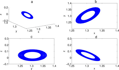
The phase diagram of system (2.2) with a = 1.5, b = 1.7, m = 0.02 and c = 0.05.

(5) When the parameter m ∈ [0.03,0.27], the controlled system keeps a cycle motion. The cycle gets lower as the parameter m increases, and the maximum Lyapunov exponents are always kept negative and get smaller, which implies that the controlled system tends to converge to a sink.

From the above results, we can find that, within m ∈ [−1.6,0.27], controlled system (2.2) has chaotic attractor, period montion and periodic windows. The behaviors of the system (2.2) become complex with varying m [22].

4 Hopf bifurcation analysis

In this part we discuss the Hopf bifurcation for the controlled system (2.2), applying normal form theory and Mathemaitca software.

Theorem 4.1

Suppose thata>0,b>0. While c goes through the critical valuec=c0=2bmba(a+m), system (2.2) plays a Hopf bifurcation at the equilibriumE+(b,b,cb).

Proof

Suppose that there is a pair of pure imaginary roots λ = ±iω(ω ∈ ℝ⁺) in characteristic equation.

We obtained

Δ(λ)=(iω)3+(m+a)(iω)2+(2b−acb)iω+2ab=0.

Hence one can see that

ReΔ(λ)=2ab−(a+m)ω2=0,ImΔ(λ)=i(−ω3+(2b−acb)ω)=0.

Thus we have

ω2=2aba+m,ω2=2b−acb.

Then

2aba+m=2b−acb.

By computing the equation, we get

2b>acb,c0=2bmba(a+m).

When c = c₀, one obtains

λ1=iω,λ2=−iω,λ3=−a−m,

where ω=2aba+m. Thus, when m > 0, c = c₀, the first condition of the Hopf bifurcation is satisfied.

From m > 0, it follows that

0=3λ2λ′+2(a+m)λλ′+(2b−acb)λ′−abλ,

λ′=aλ[3λ2+2(a+m)λ+2b]b−ac,

which indicates that

Re(λ′(c0))|λ=iω=−a(a+m)2b2b(a+m)3+4ab4≠0.

Thus, the proof of Theorem 4.1 is completed [27].

Remark 4.2

There is no Hopf bifurcation at the equilibriumE+(b,b,cb)while2b<acb.

Next, the expression, stability and size of bifurcating period solution in system (2.2) are studied, by using the normal form theory [27] and many rigid symbolic computation.

Theorem 4.3

If a > 0, b > 0, for the controlled system (2.2), bifurcating periodic solutions exist for sufficient small |c−c0|>0(c0=2bmba(a+m)). Furthermore, periodic solutions from Hopf bifurcation at E+(b,b,cb) have the following properties:

if M > 0, bifurcating periodic solutions of system (2.2) at E+(b,b,cb) are non-degenerate, supercritical and unstable;
if M < 0, bifurcating periodic solutions of system (2.2) at E+(b,b,cb) are non-degenerate, subcritical and stable;
the characteristic exponent and period of the bifurcating periodic solution are
β=β2ε2+O(ε4),T=2πω0(1+τ2ε2+O(ε4)),
whereω0=2aba+m,ε2=c−c0μ2+O[(c−c0)2]and
μ2=−ReC1(0)α′(0)=M−a(a+m)2b4ab4+2b(a+m)3,τ2=−μ2ω′(0)+ImC1(0)ω0=μ2ab2a(a+m)2ab2(a+m)3+4a2b5−N(a+m)2ab(a+m),β2=2ReC1(0)=2M,
whereM=Q2Q5+Q1Q6+12Im(g21)−22aba+m,N=Q1Q5−Q2Q6−2(Q12+Q22)−13(Q32+Q42)+12Re(g21)22aba+m,Re(g21)=(A13+B23)w11+12Re(w20)(A13−B23)−12Im(w20)(B13+A23),Im(g21)=(B13−A23)w11+12Im(w20)(A13−B23)−12Re(w20)(B13+A23),Re(w20)=(C11−C22)(a+m)−2C122aba+m(a+m)2−8aba+m,Im(w20)=(C11−C22)2aba+m−(a+m)C12(a+m)2−8aba+m,w11=C11+C22−2(a+m).
Q_i (i = 1,2,3, ⋯ , 6), and A₁₃, A₂₃, B₁₃, B₂₃, B₁₃,, are defined in Appendix.
(iv) the mathematical expression of Hopf bifurcation periodic solution of system (2.2) is
xyz=bbcb+cos⁡2πTtsin⁡2πTt0ε+γ1γ2(C11+C22)(1+Re(w20)cos⁡2πTt−Im(w20)sin⁡2πTt)−2(a+m)ε2+O(ε3),whereγ1=sin⁡4πTt(Q3+3Q5)−cos⁡4πTt(Q4−3Q6)−6Q262aba+m,γ2=Q3cos⁡4πTt−3Q5cos⁡4πTt+6Q1−Q4sin⁡4πTt−3Q6sin⁡4πTt62aba+m
Q_i (i = 1,2,3, ⋯ ,6) are defined in Appendix.

Proof

According to Theorem 4.1, while the parameter c changes and passes through the critical value c₀, Hopf bifurcation occurs at the equilibrium point E⁺, and its direction and stability are discussed below.

Because equilibrium E+(b,b,cb) is not in the origin, in order to shift it to the origin, let x = b√ + x₁, y = b√ + y₁ and z=cb+z1. Then, system (2.2) becomes

x1˙=a(y1−x1)y1˙=x1z1+cbx1+bz1+m(x1−y1)z1˙=−y12−2by1.

Denoting c=c0=2bmba(a+m), and linearizing system (2.2) at E+(b,b,cb) now yields the Jacobian matrix

J=−aa0m+cb−mb0−2b0,

and according to the matrix calculated above, we can get its characteristic equation:

Δ(λ)=λ3+(m+a)λ2+(2b−acb)λ+2ab=0.

By exact computations, we obtain λ₁ = ωi, λ₂ = −ωi and λ₃ = −a − m, when ω=2aba+m, and the corresponding eigenvectors respectively are

v1=−a2b(a+m)−a(a2+am)i−a(a2+2b+am)i(a2+2b+am)2(a+m),v2=−2ab(a+m)−2a(a2+am)i−a(a2+2b+am)i12(a2+2b+am)a+mandv3=−a(a+m)m(a+m)2mb.

For system (2.2), define

P~1=(Rev1,−Imv1,v3)=−a2b(a+m)a(a2+am)−a(a+m)0a(a2+2b+am)m(a+m)(a2+2b+am)2(a+m)02mb(3.1)

and make a transformation as follows:

(x1,y1,z1)T=P~1(x2,y2,z2)T.

Thus,

x˙2=−2aba+my2+F1(x2,y2,z2)y˙2=2aba+mx2+F2(x2,y2,z2)z˙2=−(a+m)z2+F3(x2,y2,z2)

where

F1(x2,y2,z2)=(A11x22+A12x2y2+A22y22+A13x2z2+A23y2z2+A33z22),F2(x2,y2,z2)=(B11x22+B12x2y2+B22y22+B13x2z2+B23y2z2+B33z22),F3(x2,y2,z2)=(C11x22+C12x2y2+C22y22+C13x2z2+C23y2z2+C33z22).

Furthermore, the following marks are consistent with [\cite{x}].

g11=14∂2F1∂x22+∂2F1∂y22+i∂2F2∂x22+∂2F2∂y22=12[(A11+A22)+i(B11+B22)],g02=i2∂2F1∂x2∂y2+∂2F2∂x22−∂2F2∂y22+14∂2F1∂x22−2∂2F2∂x2∂y2−∂2F1∂y22=12[i(A12+B11−B22)+(A11−B12−A22)],g20=14i∂2F2∂x22−∂2F2∂y22−2∂2F1∂x2∂y2+∂2F1∂x22+2∂2F2∂x2∂y2−∂2F1∂y22=12[i(B11−B22−A12)+(A11+B12−A22)],G21=18∂3F1∂x23+∂3F1∂x2∂y22+∂3F2∂x22∂y2+∂3F2∂y23+i∂3F2∂x2∂y22−∂3F2∂y23−∂3F1∂x22∂y2+∂3F2∂x23=0.

Meanwhile, one has

h111=14∂2F3∂x22+∂2F3∂y22=12(C11+C22),h201=14∂2F3∂x22−∂2F3∂y22−2i∂2F3∂x2∂y2=12(C11−C22−C12i).

Solving the following formula:

Dw11=−h111andw20(D−2iω0I)=−h201,

where D = −(a + m), one obtains

w11=C11+C22−2(a+m),w20=C11−C22−C12i−2(a+m)−4i2aba+m=Re(w20)+iIm(w20).

Where,

Re(w20)=(C11−C22)(a+m)−2C122aba+m(a+m)2−8aba+m,Im(w20)=(C11−C22)2aba+m−(a+m)C12(a+m)2−8aba+m.

Furthermore,

G1101=12i∂2F2∂x2∂z2−∂2F1∂y2∂z2+∂2F2∂y2∂z2+∂2F1∂x2∂z2=12[i(B13−A23)+B23+A13],G1011=12i∂2F2∂x2∂z2+∂2F2∂y2∂z2+∂2F1∂x2∂z2−∂2F2∂y2∂z2=12[i(B13+A23)+A13−B23],g21=G21+(2G1101ω11+G1011ω20)=Re(g21)+iIm(g21),

where

Re(g21)=(A13+B23)w11+12Re(w20)(A13−B23)−12Im(w20)(B13+A23),Im(g21)=(B13−A23)w11+12Im(w20)(A13−B23)−12Re(w20)(B13+A23).

Considering the above operation results, one can calculate the following formulas and get:

C1(0)=12g21+i2ω0−2g112+g11g20−13g022=M+Ni,μ2=−ReC1(0)α′(0)=−MRe(λ′(c0)),τ2=−μ2ω′(0)+ImC1(0)ω0=−μ2Im(λ′(c0)))+Nω0,β2=2ReC1(0)=2M,

where

ω0=2aba+m,α′(0)=Re(λ′(c0))=−a(a+m)2b2b(a+m)3+4ab4,ω′(0)=−a2a(a+m)2(a+m)3+4ab3.M=Q2Q5+Q1Q6+12Im(g21)−22aba+m,N=Q1Q5−Q2Q6−2(Q12+Q22)−13(Q32+Q42)+12Re(g21)22aba+m.

From a > 0, b > 0, one gets that α′(0) < 0, ω′(0) < 0 holds, so there are μ₂ > 0 and β₂ > 0with M > 0, which means that the Hopf bifurcation of system (2.2) at E₊(b√, b√,_cb√) is supercritical and non-degenerate, and the system's bifurcating periodic solution occurs and is unstable; if M < 0, then μ₂ < 0 and β₂ < 0, which means that the Hopf bifurcation of system (2.2) at E+(b,b,cb) is subcritical and non-degenerate, and the system’s bifurcating periodic solution occurs and is stable.

Moreover, the characteristic exponent and period are

β=β2ε2+O(ε4),T=2πω0(1+τ2ε2+O(ε4)),

where ε2=c−c0μ2+O[(c−c0)2].. The Hopf bifurcation periodic solution is

X(x1,y1,z1)T=P~1(x2,y2,z2)T=P~1Y,

while P˜₁ is a matrix and is described in (3.1),

x2=Reu,y2=Imu,z2=Re(ω20u2)+u2ω11+O(u3),

and

u=e2itπTε+ε2i6ω0[6g11+g02e−4itπT−3g20e4itπT]+O(ε3).

By complicate computations, one gets

xyz=bbcb+cos⁡2πTtsin⁡2πTt0ε+γ1γ2(C11+C22)(1+Re(w20)cos⁡2πTt−Im(w20)sin⁡2πTt)−2(a+m)ε2+O(ε3),

where γ₁, γ₂ are defined at Theorem 4.3.

Remark 4.4

The property of Hopf bifurcation at equilibriumE⁻can be considered in the same way.

Fix a = 5, b = 1.7, m = − 1 and the critical value c=c0=2bmba(a+m)≈−0.222. From the above theorems, near the equilibrium point E⁺, there are bifurcation periodic solutions for the controlled system (2.2) while c > c₀; E⁺ is stable while c < c₀, just as demonstrated in Fig.7.

$Fig. 7 (a) The phase diagram of system (2.2) with a = 5, b = 1.7, m = –1 and c = –0.22. (b) The phase diagram of system (2.2) with a = 5, b = 1.7, m = –1 and c = –0.32.$

Fig. 7

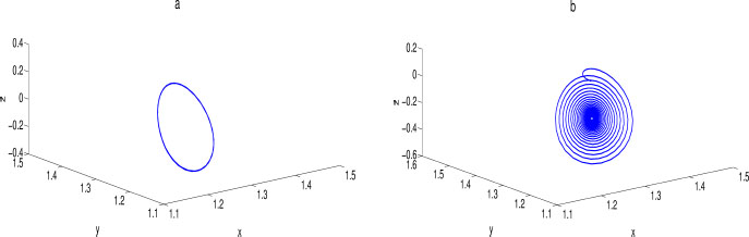
(a) The phase diagram of system (2.2) with a = 5, b = 1.7, m = –1 and c = –0.22. (b) The phase diagram of system (2.2) with a = 5, b = 1.7, m = –1 and c = –0.32.

5 Conclusions

In this paper the chaos and bifurcation are explored for the controlled chaotic system, which is put forward based on the hybrid strategy in an unusual chaotic system. Behaviors of the controlled system are studied through analyzing its corresponding bifurcation diagrams and Lyapunov exponents, showing that there exist chaotic area, period area and several periodic windows within the range of variable parameter. The results show that the controlled system maintains the local structure and dimension of the original system, and the dynamics behavior of the controlled system is much richer than the original system. Furthermore, a sufficient condition for the existence of Hopf bifurcation of the controlled chaotic system is obtained. Using the normal form theory, the direction and stability of bifurcating periodic solution are verified. Numerical simulations demonstrate the theoretical analysis results.

Appendix

For convenience, some values of the symbols used in Theorem 4.3 are given in this section.

D~=−2bm+(a+m)(2b+(a+m)2),D1=[2b+a(a+m)]2(a+m)D~:D2=(a2+2b+am)a(a+m)D~,D3=a+mD~,A11=4abma+m2D~,A12=−2amab[2b(a+m)+a(a−m)2]2b+a(a+m)D~,A22=−a[2b+a(a+m)][2b+(a+m)2]2(a+m)D~,A13=2amb[a(a+m)2+2b(a+m)][2b+a(a+m)]D~,A23=−2ma(a+m)[(a+m)(4ab+a(a+m)2)+2b(b+m2)]2[2b+a(a+m)]D~,A33=−m2a+m[(a+m)3−2b(a−m)]2[2b+a(a+m)]D~,B11=−2a2b(a+m)[2b+(a+m)2]aD~:B12=2a2(s+m)(2b(a+m)2)D~,B22=−amb(a+m)(2b+a(a+m))aD~,B13=−2a2[(a+m)2+2b][a(a+m)2+am2+2b(a+m)]a(a2+2b+am)D~,B23=2mab(a+m)[a2(a2+2b+am)−m(a+m)(2b−am)]a(a2+2b+am)D~,B33=−mb(a+m)[(a+m)2(2a2+m2)+4a2b]a(a2+2b+am)D~,C11=−2ab(2b+a(a+m))(a+m)2D~,C12=a(a+m)22a(a+m)[(2b+a(a+m)]D~,C22=ab[2b+a(a+m)]2D~,C13=−a2(a+m)[(a+m)2(a+2b+am)+2bm(a+m)]D~,C23=4m(a+m)ab[b+a(a+m)]D~,C33=mb(a+m)2(m−2a)D~,Q1=12(A11+A22),Q2=12(B11+B22),Q3=12(A11−B12−A22),Q4=12(B11+A12−B22),Q5=12(A11+B12−A22),Q6=12(B11−A12−B22).

Acknowledgement

The authors wish to thank the reviewers for their constructive and pertinent suggestions for improving the presentation of the work. This work was supported by the National Natural Science Foundation of China (Grant No. 11561069), the Guangxi Natural Science Foundation of China (Grant Nos. 2016GXNSFBA380170, 2017GXNSFAA198234) and the Guangxi University High Level Innovation Team and Distinguished Scholars Program of China (Document No. [2018] 35).

References

[1] Lorenz E.N., Deterministic nonperiodic flow. Journal of Atmospheric Sciences, 1963, 20, 130-141.10.1175/1520-0469(1963)020<0130:DNF>2.0.CO;2Search in Google Scholar

[2] Chen G., Ueta T., Yet another chaotic attractor. International Journal of Bifurcation and Chaos, 1999, 9, 1465-1466.10.1142/S0218127499001024Search in Google Scholar

[3] Lü J., Chen G., A new chaotic attractor coined. International Journal of Bifurcation and Chaos, 2002, 12, 659-661.10.1142/S0218127402004620Search in Google Scholar

[4] Vaněč A., Čelikovský S., Control systems: from linear analysis to synthesis of chaos. Prentice Hall International (UK) Ltd, 1996, 4, 1479-1480.Search in Google Scholar

[5] Sprott J.C., Some simple chaotic flows, Physical review E, 1994, 50, R647-R650.10.1103/PhysRevE.50.R647Search in Google Scholar

[6] Rösler O.E., An equation for continuous chaos. Physics Letters A, 1976, 57, 397-398.10.1016/0375-9601(76)90101-8Search in Google Scholar

[7] Chua L.O., Matsumoto T., Komuro M., The double scroll family. IEEE Transactions on Circuits and Systems I-Fundamental Theory and Applications, 1985, 32, 798-818.10.1109/TCS.1985.1085791Search in Google Scholar

[8] Qi G., Chen G., Du S., et al., Analysis of a new chaotic system. Physica A Statistical Mechanics and Its Applications, 2005, 352, 295-308.10.1016/j.physa.2004.12.040Search in Google Scholar

[9] Sundarapandian V., Pehlivan I., Analysis, control, synchronization, and circuit design of a novel chaotic system. Mathematical and Computer Modelling, 2012, 55, 1904-1915.10.1016/j.mcm.2011.11.048Search in Google Scholar

[10] Pehlivan I., Uyaroglu Y., A new 3D chaotic system with golden proportion equilibria: Analysis and electronic circuit realization. Computers and Electrical Engineering, 2012, 38, 1777-1784.10.1016/j.compeleceng.2012.08.007Search in Google Scholar

[11] Wei Z., Moroz I., Wang Z., Zhang W., Detecting hidden chaotic regions and complex dynamics in the self-exciting homopolar disc dynamo. International Journal of Bifurcation and Chaos, 2017, 27, 1730008.10.1142/S0218127417300087Search in Google Scholar

[12] Čelikovský S., Chen G., On a generalized Lorenz canonical form of chaotic systems. International Journal of Bifurcation and Chaos, 2002, 12, 1789-1812.10.1142/S0218127402005467Search in Google Scholar

[13] Yang Q., Chen G., A chaotic system with one saddle and two stable node-foci. International Journal of Bifurcation and Chaos, 2008, 18, 1393-1414.10.1142/S0218127408021063Search in Google Scholar

[14] Yang Q., Wei Z., Chen G., An unusual 3D autonomous quadratic chaotic system with two stable node-foci. International Journal of Bifurcation and Chaos, 2010, 20, 1061-1083.10.1142/S0218127410026320Search in Google Scholar

[15] Wei Z., Yang Q., Dynamical analysis of a new autonomous 3-D chaotic system only with stable equilibria. Nonlinear Analysis: Real World Applications, 2011, 12, 106-118.10.1016/j.nonrwa.2010.05.038Search in Google Scholar

[16] Cai P., Tang J., Li Z., Controlling Hopf bifurcation of a new modified hyperchaotic L system. Mathematical Problems in Engineering, 2015.10.1155/2015/614135Search in Google Scholar

[17] Cai P., Tang J., Li Z., Analysis and controlling of Hopf bifurcation for chaotic van der Pol-Duffing system. Mathematical and Computational Applications, 2014, 19, 184-193.10.3390/mca19030184Search in Google Scholar

[18] Ding D., Zhang X., Cao J., et al., Bifurcation control of complex networks model via PD controller. Neurocomputing, 2016, 175, 1-9.10.1016/j.neucom.2015.09.094Search in Google Scholar

[19] Cheng Z., Li D., Cao J., Stability and Hopf bifurcation of a three-layer neural network model with delays. Neurocomputing, 2016, 175, 355-370.10.1016/j.neucom.2015.10.068Search in Google Scholar

[20] Wei Z., Moroz I., Wang Z., Sprott J.C., Kapitaniak T., Dynamics at infinity, degenerate Hopf and zero-Hopf bifurcation for Kingni-Jafari system with hidden attractors. International Journal of Bifurcation and Chaos, 2016, 26, 1650125.10.1142/S021812741650125XSearch in Google Scholar

[21] Li J., Liu Y., Wei Z., Zero-hopf bifurcation and Hopf bifurcation for smooth Chua's System. Advances in Difference Equations, 2018, 141.10.1186/s13662-018-1597-8Search in Google Scholar

[22] Liu Y., Pang S., Chen D., An unusual chaotic system and its control. Mathematical and Computer Modelling, 2013, 57, 2473-2493.10.1016/j.mcm.2012.12.006Search in Google Scholar

[23] Geng F., Li X., Singular orbits and dynamics at infinity of a conjugate Lorenz-like system. Mathematical Modelling and Analysis, 2015, 20, 148-167.10.3846/13926292.2015.1019944Search in Google Scholar

[24] Wang H., Li X., New results to a three-dimensional chaotic system with two different kinds of nonisolated equilibria. Journal of Computational and Nonlinear Dynamics, 2015, 10, 161-169.10.1115/1.4030028Search in Google Scholar

[25] Wei Z., Pham V.T., Kapitaniak T., Wang Z., Bifurcation analysis and circuit realization for multiple-delayed Wang-Chen system with hidden chaotic attractors. Nonlinear Dynamics, 2016, 85, 1635-1650.10.1007/s11071-016-2783-4Search in Google Scholar

[26] Guckenheimer J., Holmes P., Nonlinear oscillations, dynamical systems, and bifurcations of vector fields . Physics Today, 1985, 38, 102-105.10.1063/1.2814774Search in Google Scholar

[27] Hassard B.D., Kazarinoff N.D., Wan Y.H., Theory and applications of Hopf bifurcation. Cambridge Univ., London, 1981.Search in Google Scholar

[28] Neuts M.F., Matrix-geometric solutions in stochastic models: an algorithmic approach. Johns Hopkins University Press, 1981.Search in Google Scholar

Received: 2018-08-03

Accepted: 2018-09-14

Published Online: 2018-11-03

This work is licensed under the Creative Commons Attribution-NonCommercial-NoDerivatives 4.0 License.

Articles in the same Issue

https://doi.org/10.1515/math-2018-0105

Keywords for this article

Controlled chaotic system; Chaos; Bifurcation; Normal form theory

Creative Commons

BY-NC-ND 4.0