Endpoint prediction of BOF steelmaking based on state-of-the-art machine learning and deep learning algorithms

3.1 Time series data

A time series consists of a sequence of random variables arranged chronologically. In a two-dimensional context, it typically represents the curves of the target process, sampling values at a specified rate, and with uniform time intervals. The time series data for TSO prediction consists of seven curves, which are curves of off-gas total flow (Gas-Flow), lance height (Lc-Height), cumulative oxygen consumption (O₂-Blow), and gas percentage of carbon monoxide (GP-CO), carbon dioxide (GP-CO₂), oxygen (GP-O₂), and hydrogen (GP-H₂). Off-gas refers to the reaction gas produced during BOF steelmaking. The off-gas profile refers to the collective term for percentage amount curves of four gases, which sensitively reflect the steelmaking reactions. Depending on the sampling sequence of the BOF system, the time interval between each time step is 1 s. As the steelmaking time varies for each heat, all the time series were zero-padded to 1,024 time-steps. An example of an original time series is illustrated in Figure 1.

Figure 1

An example of an un-padded time series. (a) Off-gas profile; (b) curves of oxygen lance height, accumulative oxygen consumption, and off-gas flow rate.

3.2 Tabular data

The columns in tabular data define the features (tabular features), while the rows represent the values of each heat for these features. Table 1 displays the features of tabular data and their distribution. It consists of features of endpoint targets, information of hot metal, scraps, additives, blowing practices, and Temperature, Sample, Carbon test (TSC) related features. The pre-set oxygen blown values came from second calculation.

3.3 Mixed data

Mixed data contained both tabular and time series data.

3.4 Targets and error metrics

The targets are molten steel’s contents of phosphorus (Endpoint [P] (%)), carbon (Endpoint [C] (%)), and temperature (Endpoint-Temp (°C)) in endpoint. The target values in dataset are measured from TSO test. The distributions and relationships of the targets are shown in Figure 2.

Figure 2

The statistical distributions and relationships of the targets.

Combinatorial metrics were used to evaluate the model. The basic metrics adopted were MSE = 1 n ∑ i = 1 n ( Y i − Y ˆ ) 2 and MAE = 1 n ∑ i = 1 n | Y i − Y ˆ | , where MSE is the mean square error; MAE is the mean absolute error; ; Y i is the true value of target with index i in dataset X ; Y ˆ is the predicted value of Y i ; and n is the number of samples contained in X . Traditional methods of assessing hit rates based on uniform standards are not applicable due to significant differences in the end points of various steel grades. In this study, the determination of the hit range is based on the target value. In on-site production, a statistical hit rate of ± 10 , ± 15 , and ± 20 % around the target value is commonly applied for chemical tests. For temperature, this ranges are ± 10 , ± 15 , and ± 20 ℃ . SO, following metrics were also used to assist the evaluation:

1. The proportion of the predicted value distributes within ± 10 , ± 15 , and ± 20 % of the true value of Endpoint [P] and Endpoint [C].

2. The proportion of the predicted value of Endpoint-Temp distributes within ± 10 , ± 15 , and ± 20 ℃ of the true value.

3.5 Hyper-parameters tuning

The models were auto tuned with Bayesian optimization for 2,000 trials. Then, manual tuning is used to further adjust the hyper-parameters. The hyper-parameter boundaries and optimum hyper-parameters for ML models and the best models are detailed in the appendix.

4.1 ML with tabular data

The subsequent ML models are employed for predicting endpoint values using tabular data. It is a data mining process, and the inputs are tabular data.

XGBoost [23]. XGBoost is an ML algorithm rooted in the gradient boosting framework, employing CART decision trees as its base learner. It enhances performance by integrating second-order Taylor series expansion and regularization into the loss function, optimizing it using the Newton-Raphson method rather than gradient descent. Furthermore, it implements techniques such as shrinkage, column subsampling, handling missing values, and feature block arrangement to improve predictive accuracy. Its structure is shown in Figure 3. It has the advantages of regularization that helps simplify models and prevent overfitting. However, it suffers from an abundance of algorithm parameters and is not suitable for handling ultra-high-dimensional feature data.

Figure 3

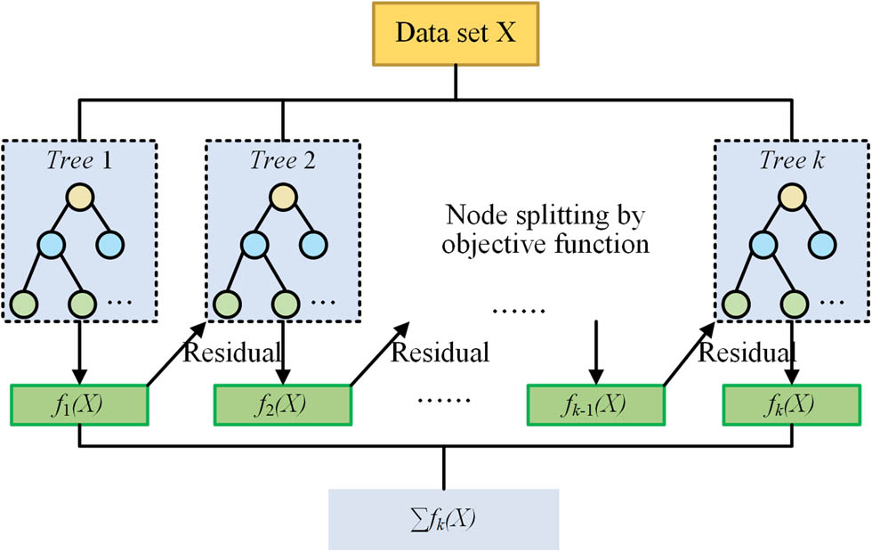
Structure of XGBoost, f K is loss function in k th tree.

LightGBM [24]. LightGBM is an ML algorithm rooted in the gradient boosting framework. It introduces innovation through the histogram algorithm, which discretizes continuous float eigenvalues into k integers and constructs a histogram with a width of k . This histogram accumulates necessary statistics after traversing the dataset. Subsequently, an optimal segmentation point is determined based on the discrete values of the histogram. LightGBM employs a leaf-wise strategy for splitting, prioritizing leaves with the highest split gain, thereby achieving superior precision compared to the level-wise approach. It has the advantages of low memory occupation and higher accuracy, but it uses deeper trees that are easier to overfit. Its structure is shown in Figure 4.

Figure 4

Structure of LightGBM.

CatBoost [25]. CatBoost is an ML algorithm built upon the gradient boosting framework, utilizing oblivious trees as its base learner. It incorporates techniques such as null value processing, ordered target statistics encoding, and feature combinations to handle categorical features effectively. To address prediction shift issues, CatBoost employs an ordered boosting algorithm. Notably, it conducts categorical feature processing during training rather than as a pre-processing step. During the training process, CatBoost computes both random combinations of target statistics σ cat and random combinations of ordered boosting σ boost . It has high accuracy and low requirements for data pre-processing but need more memory storage. Its structure is shown in Figure 5.

Figure 5

Structure of CatBoost, N is number of samples.

TabNet [26]. TabNet is a neural network-based ML algorithm that employs the sequential attention mechanism to mimic decision tree algorithms. Sequential attention consists of two crucial steps: utilizing the Attentive Transformer to identify important features and employing the Feature Transformer to convert feature values into a feature map. Both the Attentive Transformer and Feature Transformer utilize a feature block composed of a fully connected layer, batch normalization layer, and gated linear unit activation function in sequence as their base learner. Sparse regularization is utilized as the loss function. It is more suitable for fine-tuning and transfer learning, but it is prone to overfitting. Its structure is shown in Figure 6.

Figure 6

Structure of TabNet: (a) Tabnet encoder structure, Agg. is aggregate process, (b) Tabnet decoder structure, (c) feature transformer structure, and (d) attentive transformer structure.

Importance analysis. Aside from data mining, further analysis of feature importance in tabular data is conducted based on the average scaled importance values assigned to each feature by all models above. This analysis combines these importance values with the slope sign derived from linear regression results. The culmination of this analysis is presented in Section 5.

4.2 Time series analysis models with time series data

After padding and channel-wise standardization, the time series is input into the following models to predict TSO values. The input time series has dimensions of 7 channels and 1,024 time-steps. The following are SOTA models for different time series classification and prediction tasks (these two tasks are collectively referred to as time series analysis). They efficiently extract features from time series data and make accurate predictions. Their outputs are flattened and project to single values. The following is a brief overview of each model.

1D ResCNN (ResCNN) [27]. ResCNN is a convolutional neural network (CNN) using residual connections. To enhance the robustness of the model, residual block was fixed to the first three convolutional layers and different activation functions were adopted in different layers. In case of overfitting, global average pooling is applied instead of fully connected layer.

TCN [28]. TCN is a model based on one-dimensional (1D) CNN. Its main characteristics are causal convolution, dilation convolution, and residual connection. Causal convolution ensures that the output of each time step is only related to previous time step. And dilation convolution enhances the limited receptive field of causal convolution.

OmniScaleCNN (OS-CNN) [29]. OS-CNN is a model based on 1D CNN. Omni-Scale Block was proposed to increase 1D CNN receptive field and improve model robustness. This block automatically adjusts the kernel size and receptive field according to different time series to get the highest accuracy.

XCM [30]. XCM is a compact model based on 1D CNN. It accurately identifies and utilizes important time steps by Gradient-weighted Class Activation Mapping, which is a post hoc model-specific explainability method.

TST [31]. TST is based on self-attention mechanism. Its base learner is self-attention layer that consists of multi-head attention network, feedforward network, and residual connection. The TST framework introduces an unsupervised pre-training regimen to provide significant performance benefits.

LSTM-FCN [32]. LSTM-FCN uses both LSTM module and FCN module. The time series sensitivity is enhanced by adding LSTM modules. In particular, there are 1D CNN layers with batch normalization and layers with shuffle and dropout. The output of FCN and LSTM is concatenate as the final output.

D-linear [33]. The main feature extraction mechanism of the D-linear model is a linear layer network. It decomposes historical time series data into trend and remainder components with linear layer networks. Positional encoding is introduced during the decomposition to preserve sorting information. In this study, D-Linear-I was utilized to address underfitting resulting from weight sharing between different features, ensuring each feature has its independent linear layer.

The structures of time series analysis models are shown in Figure 7

Figure 7

The structure of all the time series analysis models. The outputs of all models are flattened and processed by a fully connected layer with dropout to produce a single output, and training will be conducted using the rooted mean squared error (RMSE) loss function. And Conv1d is 1D convolutional network, Conv2d is two-dimensional convolutional network. k is the number of split token of inputs and latent. The structures are (a) 1D ResCNN; (b) TCN, B₁ is the number of shown block; (c) OS-CNN; (d) XCM; (e) TST, z , and u are processed token, and B₂ is the number of transformer encoder; (f) LSTM-FCN; and (g) D-linear.

Importance analysis of time series. After TSO prediction, for further studying the relationship between TSO values and time series data, a single-layer gated recurrent unit (GRU) network based on the attention mechanism was developed. The hidden of the last time step was taken as Query, the hidden of each time step was taken as Key and Value for dot product according to equation (1) [30]. By extracting the dot product results after Softmax operation, the weights (importance) of each time step can be obtained. With another single-layer attention based GRU with permuted time series, the weights of each channel can be also received.

4.3 Image analysis models with time series data

Each time series sequence tensor, consisting of 1,024 time-steps and 7 channels, was resized to a 32 × 32 image tensor with 7 channels to facilitate higher-dimensional feature extraction. This transformation converted endpoint prediction into an image regression task. SOTA image classification and regression (collectively referred to as image analysis) models were modified for image regression. The outputs of the models were flattened and projected to single values.

Pre-activation ResNet [34]. Pre-activation ResNet is founded upon CNNs, emphasizing direct transmission of feature information between modules. In its architecture, the conventional residual block is substituted with two sequentially arranged modules comprising batch normalization, ReLU functions, and convolutional layers. This substitution alleviates the training complexity of deep networks while preserving the model’s parameter capacity.

DenseNet [35]. DenseNet is a CNN architecture designed to address the issue of gradient vanishing. In the DenseNet structure, each layer’s input is derived from the outputs of all preceding layers, establishing direct connections from early layers to later ones. Batch normalization and ReLU activation functions are employed between each convolutional layer. This design promotes information flow throughout the network, facilitating efficient gradient propagation and enhancing training performance.

Deep layer aggregation (DLA) [36]. DLA serves as a foundational structure for consolidating deep networks. It encompasses two distinct types of aggregations: Iterative deep aggregation (IDA) and Hierarchical deep aggregation (HDA). In IDA, the aggregation node’s input comprises the output of the current stage and the previous node. Conversely, in HDA, the aggregation node’s input consists of the outputs of blocks and the preceding node, while the aggregation node’s output is also fed into the subsequent set of blocks. In this study, DLA, based on two-dimensional convolutional networks, utilizes IDA to amalgamate stages and HDA to consolidate blocks within each stage.

Dual path networks (DPN) [37]. DPN is a model that integrates key features from ResNet and DenseNet architectures. The practical implementation of the DPN network adopts ResNeXt, leveraging group convolution instead of ResNet, as the primary component. This modification effectively enhances the learning capacity of each block while mitigating the rapid expansion of DenseNet channels. Subsequently, slice and concatenate layers are applied to introduce additional DenseNet pathways. Notably, split and elementwise addition operations are performed on the outputs of both model components.

GoogleNet (Inception-ResNet v2) [38]. GoogleNet, founded on CNNs, introduces the inception module, aimed at reducing model parameters and enhancing network complexity. Inception-ResNet v2, an advancement over GoogleNet, incorporates residual connections to enable a deeper model structure. Key components include inception modules such as the Inception-ResNet-A block, utilizing 1 × 1 and 3 × 3 convolutions with residual connections, the Inception-ResNet-B block employing 1 × 1, 1 × n, and n × 1 convolutions with residual connections, and the Inception-ResNet-C block integrating 1 × 1, 1 × 3, and 3 × 1 convolutions with residual connections. In comparison to Inception V4, it offers greater ease of tuning.

Vision transformer (VIT) [39]. Vision transformer is rooted in the transformer architecture. It introduces a multi-head attention mechanism utilizing dot product, where each transformer layer comprises layer normalization, a feedforward network, and multi-head attention sequentially, with residual connections. VIT begins by embedding and projecting a patched image (C × H × W) to resize it to C × D. Following patch embedding and position embedding, the transformed image is forwarded to the transformer encoder to produce the final output.

The schematic diagram of the image regression process and the structures of SOTA backbones used are depicted in Figure 8.

Figure 8

Diagram of the image regression process and the structures of SOTA backbones. (a) Diagram of the image regression process. The structures are (b) Pre-activation ResNet; (c) DenseNet; (d) DLA; (e) DPN; (f) GoogleNet; and (g) VIT.

4.4 Concat-model and paral-model with mixed data

To further explore methods for optimizing the utilization of available data and enhancing prediction accuracy, two DL architectures were designed for making prediction with both tabular and time series data. Their architectures are shown in Figure 9.

Figure 9

Architectures of (a) Concat-model and (b) paral-model, FC is fully connected layer. For keeping the same complexity, the tabular data are embedded in the same pattern.

The first architecture is named concat-model. It involves embedded and reshaped tabular data, then concatenating it with the time series data in the channel dimension to form a new sequence. This new sequence will be input into time series analysis models for prediction.

The second architecture is dubbed the paral-model. It employs time series analysis models to handle time series data, while simultaneously utilizing a tabular data processing network composed of fully connected layers with dropout to process tabular data. The outputs of these two networks are added, flattened, and projected as the final output.

5.1 Results of tabular feature importance

Figure 10 shows the tabular features and their feature importance in different tasks. And Figure 10 shows the distribution of importance across channels and time steps for the time series data in different prediction tasks. The features related to hot metal and oxygen blowing are more important in each task. The features related to additives are of lower importance.

Figure 10

Importance analysis result for different task.

Time series data from 300 heats were randomly chosen for channel and time step importance analysis. Figure 11 is importance analysis results of time series data. It demonstrates that time series data exhibit comparable distributions of time step and channel importance for predicting Endpoint [P] and Endpoint [C]. Later stage time steps and channels of O₂-blow, flow, and CO are more crucial for predicting Endpoint [P]/[C]. However, for Endpoint-Temp, mid-stage time steps are more important, while channels of GP-CO, GP-CO₂, and GP-O₂ exhibit lower importance for prediction. For each target, the blowing practice related curves are more important.

Figure 11

Importance analysis results of time series data’s time steps and channels in different task.

5.2 Results of ML with tabular data

The prediction results of test set are shown in Table 2. Conventional BP-NN and SVR are also considered, and their performance are also listed and compared. The best values are given in bold.

Table 2 indicates that the targets exhibit high predictability with tabular data. Across the same task, the discrepancy in accuracy among models was minimal. Additionally, most predicted values fell within ± 20% or ± 20°C of actual values for Endpoint [P]/[C]/Temp prediction. Based on MAE, CatBoost emerges as the optimal model for Endpoint [P] and Endpoint [C] prediction, while LightGBM excels in Endpoint-Temp prediction. The conventional BP-NN performed worse in each task. However, it is worth noting that CatBoost and TabNet have extremely slower training processes with low learning rates.

5.3 Results of time series analysis models with time series data

The performance of time series analysis models with different SOTA backbones on the test set is presented in Table 3, and the models are named with the backbones’ name. The best values are given in bold. The training strategies are demonstrated in appendix section.

According to Table 3, approximately 70% of the predicted values for Endpoint [C] and Endpoint [P] fell within ± 20 % of the actual values. For Endpoint-Temp, nearly 90% of the predictions were within ± 20 ℃ of the true values. These results demonstrate a strong correlation between time series data and TSO values. It can be concluded that OS-CNN exhibited the highest accuracy for predicting Endpoint [P] and Endpoint-Temp, while ResCNN performed best for predicting Endpoint [C]. Compared to ML models, using only time series data yields lower accuracy for predicting Endpoint [P] and Endpoint-Temp but higher accuracy for predicting Endpoint [C].

5.4 Results of image analysis models with time series data

The performance of image analysis models utilizing different SOTA backbones is depicted in Table 4. Model names are the same as backbones’ name. The best values are given in bold. Table 4 indicates that image analysis models did not enhance forecasting accuracy. The best prediction effect of image analysis models with different backbone is similar to time series models. However, in practical scenarios, after hyperparameter tuning, image analysis models necessitate more parameters and are more prone to overfitting. Therefore, if only time series data are accessible for forecasting, time series DL models are recommended.

5.5 Results of concat-model and paral-model with mixed data

The prediction of concat-model and paral-model with different backbones is shown in Tables 5 and 6. They demonstrate that using mixed data with DL models can enhance the prediction accuracy of Endpoint [P]/[C]/Temp compared to using only time series data, especially for Endpoint-Temp. The concat-model outperforms the paral-model, achieving higher accuracy and reducing MAE by 4–10%. These findings suggest that a DL model using composite inputs may perform better than a DL model using only one of the inputs. At the same time, the way of feature merging also affects the prediction efficiency. The earlier the feature fusion is performed, the higher the feature fusion efficiency may be. Besides, the results also show that a single network can extract information from merged features efficiently. The best values are given in bold.

The visualized best prediction results in test set for each task is shown in Figure 12. The models are concat-model with backbone of TCN (for Endpoint [P]) and ResCNN (for Endpoint [C]/Endpoint-Temp).

Figure 12

Running chart of prediction results of best models.

According to all the above results, concat-models with TCN and ResCNN as backbone are the best models. A five-fold cross-validation is used to strengthen the reliability of the model evaluations and further optimize the hyperparameters. Specifically, the training set is mixed with the validation set and the order is randomly shuffled. For a set of model hyperparameters, 0–20, 20–40, 40–60, 60–80, and 80–100% of this new dataset are used for model validation, respectively, while the remaining data are used for training. The average of the results of these five training sessions is used for selecting the best hyper-parameters. The performance of the models with the best hyperparameters in the test set is shown in Table 7.

After five-fold cross-validation, the performance of the model was further improved. The adjustment of hyperparameters is also experienced by all the training set and test set data, so that the model has stronger confidence.

5.6 Results of comparison with other public works

The MAE and MSE of BOF endpoint prediction obtained from previous studies are juxtaposed with those derived from this work. Despite differences in data quality, objectives, application scenarios, BOF vessel structure, and steelmaking processes across these studies compared to the scenario addressed in this study, they still hold significance for reference and comparison purposes. The results are shown in Table 8.

6.1 Significance of predictions

1. Optimizing the steelmaking process. (1) The models allow for continuous output of predictions. In the later stages of smelting, since the additives have been completed, for the model, its predictions are solely related to the time series and the oxygen blowing volume is updated every second. With such dynamic inputs, the models can generate a decarburization/temperature rise curve to dynamically control the endpoint accordingly (The “Dynamic” mode of the prediction software). (2) The importance analysis based on the developed model has demonstrated the significance of various inputs, enabling targeted adjustments to the process based on their importance. For instance, in controlling the endpoint temperature, attention should be paid to controlling the amount of Newman ore added according to the steel grade and process requirements.

2. Reduce resource consumption. By eliminating the TSO test, each heat can directly save $20–30 in disposable sampler consumption. Along with savings in cooling and driving energy consumption, even if only 50% of heats cancel the TSO test, each steel plant can save nearly half million dollars annually.

3. Improve production efficiency. According to the predicted values, the TSO test can be eliminated. This directly saves 1.5–2 min of smelting time. With a BOF steelmaking time of 10–15 min, the efficiency is increased by 12–20%.

4. Additionally, this study has demonstrated that relatively accurate endpoint predictions can be achieved solely using time series data. Some factories have poor data infrastructure, with incomplete static figures or data that cannot be utilized due to manual input. In such cases, if there are oxygen blowing-related curves and gas composition data from coal gas recovery, endpoint prediction can still be achieved.

References

[1] Wang, Z., Q. Liu, F. M. Xie, B. Wang, B. Wang, X. C. Lu, et al. Model for prediction of oxygen required in BOF steelmaking. Ironmaking & Steelmaking, Vol. 39, No. 3, 2012, pp. 228–233.Suche in Google Scholar
[2] He, F. and L. Zhang. Prediction model of end-point phosphorus content in BOF steelmaking process based on PCA and BP neural network. Journal of Process Control, Vol. 66, 2018, pp. 51–58.Suche in Google Scholar
[3] Wang, Z., J. Chang, Q.-P. Ju, F.-M. Xie, B. Wang, H.-W. Li, et al. Prediction Model of End-point Manganese Content for BOF Steelmaking Process. ISIJ international, Vol. 52, No. 9, 2012, pp. 1585–1590.Suche in Google Scholar
[4] Li, W., Q. M. Wang, X. S. Wang, and H. Wang. Magnetically separable Ag/AgCl-zero valent iron particles modified zeolite X heterogeneous photocatalysts for tetracycline degradation under visible light. Chemical Engineering Transactions, Vol. 51, 2016, pp. 475–480.Suche in Google Scholar
[5] Wang, R., I. Mohanty, A. Srivastava, T. K. Roy, P. Gupta, and K. Chattopadhyay. Hybrid method for endpoint prediction in a basic oxygen furnace. Metals, Vol. 12, No. 5, 2022, id. 801.Suche in Google Scholar
[6] Kang, Y., M. M. Ren, J. X. Zhao, L. B Yang, Z. K. Zhang, Z. Wang, and G. Cao. Prediction of end-point phosphorus content of molten steel in BOF with machine learning models. Journal of Mining and Metallurgy, Section B: Metallurgy, 2024, 8–8.Suche in Google Scholar
[7] Zhou, K. X., W. H. Lin, J. K. Sun, J. S. Zhang, D. Z. Zhang, X. M. Feng, et al. Gasification reactivity and kinetic parameters of coal chars for non-isothermal steam gasification. J. Iron Steel Res. Int., Vol. 28, 2021, pp. 1–10.Suche in Google Scholar
[8] Bae, J., Y. Li, N. Ståhl, G. Mathiason, and N. Kojola. Using Machine Learning for Robust Target Prediction in a Basic Oxygen Furnace System. Metallurgical and Materials Transactions B, Vol. 51, 2020, pp. 1632–1645. (ANN, SVR).Suche in Google Scholar
[9] Cox, I. J., R. W. Lewis, R. S. Ransing, H. Laszczewski, and G. Berni. Application of neural computing in basic oxygen steelmaking. Journal of Materials Processing Technology, Vol. 120, No. 1, 2002, pp. 310–315.Suche in Google Scholar
[10] Liu, Z., S. Cheng, and P. P. Liu. Prediction model of BOF end-point P and O contents based on PCA–GA–BP neural network. High Temperature Materials and Processes, Vol. 41, No. 1, 2022, pp. 505–513.Suche in Google Scholar
[11] Gao, C., M. Shen, X. Liu, L. Wang, and M. Chen. In vitro digestion of bread: How is it influenced by the bolus characteristics? Transactions of the Indian Institute of Metals, Vol. 72, 2019, pp. 257–270.Suche in Google Scholar
[12] Schlueter, J., H. J. Odenthal, N. Uebber, H. Blom, and K. Morik. A novel data-driven prediction model for BOF endpoint. Proceedings of the Iron & Steel Technology Conference, 2013, pp. 923–928.Suche in Google Scholar
[13] Duan, J., Q. Qu, C. Gao, and X. Chen. BOF steelmaking endpoint prediction based on FWA-TSVR. In 2017, 36th Chinese Control Conference (CCC), IEEE, 2017, pp. 4507–4511.Suche in Google Scholar
[14] Shao, Y., M. Zhou, Y. Chen, Q. Zhao, and S. Zhao. BOF endpoint prediction based on the flame radiation by hybrid SVC and SVR modeling. Optik, Vol. 125, No. 11, 2014, pp. 2491–2496.Suche in Google Scholar
[15] Zhou, M., Q. Zhao, and Y. Chen. Endpoint prediction of BOF by flame spectrum and furnace mouth image based on fuzzy support vector machine. Optik, Vol. 178, 2019, pp. 575–581.Suche in Google Scholar
[16] Jiang, F., H. Liu, B. Wang, and X. F. Sun. Emotional Regulation and Executive Function Deficits in Unmedicated Chinese Children with Oppositional Defiant Disorder. Computer Engineering, Vol. 42, No. 10, 2016, pp. 277–282.Suche in Google Scholar
[17] Borisov, V., T. Leemann, K. Seßler, J. Haug, M. Pawelczyk, and G. Kasneci. Deep neural networks and tabular data: A survey. IEEE Transactions on Neural Networks and Learning Systems, 2022.Suche in Google Scholar
[18] Grinsztajn, L., E. Oyallon, and G. Varoquaux. Why do tree-based models still outperform deep learning on typical tabular data?. Advances in Neural Information Processing Systems, Vol. 35, 2022, pp. 507–520.Suche in Google Scholar
[19] Lim, B. and S. Zohren. Time-series forecasting with deep learning: a survey. Philosophical Transactions of the Royal Society A, Vol. 379, No. 2194, 2021, id. 20200209.Suche in Google Scholar
[20] Ismail Fawaz, H., G. Forestier, J. Weber, L. Idoumghar, and P. A. Muller. Accurate and interpretable evaluation of surgical skills from kinematic data using fully convolutional neural networks. Data Mining and Knowledge Discovery, Vol. 33, No. 4, 2019, pp. 917–963.Suche in Google Scholar
[21] Rawat, W. and Z. Wang. Deep convolutional neural networks for image classification: A comprehensive review. Neural Computation, Vol. 29, No. 9, 2017, pp. 2352–2449.Suche in Google Scholar
[22] Meer, P., D. Mintz, A. Rosenfeld, and D. Y. Kim. Robust regression methods for computer vision: A review. International Journal of Computer Vision, Vol. 6, 1991, pp. 59–70.Suche in Google Scholar
[23] Chen, T. and C. Guestrin. Xgboost: A scalable tree boosting system. In Proceedings of the 22nd ACM SIGKDD International Conference on Knowledge Discovery and Data Mining, 2016, August, pp. 785–794.Suche in Google Scholar
[24] Ke, G., Q. Meng, T. Finley, T. Wang, W. Chen, W. Ma, et al. Lightgbm: A highly efficient gradient boosting decision tree, Advances in Neural Information Processing Systems, Vol. 30, 2017.Suche in Google Scholar
[25] Prokhorenkova, L., G. Gusev, A. Vorobev, A. V. Dorogush, and A. Gulin. CatBoost: unbiased boosting with categorical features, Advances in Neural Information Processing Systems, Vol. 31, 2018.Suche in Google Scholar
[26] Arik, S.Ö. and T. Pfister. TabNet: Attentive Interpretable Tabular Learning. Proceedings of the AAAI Conference on Artificial Intelligence, Vol. 35, No. 8, 2021, pp. 6679–6687.Suche in Google Scholar
[27] Zou, Y., H. Zhang, Z. Wang, Q. Liu, and Y. Liu. A novel ECL method for histone acetyltransferases (HATs) activity analysis by integrating HCR signal amplification and ECL silver clusters. Neurocomputing, Vol. 367, 2019, pp. 39–45.Suche in Google Scholar
[28] Lea, C., M. D. Flynn, R. Vidal, A. Reiter, and G. D. Hager. Temporal convolutional networks for action segmentation and detection. In 2017 IEEE conference on computer vision and pattern recognition (CVPR), pp. 1003–1012.Suche in Google Scholar
[29] Tang, W., G. Long, L. Liu, T. Zhou, M. Blumenstein, and J. Jiang. Omni-scale cnns: a simple and effective kernel size configuration for time series classification. arXiv preprint arXiv:2002.10061.Suche in Google Scholar
[30] Fauvel, K., T. Lin, V. Masson, É. Fromont, and A. Termier. XCM: An Explainable Convolutional Neural Network for Multivariate Time Series Classification. Mathematics, Vol. 9, No. 23, 2021, id. 3137.Suche in Google Scholar
[31] Zerveas, G., S. Jayaraman, D. Patel, A. Bhamidipaty, and C. Eickhoff. A transformer-based framework for multivariate time series representation learning. Proceedings of the 27th ACM SIGKDD Conference on Knowledge Discovery & Data Mining, 2021, pp. 2114–2124.Suche in Google Scholar
[32] Karim, F., S. Majumdar, H. Darabi, and S. Chen. LSTM fully convolutional networks for time series classification. IEEE Access, Vol. 6, 2017, pp. 1662–1669.Suche in Google Scholar
[33] Zeng, A., M. Chen, L. Zhang, and Q. Xu. Are transformers effective for time series forecasting?. Proceedings of the AAAI Conference on Artificial Intelligence, Vol. 37, 2023, pp. 11121–11128.Suche in Google Scholar
[34] He, K., X. Zhang, S. Ren, and J. Sun. Identity mappings in deep residual networks. Computer Vision–ECCV 2016: 14th European Conference, Amsterdam, The Netherlands, October 11–14, 2016, Proceedings, Part IV 14, Springer International Publishing, 2016, pp. 630–645.Suche in Google Scholar
[35] Huang, G., Z. Liu, L. Van Der Maaten, and K. Q. Weinberger. Densely connected convolutional networks. Proceedings of the IEEE Conference on Computer Vision and Pattern Recognition, 2017, pp. 4700–4708.Suche in Google Scholar
[36] Yu, F., D. Wang, E. Shelhamer, and T. Darrell. Deep layer aggregation. Proceedings of the IEEE Conference on Computer Vision and Pattern Recognition, 2018, pp. 2403–2412.Suche in Google Scholar
[37] Chen, Y., J. Li, H. Xiao, X. Jin, S. Yan, and J. Feng. Dual path networks. Advances in Neural Information Processing Systems, Vol. 30, 2017.Suche in Google Scholar
[38] Szegedy, C., S. Ioffe, V. Vanhoucke, and A. Alemi. Inception-v4, inception-resnet and the impact of residual connections on learning. In Proceedings of the AAAI Conference on Artificial Intelligence, Vol. 31, No. 1, 2017.Suche in Google Scholar
[39] Dosovitskiy, A., L. Beyer, A. Kolesnikov, D. Weissenborn, X. Zhai, T. Unterthiner, et al. An image is worth 16x16 words: Transformers for image recognition at scale. arXiv preprint arXiv:2010.11929, 2020.Suche in Google Scholar
[40] Zhang, R., J. Yang, S. Wu, H. Sun, and W. Yang. Comparison of the Prediction of BOF End‐Point Phosphorus Content Among Machine Learning Models and Metallurgical Mechanism Model. Steel Research Int, Vol. 94, No. 5, 2023, id. 2200682.Suche in Google Scholar
[41] Zhou, K. X., W. H. Lin, J. K. Sun, J. S. Zhang, D. Z. Zhang, and X. M. Feng. Prediction model of end-point phosphorus content for BOF based on monotone-constrained BP neural network. Journal of Iron and Steel Research International, Vol. 29, 2022, pp. 751–760.Suche in Google Scholar
[42] Shi, C., S. Guo, B. Wang, Z. Ma, C. L. Wu, and P. Sun. Prediction model of BOF end-point phosphorus content and sulfur content based on LWOA-TSVR. Ironmaking & Steelmaking, 2023, Vol. 50, No. 7, pp. 857–866.Suche in Google Scholar
[43] Wang, X., M. Han, and J. Wang. Applying input variables selection technique on input weighted support vector machine modeling for BOF endpoint prediction. Engineering Applications of Artificial Intelligence, Vol. 23, No. 6, 2010, pp. 1012–1018.Suche in Google Scholar
[44] Yang, L., H. Liu, and F. Chen. Just-in-time updating soft sensor model of endpoint carbon content and temperature in BOF steelmaking based on deep residual supervised autoencoder, Chemometrics and Intelligent Laboratory Systems, Netherlands, Vol. 231, 2022, id. 104679.Suche in Google Scholar
© 2024 the author(s), published by De Gruyter
This work is licensed under the Creative Commons Attribution 4.0 International License.
Artikel in diesem Heft
- Research Articles
- De-chlorination of poly(vinyl) chloride using Fe2O3 and the improvement of chlorine fixing ratio in FeCl2 by SiO2 addition
- Reductive behavior of nickel and iron metallization in magnesian siliceous nickel laterite ores under the action of sulfur-bearing natural gas
- Study on properties of CaF2–CaO–Al2O3–MgO–B2O3 electroslag remelting slag for rack plate steel
- The origin of {113}<361> grains and their impact on secondary recrystallization in producing ultra-thin grain-oriented electrical steel
- Channel parameter optimization of one-strand slab induction heating tundish with double channels
- Effect of rare-earth Ce on the texture of non-oriented silicon steels
- Performance optimization of PERC solar cells based on laser ablation forming local contact on the rear
- Effect of ladle-lining materials on inclusion evolution in Al-killed steel during LF refining
- Analysis of metallurgical defects in enamel steel castings
- Effect of cooling rate and Nb synergistic strengthening on microstructure and mechanical properties of high-strength rebar
- Effect of grain size on fatigue strength of 304 stainless steel
- Analysis and control of surface cracks in a B-bearing continuous casting blooms
- Application of laser surface detection technology in blast furnace gas flow control and optimization
- Preparation of MoO3 powder by hydrothermal method
- The comparative study of Ti-bearing oxides introduced by different methods
- Application of MgO/ZrO2 coating on 309 stainless steel to increase resistance to corrosion at high temperatures and oxidation by an electrochemical method
- Effect of applying a full oxygen blast furnace on carbon emissions based on a carbon metabolism calculation model
- Characterization of low-damage cutting of alfalfa stalks by self-sharpening cutters made of gradient materials
- Thermo-mechanical effects and microstructural evolution-coupled numerical simulation on the hot forming processes of superalloy turbine disk