BOF steelmaking endpoint carbon content and temperature soft sensor model based on supervised weighted local structure preserving projection

2.1 Sparse representation (SR)

The SR posits that a given sample can be expressed as a linear combination of other samples, where the sparse coefficients denote the extent to which other samples contribute to reconstructing the given sample. Higher coefficients indicate stronger similarity. Consequently, the reconstruction coefficients serve as a measure of sample similarity [21]. Additionally, SR offers the benefits of few parameters and robustness to data noise. The SR process is shown in Figure 1. The darker the color of f in the figure, the bigger the coefficient represented, and the bigger the contribution of the corresponding sample in the dictionary X T to reconstructing the given sample x t .

Figure 1

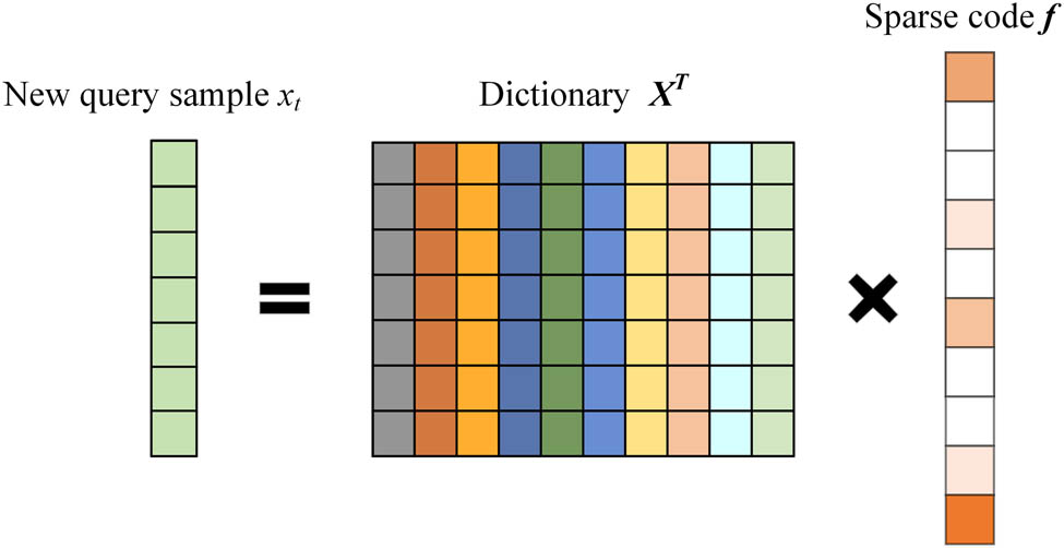
Schematic diagram of the SR.

Given a sample set X = [ x 1 , x 2 , ··· , x n ] T , where x k ∈ R m , m is the sample dimension, and n is the total number of samples. There exists a query sample x t and a pre-given set of samples X . It is customary to refer to the matrix X as an over-complete dictionary and x k as an atom. Finding the sparsest representation of the x t using a dictionary X requires minimizing the objective function:

where f is the sparse coefficient. The ‖ f ‖ 0 is the l 0 -norm, denotes the number p of nonzero entries in the vector f . x t can be represented linearly by satisfying x t ≈ X T f , where ‖ x t − X T f ‖ 2 ≤ ε .

2.2 Laplacian eigenmap (LE)

LE, as one of the representative nonlinear manifold learning methods, finds the low-dimensional embedding of the original data by preserving the similarity relationship between local points, which can better explain the geometric structure of nonlinear manifolds [15,19].

The steps for realization are as follows.

(1) Create a closest neighbor graph G using nodes as data points and edges generated by the k-NN method.

(2) Create a weight matrix W. Using a heat kernel, compute the edge weights w ij .

where σ ∈ R .

(3) Feature Mapping. To find the low-dimensional embedding, the eigenvalues and related eigenvectors are calculated. The eigenvalue decomposition is applied on the Laplace matrix L = D − W , i.e., Ly = λ Dy , where D is a diagonal matrix that satisfies D ii = ∑ j w ij , λ and y are the generalized eigenvalues and eigenvectors, respectively. The coordinates of the reconstructed space are the eigenvectors with the smallest d non-zero eigenvalues ( d ≪ M , where d is the number of low dimensions and M is the number of dimensions of the original high-dimensional space).

The traditional LE algorithm is only suitable for dealing with uniformly distributed flat manifolds, so for sparsely distributed or highly distorted manifolds [14], it is easy to mistakenly include the non-nearest neighbor points on the manifolds into the adjacency graphs, which incorrectly extracts the local geometric structures and interferes with the regression modeling. Meanwhile, the traditional LE algorithm, as an unsupervised dimension reduction method, lacks the use of label information, and different labels do not reflect the differences in weight assignment when constructing the neighborhood graph.

3.1 Supervised sparse weights (SSW)

Supervisory information significantly influences feature extraction [15]. Utilizing labels allows for the categorization of data with the same or similar labels, facilitating the extraction of differentiation information concealed within the original data. While the original LE algorithm can extract the low-dimensional embedding of high-dimensional data if all data points are situated on a single continuous manifold, BOF steel production process data typically exhibit various operational conditions, resulting in a complex nearest-neighbor relationship among data clusters. Assuming that data with identical or similar labels reside on distinct manifolds, the dataset manifests a multi-manifold structure, necessitating the extraction of information from corresponding manifolds for data with different labels [15,19].

Although raw LE adeptly captures and preserves local manifold shape information within the dataset, it falls short in segregating differently labeled data. To address this limitation, this section introduces an SSW module. Using label information, this module divides the historical dataset into relevantly and irrelevantly labeled subsets based on the characteristics of current query samples. Subsequently, it quantifies the relevance of each labeled set by assigning weights, thereby emphasizing label information.

Step 1: The current query sample x t is represented as a linear combination of the historical sample set X = [ x 1 , x 2 , ··· , x n ] T (where x k ∈ R m , m is the sample dimension, and n is the total number of samples) by SR, from which the sparse coefficient f is obtained, the larger the coefficient, the greater the degree of similarity of the query sample x t with the corresponding historical samples, whereby the sparse coefficient f is regarded as a similarity metric of x t with the historical sample set X as a result of the similarity measure. The sparsity coefficient f is calculated from equation (1).

Step 2: The labels of the historical samples corresponding to the index are extracted based on the non-zero terms in the sparse coefficient f and labe l 0 = [ l 1 , l 2 , ··· , l p ] , where p is the amount of non-zero terms in the sparse coefficient f .

Step 3: Removing duplicate labels gives the set of related labels labe l SSW = [ l 1 , l 2 , ··· , l q ] , q < p .

Step 4: The non-zero values of the sparsity coefficients corresponding to the statistics l k , k ∈ [ 1 , q ] are used as the degree of relevance W of different labels for the current query sample x t .

An SSW module is employed to disentangle historical sample sets from the influence of irrelevantly labeled data clusters, particularly in scenarios with complex distributions and multiple working conditions. This module quantifies the degree of association among relevantly labeled data sets, thereby mitigating the interference of irrelevant information on subsequent processing.

3.2 Trend match (TM)

While process data from distinct stages may exhibit varying numerical performances due to differences in initial conditions of the BOF and raw material batches, it is theoretically expected that the autocorrelation and inter-correlation among process variables within each stage adhere to intrinsic mechanistic relationships [22]. In the context of regression tasks, capturing similar trend samples is crucial for preserving their shared characteristics and production trends.

To address this, we introduce the TM module. This module identifies historical data with analogous trends in data sets associated with different relevant labels for the query sample x t by assessing the synchronization of change trends between samples, the similarity of underlying shapes, and comparisons of material values. Subsequently, it conducts modeling and prediction based on these evaluations. By analyzing and extracting similar trends, we can better understand and leverage their common characteristics, thereby enhancing the accuracy and reliability of the soft sensor model (Figure 3).

Figure 3

Schematic of SSW and TM.

Step 1: A quantitative evaluation of the degree of synchronization of the change trends and the degree of similarity of the base shapes between the historical samples and the query samples x t is made based on the Pearson correlation coefficient, which is calculated by the following equation:

where cov ( x i , x t ) is the covariance between x i and x t , x i is the i th history sample, x t is the query sample, and σ * is the standard deviation. The customized synchronization degree threshold C is determined by the following equation:

where N is the number of historical samples involved in the current sub-TM.

Step 2: The historical samples x i that satisfy ρ 1 ( x i , x t ) > C are formed into the initial filtered dataset. Considering the performance of different raw material ratios and furnace parameters on process data values, the difference in numerical performance is calculated on the basis of the initial filtration, and the samples with a difference less than the threshold value δ 1 are retained to form the filtered dataset X 1 with the following equation:

where δ 1 is the TM threshold and the value of the parameter is determined experimentally.

This results in a TM result, i.e., dataset X PF = [ x 1 , x 2 , ··· , x N 1 ] T , x i ∈ R m , i = 1 , 2 , ··· , N 1 < N . The matching result, X PF , contains samples in the historical dataset that have the same characteristics and trends as x t , reflecting similar physical properties, chemical compositions, furnace conditions, etc.

3.3 Manifold curvature analysis and adjacency matrix construction (MCA & AMC)

Traditional LE algorithms hinge on the accurate reflection of internal manifold structure by local neighborhood settings [14]. Oversized parameters are prone to eliminating small-scale manifold structures, leading to short-circuiting, while undersized parameters may result in manifold splitting [23]. The k-NN often generates distorted neighborhood structures for sparse and noisy data [23], exacerbating the short-circuiting phenomenon. Short-circuiting refers to the proximity of folding surfaces on the manifold, causing the search for nearest neighbors to include points from different folding surfaces rather than neighboring points on the manifold, thereby necessitating neighborhood optimization.

As depicted in Figure 4, the red circle illustrates the neighborhood range constructed by the traditional distance metric, wherein point a serves as the origin, and points c and d from the other folded plane are erroneously included. Even when employing solely geodesic distance as the distance metric, depicted in the gray section of the figure, point c, not residing in the same local linear plane, may still be considered a neighboring point. Hence, both metrics must collaborate in analyzing the curvature of the manifold in high-dimensional space to accurately construct neighborhoods. Given the non-uniform distribution of BOF steelmaking process data, the traditional k-NN can construct oversized neighborhoods in sparse regions. To address this, we introduce the MCA module in this section. This module incorporates geodesic distance proximity and subsequently filters out non-nearest neighbors after computing the curvature of local manifold shapes, enabling adaptive adjustment of neighborhood parameters to enhance model performance. Subsequently, the corresponding weights from the SSW module for each labeled dataset are merged and applied to each local neighborhood matrix. These matrices are then fused with the global neighborhood map to derive the fused neighborhood map for participation in dimension reduction.

Figure 4

Schematic diagram of MCA.

Step 1: The k neighborhood of any point x i ( i = 1 , 2 , ··· , N 1 ) in X PF is computed using Euclidean distances, thus forming the initial neighborhood graph.

Step 2: Solve for the geodesic distance d g ( x i , x j ) between any two points on the initial neighborhood map. If x i and x j are close neighbors of each other, then the geodesic distance is the Euclidean distance d e ( x i , x j ) , otherwise let d g ( x i , x j ) = ∞ as shown in equation (6), and N ( i ) is the neighborhood of x i .

Step 3: Using x h , iteratively compute all d g ( x i , x j ) .

Step 4: Adjust the neighborhood parameters based on the manifold curvature. Calculate the ratio of x i to the geodesic and Euclidean distances of the neighboring points as the manifold curvature with the following equation:

When λ is greater than the curvature analysis threshold δ 2 , x i and x j are considered to be on the same sub-manifold surface; otherwise, they are considered to be on different folded surfaces and non-manifold nearest neighbors, at this time, x j is removed from the neighborhood N ( i ) , which achieves the curvature analysis of the manifolds and optimization of the neighborhood parameters, and the resulting optimized curvature analyzed neighborhood graph G MCA is obtained.

Step 1: For the current query sample x t , from Definitions 1 and 2, we obtain different labeled sample clusters X PF i ( i = 1 , 2 , ··· , q ) and the corresponding weights W . The weights are applied to G X PF i , respectively, i.e., G X PF i = ω i * G X PF i . After that, G X PF i is sequentially connected head to tail in diagonal form and fused into a locally optimized neighborhood graph G L .

Step 2: The different labeled sets X PF i ( i = 1 , 2 , ··· , q ) obtained from Definitions 1 and 2 are sequentially merged to obtain the global similarity trend dataset, which serves as the input to the MCA module to obtain the globally optimized neighborhood graph G G .

Step 3: The globally optimized neighborhood graph G G and the locally optimized neighborhood graph G L are fused, i.e. G = G G + G L . The resulting fused neighborhood graph G is obtained and used as an input to the subsequent dimension reduction model.

5.1 Evaluation indicators

In order to evaluate the prediction performance, regression accuracy (RA), root mean square error (RMSE), and mean absolute percentage error (MAPE) are used as metrics in this article, among which RA is the most important, which indicates the prediction accuracy of the model for the test set within the allowable error. The formula for RA is as follows:

where N test is the number of test samples, y ∼ i and y i are the predicted and actual values of the i th output endpoint, respectively, and RE ( y ∼ i , y i ) is the conditional function, which outputs a 1 to indicate a prediction hit if the difference between the two outputs is within the range of tolerable error ( Te ) .

RMSE and MAPE are used to assess the regression model performance; the smaller the value, the better the model performance; the formula is as follows:

5.2 Data introduction and parameter setting

The experimental data were obtained from actual BOF steelmaking production data at a steel plant, with the target variables being the endpoint carbon content and temperature, i.e., the output variables. These samples were collected under different production conditions due to changes in raw material origins leading to quality differences between batches, adjustments in raw material ratios and furnace parameters, and changes in production conditions. First, the original dataset is checked and processed for missing data and outliers, and the corresponding samples are removed. Then, using the min–max scale, each variable to the range [0,1] using its minimum and maximum values, as shown in equation (14). Normalization is a preprocessing step crucial and effective for distance-based algorithms, equalizes the influence and importance of feature scales and thus prevents wide ranges or higher magnitudes from having a greater influence on learning [26]

where max ⁡ ( V ) and min ⁡ ( V ) are the maximum and minimum values of each variable in the original data, respectively. v i ′ is the normalized value of each variable in the range [ 0,1 ] .

A total of 3,000 furnace samples under normal operating conditions are collected in the experimental process, and 2,800 furnaces are randomly divided into 2,800 furnaces as the training set and 200 furnaces as the test set. As the raw process data contains a large number of redundant features. Therefore, based on previous research, 33-dimensional raw features are selected as input variables for the model according to feature importance [24,25] (Table 1).

Table 2 shows the optimal parameter values corresponding to the experiments.

5.3 Performance comparison of methods

5.3.1 Impact of TM thresholds and curvature analysis thresholds

The TM threshold δ 1 and the curvature analysis threshold δ 2 can have a great influence on the prediction accuracy. For the prediction of carbon content, the value interval of δ 1 is set to [ 0.0008 , 0.003 ] with a step size of 0.0001, and the value interval of δ 2 is set to [ 0.86 , 0.95 ] with a step size of 0.01, and the effects of different values of the thresholds on the results are analyzed, and the results are shown in Figure 5. As can be seen from the figure, the minimum value of RMSE occurs at δ 1 = 0.001 , δ 2 = 0.9 , when the RA reaches the highest. The graph shows a clear inverse relationship between RMSE and RA, which proves that the model prediction results fit the real values better and have better performance.

Figure 5

RMSE and RA results for different threshold values (carbon content). (a) Matching threshold δ 1 , (b) curvature analysis thresholds δ 2 .

For the prediction of temperature, the interval of δ 1 is set to [ 0.0004 , 0.001 ] with a step size of 0.0001, and the interval of δ 2 is set to [ 0.87 , 0.94 ] with a step size of 0.01, and the effect of different values of the thresholds on the results is analyzed, and the results are shown in Figure 7. As can be seen from the figure, the minimum value of RMSE occurs at δ 1 = 0.0006 , δ 2 = 0.88 , while the RA reaches the highest. In Figure 6 in the beginning stage RMSE and RA trends are similar, and then the tuning adjustment gradually shows an inverse relationship; this is due to the unreasonable parameter settings in the beginning stage, resulting in the model underfitting, cannot fit the data better, with the tuning, the model gradually improved.

Figure 6

RMSE and RA results for different threshold values (temperature). (a) Matching threshold δ 1 values for different modes, (b) different curvature analysis thresholds δ 2 .

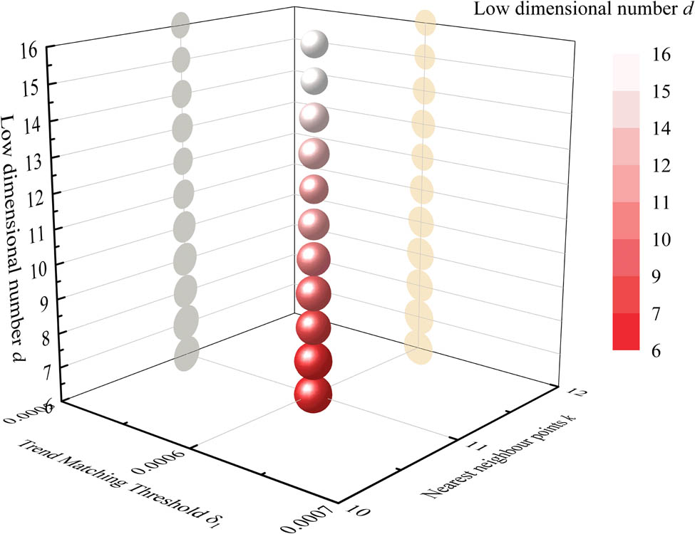
5.3.2 Impact of the number of nearest neighbor points

The LE algorithm is used as a local dimension reduction model, and the local geometry of the manifold shape is usually constructed based on the k-NN [15]. For carbon content prediction, the experiments were carried out in the interval [16,30] to determine the value of the number of nearest neighbor points k, and for temperature prediction, the experiments were carried out in the interval [10,24] to determine the value of the number of nearest neighbor points k, with a step size of 1. It was verified experimentally that, under the optimal settings of other parameters, the best performance of carbon content and temperature prediction was achieved with the values of the number of nearest neighbor points k being 24 and 11, respectively. Figures 7–10 show some of the experimental results. Table 3 shows some of the experimental results; the larger the sphere volume, higher the RA generated based on the corresponding parameters.

Figure 7

Effect of different numbers of nearest neighbor points k on the model. The larger the volume of the sphere in the figure, the higher the accuracy of the regression (carbon content).

Figure 8

Effect of different numbers of nearest neighbor points k on the model (carbon content).

Figure 9

Effect of different numbers of nearest neighbor points k on the model. The larger the volume of the sphere in the figure, the higher the accuracy of the regression (temperature).

Figure 10

Effect of different numbers of nearest neighbor points k on the model (temperature).

Table 3

Effect of different numbers of nearest neighbor points k and low dimensionality d on RA

Output variable	Nearest neighbor points ( k )	Low dimension number ( d )	RA (%)
Steel carbon content ( 10 ‒ 2 % )	19	7	72.50
	20	12	75.50
	21	13	78.50
	22	10	80.00
	23	10	77.50
	24	6	82.50
	25	7	79.50
	26	6	77.50
	27	6	78.50
	28	6	78.00
Steel temperature ( ° C )	10	6	76.50
	11	7	79.00
	12	6	74.00
	13	6	77.00
	14	9	71.00
	15	6	68.00
	16	7	68.50
	17	7	69.00
	18	6	65.50
	19	6	65.50

Bold values represent the best parameter settings and its experiment results.

From Figures 7 and 8, it can be seen that with the adjustment of the number of nearest neighbor points k, the RA of the model shows an increasing and then decreasing trend when predicting the carbon content and reaches a peak at k = 24. It shows that when k = 24, the dimension reduction results retain sufficient data structure information, so that the model can better capture the neighbor relationship between data points. As the k value continues to increase, the performance of the model begins to decline. Setting a larger value of the nearest neighbor point may increase the sensitivity of the noise, so that the low-dimensional embedding extraction results are greatly affected by the noise.

For Figures 9 and 10, as the number of nearest neighbor points k increases, the irrelevant information contained in the construction of the adjacency matrix gradually increases, and the RA tends to decrease significantly. With the increase of the number of neighboring points, the model will search for adjacent points more widely in the high-dimensional space, resulting in the points far away from each other participating in the construction of the adjacency matrix, which contains irrelevant information and reduces the RA.

Figure 11

Effect of different low dimension d on the model. The larger the volume of the sphere in the figure, the higher the accuracy of the regression (carbon content).

5.3.3 Impact of low dimension

Accurate parameter setting of low dimension can effectively retain the spatial geometric information of the data and improve the performance of the dimension reduction model. The experiments were carried out in the interval [6,16] to determine the value of the low dimension d, with a step size of 1. It was experimentally verified that the best prediction of carbon content and temperature with the optimal settings of the other parameters was achieved with the values of 6 and 7 for the low dimension d (Figure 11). Some of the results of the experiments are shown in Figures 12 and 13, where the greater the volume of the sphere, the greater the accuracy of the regressions generated based on the corresponding parameters (Table 4).

Figure 12

Effect of different low dimension d on the model. The larger the volume of the sphere in the figure, the higher the accuracy of the regression (temperature).

Figure 13

Results of ablation experiments: (a) carbon content, (b) temperature.

Table 4

Effect of different low dimension d on RA

Output variable	Low dimension number d	RA(%)
Steel carbon content ( 10 ‒ 2 % ) ( k = 24)	6	82.50
	7	77.50
	8	78.00
	9	76.50
	10	75.00
	11	76.00
	12	74.00
	13	76.00
	14	75.00
	15	73.50
	16	68.00
Steel temperature ( ° C ) ( k = 11)	6	78.50
	7	79.00
	8	72.50
	9	72.50
	10	69.00
	11	64.00
	12	59.00
	13	62.50
	14	59.50
	15	54.00
	16	55.00

Bold values represent the best parameter settings and its experiment results.

Table 5

Comparison of carbon content and temperature prediction result of ablation experiments

Output variables	Te	RA (%)
		TM_MCA&AMC	SSW_MCA&AMC	SSW_TM_AMC	The proposed method
Steel carbon content ( 10 ‒ 2 % )	0.01%	30.50	28.00	45.00	44.00
	0.02%	68.00	57.50	73.00	82.50
	0.03%	89.50	85.00	88.00	97.00
Steel temperature ( ° C )	5 ° C	41.00	31.50	45.00	54.50
	10 ° C	66.50	54.00	72.00	79.00
	15 ° C	84.50	75.00	88.50	89.00

Bold values represent the proposed method has the highest prediction accuracy compared with other algorithms.

5.3.4 Ablation experiment

Ablation experiments are conducted to validate the effectiveness of the proposed method. The regression model remains unchanged throughout the experiments, with model prediction performance contingent on the TM efficacy, neighborhood parameter optimization, and integration of SSWs. To assess the efficacy of the SWLSPP model, it undergoes ablation along the following lines:

1. Ablation of SSWs using the TM and MCA & AMC, which eliminates the interference of widely varying samples and manifolding non-nearest neighbors. However, it lacks the utilization of label information and differentiation between sets of differently labeled data. This ablation experiment is denoted as TM_MCA & AMC (Table 5).

2. For the ablation of TM, although the SSW module introduces labeling information, it lacks a mechanism to remove interference from irrelevant working condition sample information. This ablation experiment is denoted as SSWs_MCA & AMC.

3. For MCA ablation, the screening of non-nearest-neighbor points on the manifold is omitted. This ablation experiment is denoted as SSWs_TM_AMC.

Subsequent experiments are based on production process data, model parameters of methods adjusted to optimum values.

As depicted in Figures 13 and 14, the SSW_MCA&AMC configuration lacks the TM module to filter out samples with significant discrepancies. Consequently, the model extracts information with greater interference, resulting in the poorest fitting performance observed in Figure 14(b), particularly evident in larger errors during true predicted value jumps.

Figure 14

Comparison of results from ablation experiments (carbon content on the left, temperature on the right). (a) TM_MCA&AMC, (b) SSW_MCA&AMC, and (c) SSW_TM_AMC.

Conversely, TM_MCA&AMC effectively eliminates irrelevant information but fails to distinguish and analyze submanifold. It relies on the spatial geometric information of the overall dataset, neglecting the internal geometric structures unique to submanifold within each dataset labeled differently. This distinction is crucial for a comprehensive understanding of the dataset.

Meanwhile, SSW_TM_AMC augments information by incorporating features from the former two configurations. However, it overlooks the removal of non-nearest-neighbor points within neighborhoods, adversely impacting the model’s performance.

5.4 Experimental comparison results with other algorithms and analysis

In this section, the proposed SWLSPP algorithm is compared with other dimension reduction soft sensors including LE, Cosine Similarity and Jensen Shannon Divergence-Supervised Local Linear Embedding (CJS-SLLE), Supervised LE (S-LE₁), and LE with adaptive neighborhood parameters (S-LE₂). The parameters of all comparison algorithms have been tuned to the optimum in the experiments.

Analyzing Tables 6 and 7, Figures 15 and 16, reveal the following insights:

1. The LE algorithm, lacking mechanisms to reject irrelevant information and utilize labeling data, struggles to adapt to varying conditions when handling query samples with different working conditions. Consequently, it fails to accurately extract intrinsic data information, as evidenced in Figure 16(a).

2. The CJS-SLLE algorithm incorporates label information into similarity metrics, while S-LE₂ determines the number of nearest neighbors for each sample based on data density and adopts the geodesic line distance as the distance metric. However, both methods lack submanifold analysis of differently labeled data sets, impeding accurate extraction of intrinsic differences manifested in various labeled data sets. Although the modules for removing irrelevant information in CJS-SLLE and S-LE₂ effectively enhance model performance by 20 and 23% for carbon content prediction and 20 and 20.5% for temperature prediction, respectively. However, the neglect of difference information still leads to the limited improvement of fitting degree. as shown in Figure 16(b) and (d).

3. For the S-LE₁ algorithm, the average value of the distance between each sample and all samples is used as the threshold for judging the set of similar nearest neighbors and the set of dissimilar nearest neighbors when constructing the nearest neighbor graph, which does not take into account the similarity between the samples within a class and the differences between dissimilar samples very well, and at the same time, it will result in the increase of the computational cost, and the algorithm targets classification problems and performs poorly in regression tasks. Compared with S-LE₂, S-LE₁ lacks the consideration of folded surfaces and manifold curvature in the high-dimensional space and includes non-nearest neighbor points when constructing the nearest-neighbor map, which leads to the dispersion of the denser regions in the original data into multiple parts, affecting the accuracy of the dimension reduction results. From the experimental results, in the BOF steelmaking process data, compared with the original LE algorithm, S-LE1 improves by 16% and 11.5% when predicting carbon content and temperature, respectively.

4. According to Figures 15 and 16, the comparison between the real value and the predicted value of each soft sensor model shows that the SWLSPP model has the smallest error between the real value and the predicted value compared with the models of other methods, thus reflecting the effectiveness of the soft sensor modeling, and realizing the real-time accurate prediction of the carbon content and temperature of the endpoint of BOF steelmaking.

5. Table 7 shows the experimental results of the SWLSPP algorithm proposed in this article and other comparative algorithms for endpoint prediction, of the 78 furnace samples obtained. Due to the differences in data distribution between the new furnace dataset and the original training and test sets, the regression accuracies of some algorithms are reduced by 1.73–2.46% compared with Table 6. Meanwhile, the new dataset has a smaller number of samples, which may lead to the inability to fully evaluate the performance of the model.

Figure 15

Comparison results with other algorithms: (a) carbon content and (b) temperature.

Figure 16

Comparison results with other algorithms (carbon content on the left, temperature on the right). (a) LE, (b) CJS-SLLE, (c) S-LE1, (d) S-LE2, and (e) the proposed method.

References

[1] Yu, X. The simulation of multiphase flow behavior in BOF, Vol. 72, University of Science and Technology, Liaoning, 2018.Search in Google Scholar
[2] Han, M. and L. Jiang. Endpoint prediction model of basic oxygen furnace steelmaking based on PSO-ICA and RBF neural network, IEEE, 2010 International Conference on Intelligent Control and Information Processing, Dalian, China, 2010.10.1109/ICICIP.2010.5565236Search in Google Scholar
[3] He, F. and L. Zhang. Prediction model of end-point phosphorus content in BOF steelmaking process based on PCA and BP neural network. Journal of Process Control, Vol. 66, 2018, pp. 51–58.10.1016/j.jprocont.2018.03.005Search in Google Scholar
[4] Liu, Z., S. Cheng, and P. Liu. Prediction model of BOF end-point temperature and carbon content based on PCA -GA- BP neural network. Metallurgical Research & Technology, Vol. 119, No. 6, 2022, pp. 7039–7043.10.1051/metal/2022091Search in Google Scholar
[5] Wang, X., M. Han, and J. Wang. Applying input variables selection technique on input weighted support vector machine modeling for BOF endpoint prediction. Engineering Applications of Artificial Intelligence, Vol. 23, No. 6, 2010, pp. 1012–1018.10.1016/j.engappai.2009.12.007Search in Google Scholar
[6] Shao, W., Z. Ge, H. Li, and Z. Song. Semisupervised dynamic soft sensing approaches based on recurrent neural network. Journal of Electronic Measurement And Instrumentation, Vol. 33, No. 11, 2019, pp. 7–13.Search in Google Scholar
[7] Alakent, B. Online tuning of predictor weights for relevant data selection in just-in-time-learning. Chemometrics and Intelligent Laboratory Systems, Vol. 203, 2020, id. 104043.10.1016/j.chemolab.2020.104043Search in Google Scholar
[8] Yu, H. A just-in-time learning approach for sewage treatment process monitoring with deterministic disturbances, Yokohama, Japan, 2015.10.1109/IECON.2015.7392965Search in Google Scholar
[9] Yang, X., F. Yu, W. Pedrycz, and Z. Li. Clustering time series under trend-oriented fuzzy information granulation. Applied Soft Computing, Vol. 141, 2023, id. 110284.10.1016/j.asoc.2023.110284Search in Google Scholar
[10] Bader, J., D. Nelson, T. Chai-Zhang, and W. Gerych. Neural network for nonlinear dimension reduction through manifold recovery, Elke Rundensteiner, Cambridge, 2019.10.1109/URTC49097.2019.9660541Search in Google Scholar
[11] Zhang, X., Z. Chen, S. Yi, and J. Liu. Rapid detection of lignin content in corn straw based on Laplacian Eigenmaps. Infrared Physics & Technology, Vol. 133, 2023, id. 104787.10.1016/j.infrared.2023.104787Search in Google Scholar
[12] Liu, D., L. Wang, and J.A. Benediktsson. An object-oriented color visualization method with controllable separation for hyperspectral imagery. Applied Sciences-Basel, Vol. 10, No. 10, 2020.10.3390/app10103581Search in Google Scholar
[13] Qian, Q. Process monitoring and quality prediction of basicoxygen furnace steelmaking process based on functional data analysis, Vol. 169, University of Science and Technology, Beijing, 2023.Search in Google Scholar
[14] Li, Y. and L. Binghan. Self-regulation of neighborhood parameter for Laplacian eigenmaps. Journal of Fuzhou University (Natural Science Edition), Vol. 41, No. 2, 2013, pp. 153–157.Search in Google Scholar
[15] Li, B., Y. Li, and X. Zhang. A survey on Laplacian eigenmaps based manifold learning methods. Neurocomputing, Vol. 335, 2019, pp. 336–351.10.1016/j.neucom.2018.06.077Search in Google Scholar
[16] Kanghua, H. and W. Chunheng. Clustering-based locally linear embedding, Tampa, FL, USA, 2008.10.1109/ICPR.2008.4761293Search in Google Scholar
[17] Li, B., J. Liu, Z.Q. Zhao, and W.S. Zhang. Locally linear representation Fisher criterion, Dallas, TX, USA, 2013.10.1109/IJCNN.2013.6706985Search in Google Scholar
[18] Yang, L., H. Liu, and F. Chen. Soft sensor method of multimode BOF steelmaking endpoint carbon content and temperature based on vMF-WSAE dynamic deep learning. High Temperature Materials and Processes, Vol. 42, No. 1, 2023, id. 20220270.10.1515/htmp-2022-0270Search in Google Scholar
[19] Raducanu, B. and F. Dornaika. A supervised non-linear dimensionality reduction approach for manifold learning. Pattern Recognition, Vol. 45, No. 6, 2012, pp. 2432–2444.10.1016/j.patcog.2011.12.006Search in Google Scholar
[20] Wang, N. Research on class-preserving laplacian eigenmaps for dimensionality reduction, Harbin Engineering University, Harbin, China, 2017.10.1109/FSKD.2016.7603204Search in Google Scholar
[21] Zhang, J., J. Wang, and X. Cai. Sparse locality preserving discriminative projections for face recognition. Neurocomputing, Vol. 260, 2017, pp. 321–330.10.1016/j.neucom.2017.04.051Search in Google Scholar
[22] Ji, C. and W. Sun. A review on data-driven process monitoring methods: characterization and mining of industrial data. Processes, Vol. 10, No. 2, 2022, id. 335.10.3390/pr10020335Search in Google Scholar
[23] Wen, G. Dynamically determining neighborhood parameter for locally linear embedding. Journal of Software, Vol. 19, No. 7, 2008, pp. 1666–1673.10.3724/SP.J.1001.2008.01666Search in Google Scholar
[24] Xiong, Q. Study on the soft measurement method of carbon temperature at the end of blowing based on the integrated learning of converter steelmaking production process data, Vol. 83, Kunming University of Science and Technology, Kunming, China, 2021.Search in Google Scholar
[25] Zhao, A., H. Liu, F. Chen, X. Liu, and D. Zhang. Soft sensor method of endpoint carbon content and temperature of BOF steelmaking based on CJS-SLLE and just-in-time learning. Control Theory and Applications, 2023, Vol. 40, No. 10, pp. 1–11.Search in Google Scholar
[26] Tawakuli A., B. Havers , V. Gulisano , D. Kaiser, and T. Engel. Survey: time-series data preprocessing: a survey and an empirical analysis. Journal of Engineering Research, 2024.10.1016/j.jer.2024.02.018Search in Google Scholar
© 2024 the author(s), published by De Gruyter
This work is licensed under the Creative Commons Attribution 4.0 International License.
Articles in the same Issue
- Research Articles
- De-chlorination of poly(vinyl) chloride using Fe2O3 and the improvement of chlorine fixing ratio in FeCl2 by SiO2 addition
- Reductive behavior of nickel and iron metallization in magnesian siliceous nickel laterite ores under the action of sulfur-bearing natural gas
- Study on properties of CaF2–CaO–Al2O3–MgO–B2O3 electroslag remelting slag for rack plate steel
- The origin of {113}<361> grains and their impact on secondary recrystallization in producing ultra-thin grain-oriented electrical steel
- Channel parameter optimization of one-strand slab induction heating tundish with double channels
- Effect of rare-earth Ce on the texture of non-oriented silicon steels
- Performance optimization of PERC solar cells based on laser ablation forming local contact on the rear
- Effect of ladle-lining materials on inclusion evolution in Al-killed steel during LF refining
- Analysis of metallurgical defects in enamel steel castings
- Effect of cooling rate and Nb synergistic strengthening on microstructure and mechanical properties of high-strength rebar
- Effect of grain size on fatigue strength of 304 stainless steel
- Analysis and control of surface cracks in a B-bearing continuous casting blooms
- Application of laser surface detection technology in blast furnace gas flow control and optimization
- Preparation of MoO3 powder by hydrothermal method
- The comparative study of Ti-bearing oxides introduced by different methods
- Application of MgO/ZrO2 coating on 309 stainless steel to increase resistance to corrosion at high temperatures and oxidation by an electrochemical method
- Effect of applying a full oxygen blast furnace on carbon emissions based on a carbon metabolism calculation model
- Characterization of low-damage cutting of alfalfa stalks by self-sharpening cutters made of gradient materials
- Thermo-mechanical effects and microstructural evolution-coupled numerical simulation on the hot forming processes of superalloy turbine disk
- Endpoint prediction of BOF steelmaking based on state-of-the-art machine learning and deep learning algorithms
- Effect of calcium treatment on inclusions in 38CrMoAl high aluminum steel
- Effect of isothermal transformation temperature on the microstructure, precipitation behavior, and mechanical properties of anti-seismic rebar
- Evolution of residual stress and microstructure of 2205 duplex stainless steel welded joints during different post-weld heat treatment
- Effect of heating process on the corrosion resistance of zinc iron alloy coatings