Experimental and numerical analysis of temperature distributions in SA 387 pressure vessel steel during submerged arc welding
-
Murat Makaraci

 and
Mert Turgut Senol
and
Mert Turgut Senol

Abstract
The present study aims to explore experimental investigations and numerical simulations for temperature distributions at heat-affected zones within SA 387-Gr.11-Cl.2 steel during the submerged arc welding (SAW) process. Experimental endeavors entailed welding steel plates under controlled conditions, precisely measuring temperatures at key locations by thermocouples. A special program based on 3D Goldak’s double ellipsoidal model was developed in ANSYS Parametric Design Language for moving heat source calculations in the finite-element analysis (FEA). For welding an 8 mm thick plate with one pass, the suitable parameters were found to be 600 A current, 31 V voltage, and 10 mm·s−1 welding speed. The experimental cooling periods were found to be slower than predicted by FEA. When temperature distributions were compared between experimental and FEA results, an average variation of 1.88% at peak temperatures and 11.8% at completion time was observed. The results showed the temperature distribution at various time steps, illustrating the transient nature of the welding process. The results highlight the capacity of the FEA model to predict temperature profiles during SAW accurately, presenting a potent tool for optimizing welding parameters without extensive trial and error.
Nomenclature
- a, b
-
geometric parameter of double ellipsoid
- c
-
specific heat
- c f, c r
-
dimensions of the front and rear semi-ellipsoidal heat source
- f f, f r
-
fractions of heat flux deposited, corresponding to the front and rear quadrants
- h
-
convection coefficient of heat transfer
- I
-
current applied to weld
- k x , k y
-
thermal conductivity in x and y directions
- q in
-
rate of internal heat generation
- q out
-
rate of latent heat generation
- t
-
time
- T
-
temperature
- T ∞
-
ambient temperature
- TC n
-
thermocouple location at n
- Q
-
heat input
- V
-
voltage applied to weld
- ε
-
emissivity, engineering strain
- η
-
efficiency of the welding process
- ρ
-
density
- σ
-
Stefan–Boltzmann constant, stress
1 Introduction
The design and manufacturing of pressure vessels for high-temperature applications are of paramount importance in ensuring the safety and reliability of industrial processes. These vessels play a critical role in containing substances under extreme thermal conditions, where any structural failure could lead to catastrophic consequences. Precision in design and adherence to rigorous manufacturing standards are essential to prevent material degradation, maintain structural integrity, and guarantee the longevity of these vessels, safeguarding both industrial operations and human safety.
SA 387 Grade 11 Class 2, a steel grade designed for use in pressure vessels under elevated temperature conditions, finds extensive application across various industrial sectors. Its effectiveness is particularly pronounced in the oil, gas, and petrochemical industries, where it excels in storing liquids and gases at elevated temperatures. The elevated chromium levels in this material confer remarkable resistance to both corrosion and oxidation, a vital attribute in applications involving sour gases [1]. In a multitude of industries, the SA 387 GR.11 CL.2 Plate is the preferred choice for elevated temperature service due to its capability to endure high operational temperatures at 600°C. This plate’s high chromium content imparts outstanding resistance to oxidation and corrosion, making it indispensable for sour gas applications. Its precise manufacturing techniques within the industry result in a product endowed with exceptional qualities, making it a staple in global industries across diverse applications. These qualities encompass impressive tensile strength, robustness, precise dimensional accuracy, impeccable surface finishes, weldability, extended service life, flexibility, durability, and the ability to withstand substantial loads. Furthermore, it exhibits full resistance to pitting, crevice corrosion, and stress corrosion cracking [2]. The chemical composition and the mechanical properties of the steel SA387 are given in Tables 1 and 2, respectively.
Chemical composition of SA387 GR.11 CL.2 plate
| C | 0.05–0.17 |
| Mn | 0.40–0.65 |
| P | 0.025 |
| S | 0.025 |
| Si | 0.50–0.80 |
| Cr | 1.00–1.50 |
| Mo | 0.45–0.65 |
Mechanical properties of SA 387 GR.11 CL.2 plate
| Tensile strength | 70–90 ksi, 485–620 MPa |
| Yield strength | 45 ksi, 310 MPa |
| Elongation in 200 mm (%) | 18 |
| Elongation in 50 mm (%) | 22 |
Submerged arc welding (SAW) is a widely employed process for coalescing metals through the application of electric arcs and the use of granular flux to shield the arc. SAW is particularly prevalent in heavy fabrication industries, although its limited mobility necessitates a relatively fixed workstation setup. The process involves the continuous deposition of flux to protect the arc and the workpiece, with the flux often serving to augment alloying elements introduced by the filler wire. SAW holds immense significance in the fabrication of pressure vessels.
This specialized welding technique involves immersing the welding arc and the joint in a granular flux, creating a controlled environment that offers several crucial advantages for pressure vessel construction. These are listed in the following.
1.1 Exceptional weld quality
SAW consistently produces high-quality, defect-free welds. Submerging the arc and weld pool in a layer of granular flux shields the weld from atmospheric contamination, reducing the risk of defects such as porosity and inclusions. This results in welds that meet stringent quality standards and ensures the pressure vessel’s reliability.
1.2 Efficiency and productivity
SAW is highly efficient and can be automated, making it well suited for high-volume pressure vessel production. Welding speed is in the order of 0.01 m·s−1. This efficiency reduces labor costs and significantly accelerates the welding process, a crucial factor when constructing pressure vessels for industries with tight production schedules. The deposition rate of filler material can be observed to be higher when compared to other methods.
1.3 Precise heat control
Effective management of heat input during welding is crucial for pressure vessels, especially those intended for high-temperature service. SAW is a continuous, controlled process that allows for precise heat management, reducing the risk of distortion and maintaining the desired material properties.
1.4 Deep and uniform penetration
SAW provides deep and consistent weld penetration, ensuring a strong and reliable bond between the base materials. This is essential for maintaining the structural integrity of pressure vessels subjected to high internal pressures and temperatures.
1.5 Minimal heat-affected zone (HAZ)
SAW creates a narrow HAZ in the surrounding material, minimizing the risk of thermal distortion and preserving the mechanical properties of the base metal. This is crucial for pressure vessels as it helps maintain the material’s strength and resistance to fracture.
1.6 Code and standard compliance
Many pressure vessels are designed and constructed to adhere to rigorous industry codes and standards, such as the ASME Boiler and Pressure Vessel Code. SAW has a reputation for consistently producing high-quality welds and facilitates compliance with these regulations, ensuring that the vessels meet safety and performance requirements.
The described process operates within inherent constraints on mobility, encompassing several key elements. First, movement along the weld line is essential, requiring the welding head, gun, nozzle, and associated components to traverse either longitudinally or radially, often with the workpiece positioned flat or horizontally. Additionally, flux application and delivery occur from a fixed location, representing a critical aspect of the operation. Figure 1 offers a schematic representation and an explanatory overview of the process. The figure illustrates a single arc and provides a cutout view displaying the completed weld.
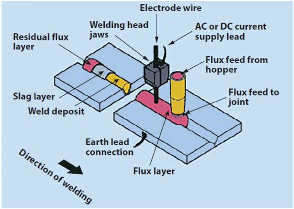
Schematic representation of the SAW process.
From the uppermost region extending down to the weld interface, the composition consists of distinct layers. At the uppermost layer lies the residual flux, which remains unconsumed during the welding process, serving solely to provide comprehensive coverage over the underlying weld zone. Directly beneath this protective blanket of flux lies the solidified slag, resulting from the fusion of the flux layer during the welding operation. Finally, the actual weld is situated below the slag layer. It is noteworthy to observe the precise positioning of the welding head, the flux feed hopper, and the direction of the welding operation. The power supply and electrode wire are seamlessly guided through the welding head, while the flux is effectively dispensed through the dedicated hopper mechanism [3].
In summary, SAW is of supreme importance in the fabrication of pressure vessels due to its ability to deliver high-quality, efficient, and reliable welds. Its capacity to maintain weld integrity, reduce defects, and adhere to industry standards makes it an indispensable welding technique for ensuring the safety and functionality of pressure vessels across various critical applications.
This study delves into the transient thermal characteristics of SA387-Gr.11-Cl.2 steel during SAW and investigates their temporal evolution. Some recent numerical and experimental efforts have been attempted [4–35], and Sepe et al. reviewed some of these findings in their work [36]. Temperature distribution can provide information about residual stress that may lead to material failures under unexpected operational conditions. To obtain accurate temperature distribution, one has to perform experiments that are time consuming and costly. To authors’ knowledge, the finite-element analysis (FEA) procedure has been applied for the first time using Goldak’s double ellipsoidal method on SA 387 steel. For this matter, an ANSYS Parametric Design Language (APDL) code is written to incorporate Goldak’s formulation. One can utilize the findings of this research without undergoing costly experiments. The current research presents a combination of meticulous experimental measurements and a developed numerical FEA characterizing the thermal behavior of SAW joints in this critical material. It addresses well the nonlinearity of complex thermal dynamics inherent to this material during the welding process. Numerical finite element (FE) simulations of temperature distributions, incorporating a 3D Goldak’s double ellipsoid heat source model integrated into the general-purpose FE software ANSYS, facilitated by a custom-developed code in APDL language. Subsequently, experimental measurements are conducted with various thermocouples (TC) strategically positioned on the specimen, enabling a comprehensive comparison between experimental and numerical data.
2 Materials and methods
In our experimental investigation, we utilized ASME SA 387 Grade 11 Class 2 steel as the base material. This steel grade is commonly employed in applications requiring resistance to elevated temperatures, notably within industries such as oil, gas, and petrochemicals. Two plates, both composed of the aforementioned material, were subjected to welding. The specimen dimensions measured 100 mm in length, 100 mm in width, and 8 mm in thickness, as depicted in Figure 2.
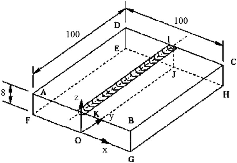
Workpiece dimensions.
Single-pass SAW was performed on a fully automatic welding machine, with welding parameters such as current, voltage, root gap, welding time, and welding speed carefully controlled. To identify the optimal current value, we conducted experiments with current as the variable, while maintaining voltage, welding speed, and the length of stick-out at constant values. Initial experiments involved a series of trial-and-error tests with varying current values, specifically 430, 530, 560, and 600 A. Subsequently, the most suitable current value for welding was determined to be 600 A. To determine the most suitable current value, a series of experiments were conducted with varying current levels. The selected welding parameters for the experiments are detailed in Table 3.
SAW Parameters used in the experiments
| Current (A) | 600 |
| Voltage (V) | 31 |
| Root gap (mm) | 1 |
| Welding time (s) | 10 |
| Welding speed (m·s−1) | 0.1 |
Sample parts were initially cut using a plasma-cutting machine and subsequently subjected to thorough cleaning through grounding. Before welding, a preheating process was applied to the area adjacent to the weld zone, maintaining it within a specified temperature range referred to as the preheating temperature. This temperature varies based on factors such as the chemical composition of the base metal, heat input, hydrogen diffusion, and base plate thickness. Typically, the preheating temperature range for SA387 GR 11 Class 2 steels falls between 150 and 200°C [37,38]. Preheating was accomplished using a localized heat treatment unit and electrical resistances. To prevent any unintended movement of metals during the welding process, the parent metal was securely clamped, and welding backing plates were affixed at the beginning and end of the component, as depicted in Figure 3.

Clamping of the workpiece and setup of the SAW process.
Before initiating the SAW process, the test plate pair was firmly attached using gas tungsten arc welding (GTAW) from both upper and lower sections to prevent sample displacement during welding. For tack welding and weld-backing-plate placement, the GTAW process was executed using an Esab Origo Tig 3001i TIG welding machine with a power source of 300 A. A filler metal ER80S-B2 with a 2.4 mm diameter was employed for the GTAW process. The gas composition consisted of 99.997% argon, delivered at a flow rate ranging from 11 to 16 L·min−1. The SAW welding machine used in the experiments is shown in Figure 4.
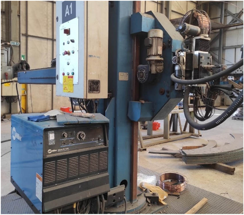
SAW machine utilized in the experiments.
Backing material, situated at the root of a weld joint, serves the purpose of supporting molten weld metal and facilitating complete joint penetration. To protect the bottom surface of the workpiece from damage, a ceramic protector was affixed to it. SAW was performed utilizing a 1,000 A constant potential power source, specifically the Miller Sub arc DC 1000. A filler metal with a 3.2 mm diameter, conforming to AWS A5.23: F8P2-EB2-B2, was used, along with Esab Flux 10.62 agglomerated fluoride-basic flux [39]. The chemical composition of the filler metal is detailed in Table 4.
Chemical composition of AWS A5.23 F8P2-EB2-B2 [39]
| C | Mn | Si | P | S | Cr | Mo | Cu |
|---|---|---|---|---|---|---|---|
| 0.09 | 0.80 | 0.25 | 0.013 | 0.008 | 1.10 | 0.45 | 0.03 |
Temperature data were recorded using K-type TC wires, which are composed of chrome/nickel aluminum TC wire insulated with high-temperature glass braid. These measurements were facilitated by a Honeywell eZtrend paperless recorder equipped with six directly connected analog inputs. To ensure accurate measurements, the TC wires were affixed directly to the workpiece using a “TC Attachment Unit.” Five TCs were strategically placed for temperature measurement, with their corresponding attachment points depicted in Figure 5, while the geometric specifics are provided in Figure 6.
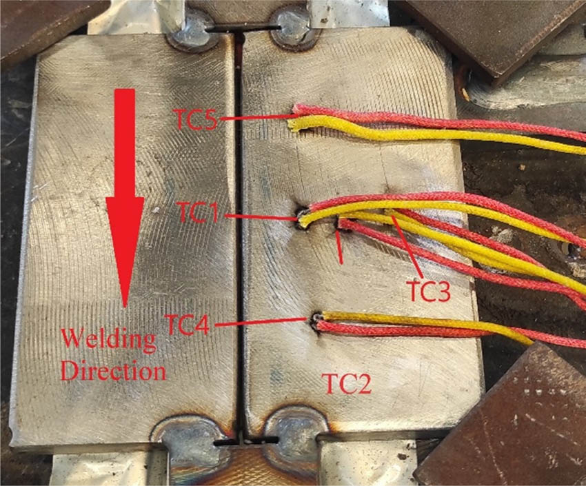
TCs attached to the workpiece.
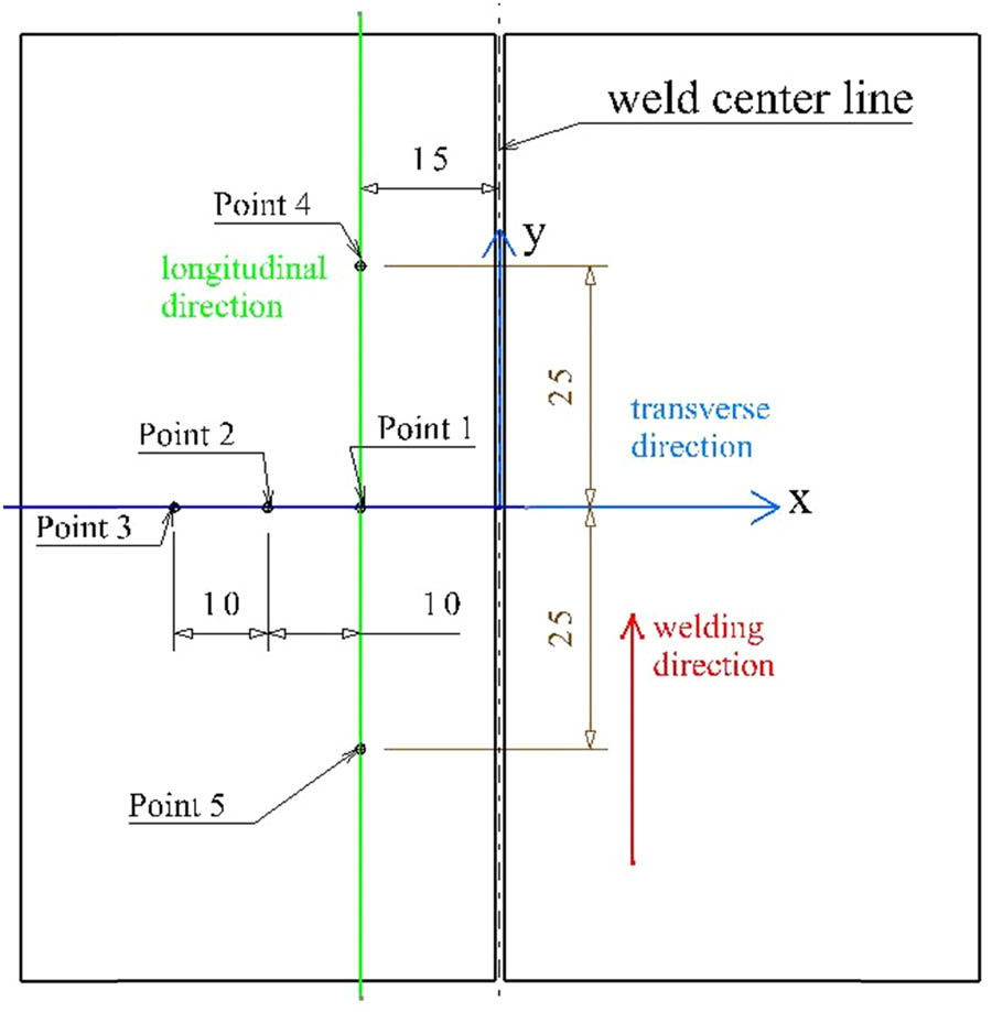
Geometric data of TC measurement points.
Among these, TC1, TC4, and TC5 were situated 15 mm away from the weld centerline of the weld joint, while TC2 and TC3 were positioned 10 mm in the x-direction away from TC1. The specific coordinates for the placement of these TCs are referenced from the chosen coordinate system, which was centered at the midpoint of the part.
Access to the recorded data stored in the Digital Honeywell Recorder was facilitated with the Pro version of TrendViewer, an application developed by Honeywell. These data were then conveniently made accessible in MS Excel format for analysis and subsequent processing.
2.1 Numerical model development for FEM
In the domain of arc welding, the distribution of temperature plays a pivotal role in influencing residual stress, distortion, and the strength of a welded structure, thereby affecting the overall quality of the resultant structure. Consequently, understanding the temperature evolution during welding has become a crucial research focus in recent decades. The utilization of mathematical models to predict welding temperatures has gained prominence, given the often prohibitively expensive nature of experimental predictions. Among the various mathematical models, numerical modeling, specifically FEA, has emerged as the preferred industry method for simulating and monitoring welding processes due to its computational efficiency and speed [40].
In this study, we developed an FEA model using ANSYS 2020 R2, incorporating the Goldak double ellipsoidal heat source model to predict the thermal cycle of SAW accurately. The primary objective of this research is to create an FEA model capable of reliably predicting the SAW thermal cycle with high accuracy compared to experimental results. The numerical simulation of the welding process was conducted through transient thermal analysis within ANSYS 2020 R2. The Goldak double ellipsoidal formulation was coded using the APDL to simulate characteristics of the SAW process applied to high-temperature resistive, anti-corrosive pressure vessel steel.
In the preprocessing phase of FEA, the material properties essential for accurate modeling can be categorized into two groups: thermal properties and physical properties of SA 387 GR 11 Class 2 steel [40]. Thermal properties include thermal conductivity (W·m−1·°C) and specific heat (J·kg−1·°C), while physical properties encompass density (kg·m−3), Young’s modulus (GPa), and thermal expansion (W·m−1·°C), as shown in Table 5. It is important to note that these material properties were assumed to vary with temperature during the heating and cooling cycles. When data were not available, an extrapolation procedure was utilized.
Thermal properties of SA 387Gr 11 Cl.2 [41]
| Temp. | Density | Thermal conductivity | Specific heat | Enthalpy |
|---|---|---|---|---|
| (°C) | (kg·m−3) | (W·m−1·°C) | (J·kg−1·°C) | (J·m−3 × 10⁸) |
| 20 | 7,750 | 41 | 470 | 0.1 |
| 100 | 7,750 | 40.6 | 487 | 3.6 |
| 200 | 7,750 | 40.1 | 529 | 7.2 |
| 300 | 7,750 | 38.7 | 564 | 11 |
| 400 | 7,750 | 36.8 | 605 | 15 |
| 500 | 7,750 | 34.8 | 666 | 19.8 |
| 600 | 7,750 | 32.8 | 760 | 25 |
| 700 | 7,750 | 29.1 | 1,008 | 30 |
| 800 | 7,750 | 27.5 | 803 | 37 |
| 900 | 7,750 | 24 | 650 | 45 |
| 1,000 | 7,750 | 20.1 | 650 | 50 |
| 1,100 | 7,750 | 15.8 | 650 | |
| 1,200 | 7,750 | 11.1 | 650 | |
| 1,300 | 7,750 | 6 | ||
| 2,500 | 90 |
Acquiring precise temperature-dependent material properties data from the literature proved to be challenging. Consequently, for this study, the material properties of SA 387 were adopted as provided by the ASME Boiler and Pressure Vessel Code, specifically ASME BPVC.II.D.M-2021. The SA 387 GR 11 Class 2 material in question is characterized as 1¼Cr–½Mo carbon–molybdenum steel.
A three-dimensional FE model was developed to address the engineering challenge at hand. The model focused on simulating SAW of single-sided single-pass butt joints, and it was created and analyzed using Space Claim 2020 R2 and ANSYS Mechanical Workbench. The model’s accuracy is contingent on parameters such as element size, node count, and time step size. Increasing the number of nodes not only enhances model precision but also extends the processing time.
In this thermal analysis, the chosen element type was SOLID90, as shown in Figure 7. SOLID90 represents an advanced iteration of the 3D eight-node thermal element, SOLID70. This element comprises 20 nodes, each with a single degree of freedom related to temperature. The use of 20-node elements with compatible temperature shapes is particularly well suited for modeling curved boundaries. Consequently, the 20-node thermal element finds applicability in both 3D steady state and transient thermal analyses. The FE model was composed of 358,743 nodes and 80,800 elements, with an element size of 0.001 m. The isometric view of the meshed model is shown in Figure 8.
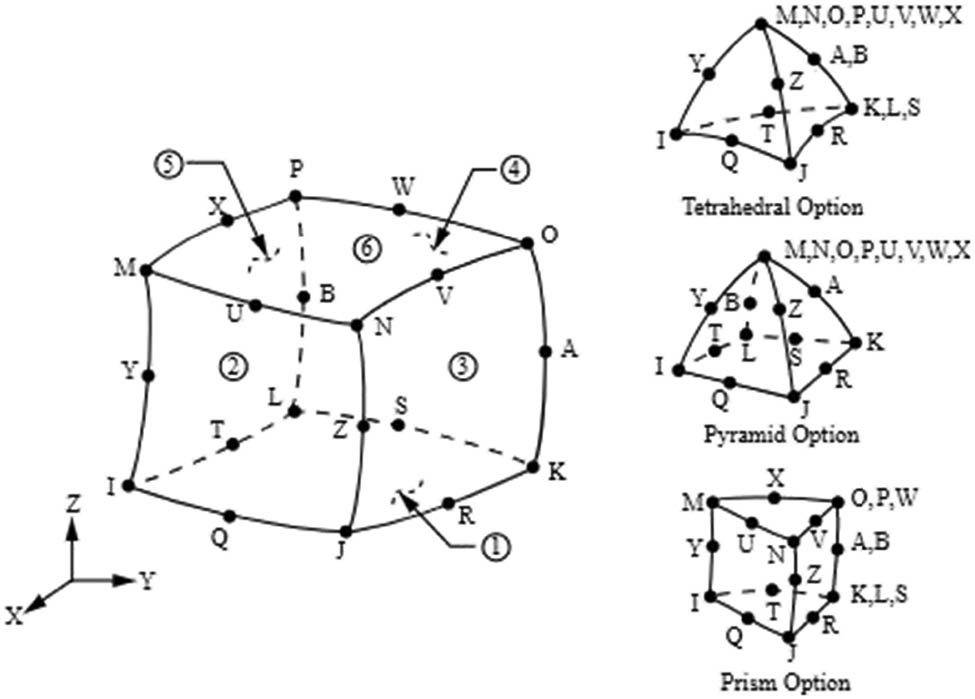
Nodal representation of SOLID90 thermal element.

Isometric view of the meshed model.
Boundary conditions encompass a set of loadings, constraints, and contact conditions that define the simulation’s state in a particular design configuration. Before initiating transient thermal and static structural analyses, these boundary conditions must be systematically applied to the model through a sequence of experimental procedures. Within this set, several loading and constraint conditions are expressed mathematically. In thermal analysis, the boundary conditions involve aspects such as convection and specific heat flux, while static structural analysis incorporates forces, moments, and displacements [42].
Heat transfer mechanisms are indeed commonly categorized into three main modes: conduction, convection, and radiation, as shown in Figure 9. The heat flow at the weld joint plays a critical role in the melting process. A substantial amount of heat at the source is emitted through radiation from the high-temperature region’s surface and the melt pool’s surface. Simultaneously, a significant portion of the heat required for melting is conveyed to the material through processes of conduction and convection [43].
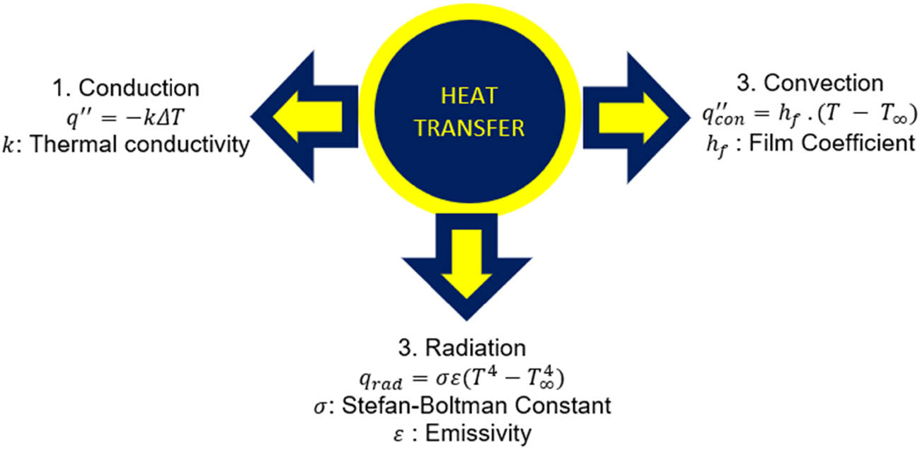
Heat transfer modes during the welding process.
In thermal analysis, the transient temperature field (T) within the welded component is a function of time and spatial coordinates (x, y). This field is governed by a non-linear heat transfer equation:
where q in represents the rate of internal heat generation, and q lat denotes the rate of latent heat generation. The coefficients of thermal conduction in the x and y directions are represented as k x and k y , respectively. Additionally, c signifies the specific heat, and ρ represents the density of the plate material. In this model, we accounted for the latent heat released during phase transformations. As a result, an enthalpy formulation was adopted. Enthalpy encapsulates all the necessary data for calculating latent heat release, with the exception of thermal conductivity and density, as documented in previous research [44].
Heat transfer during welding involves the initial application of the heat source to the welded component, followed by cooling through a combination of convection and radiation. In this analysis, we did not consider forced convection. The heat flux on the surfaces of the welded plate due to convection and radiation is expressed by the following equations:
where T ∞ represents the ambient temperature, and T signifies the boundary temperature exposed to the environment. The Stefan–Boltzmann constant, denoted as σ (5.67 × 10⁸ W·m−²·°C−4), and ε, which represents emissivity, were included in the equations. The convection coefficient was defined as h = 100 W·m−² for all surfaces of the plate, except for the top surface, which was considered insulated when the welding torch was directly above it. All analyses were conducted, taking into account the temperature-dependent thermal properties of the base metal. The model’s formulation was based on the following assumptions:
The initial temperature of the test plate was set at 150°C.
The ambient temperature of the weldments was maintained at 20°C.
Thermal properties of the material, such as specific heat, enthalpy, and conductivity, are temperature-dependent, as shown in Table 5.
Physical properties of the material, including elastic modulus and thermal expansion, are temperature-dependent.
Density is a constant value of 7,750 kg·m−³.
The convection heat transfer coefficient was set at 10 W·m−²·°C, and for radiation, an emissivity value of 0.9 was used.
The top face and side surfaces of the welded part were taken as insulated. Heat losses due to radiation and convection were considered only for the bottom surface of the welded parts.
Forced convection was not taken into account.
Element birth and death were not considered.
Boundary conditions for transient thermal analysis are shown in Figure 10.
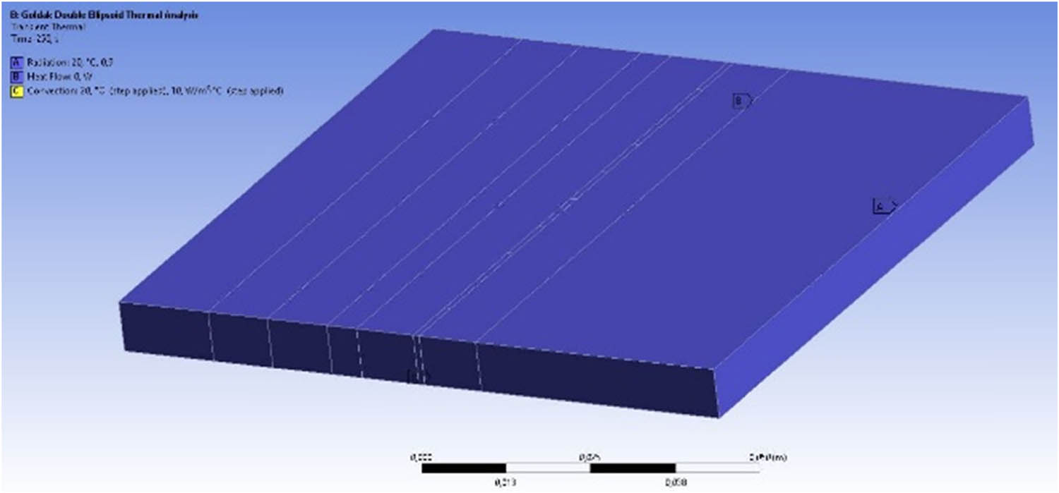
Boundary conditions for transient thermal analysis.
2.2 Moving heat source model
The modeling of a moving heat source represents an atypical transient thermal process. In our approach, the moving heat source is modeled using ANSYS 2020 R2 with APDL codes. The objective is to move the heat source continuously at minor increments while maintaining constant heat energy. During this dynamic process, the center of the heat source changes over time. This is achieved by modifying the parameters within the function that describes the heat source’s locations as a function of time. To develop the temperature distribution in our analysis, we employ Goldak’s double ellipsoidal heat source model, as depicted in Figure 11 [45]. This approach successfully represents the heat flux generated by the welding torch in SAW. A general FE solution scheme for heat transfer problems in the welding process is illustrated in Figure 12 [46], and accordingly, a transient temperature simulation has been performed by the authors to show numerical stability and experimental validation purposes [39].
![Figure 11
Schematic diagram for Goldak’s double ellipsoid model [45].](/document/doi/10.1515/htmp-2024-0009/asset/graphic/j_htmp-2024-0009_fig_011.jpg)
Schematic diagram for Goldak’s double ellipsoid model [45].
![Figure 12
Flow diagram for thermal FEM procedure [46].](/document/doi/10.1515/htmp-2024-0009/asset/graphic/j_htmp-2024-0009_fig_012.jpg)
Flow diagram for thermal FEM procedure [46].
The power density within our developed model is distributed throughout a volume, spanning both the front and rear quadrants of the heat source is
The heat flux equation for the heat source model or welding arc in the front quadrant is expressed as follows:
The heat flux equation for the heat source model or welding arc in the rear quadrant is as follows:
where, a, b, c f, and c r represent the geometric parameters, where c f and c r denote the dimensions of the front and rear semi-ellipsoidal heat sources, and f f and f r represent the fractions of heat deposited, corresponding to the front and rear quadrants’ heat apportionment of the heat flux. It is important to note that f f + f r equals 2. Q represents the heat input, while x, y, and z are the coordinates of the heat flux. Additionally, η stands for the efficiency of the welding process [47].
The Goldak double-ellipsoidal model is employed to characterize the volumetric heat flux in arc-welding processes. This model is renowned for its widespread use and popularity in simulating arc-welding procedures. To implement the Goldak double ellipsoid model within the ANSYS environment, specific APDL commands are required.
f f and f r parameters are calculated using the following formulas:
In the experiment conducted for this study, the energy input rate Q (I = 600 A, V = 31 V, η = 0.8) and the welding speed were set at 15,000 W and 0.01 m·s−1, respectively. Through an examination of the weld part and cross-section, as illustrated in Figures 12–15, heat source parameters were determined as follows: a = 10 mm, b = 8 mm, c r = 10 mm, c f = 30 mm (3 × c r), f f = 0.5, and f r = 1.5.
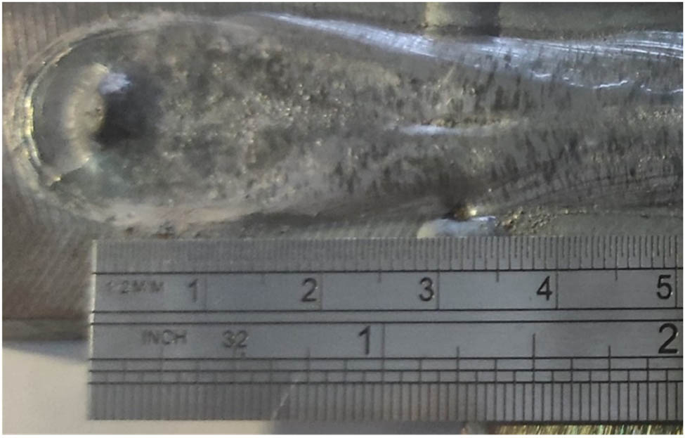
Goldak’s double ellipsoidal parameters view on the test plate.

Goldak’s double ellipsoidal parameters: the view of bead width (value for parameter “a”).
All measured parameters for the double ellipsoidal model are presented in Table 6. These values were utilized in the development of the FEM code. Table 7 provides a summary of the welding parameters used in the SAW process, which are necessary inputs for the transient FE solution. Typical efficiency values for various welding processes are listed in Table 8, with SAW being reported as 91–99% [38]. However, during the numerical integration of FE iterations, the solutions exhibited divergence, indicating numerical instability. This challenge was resolved by reducing the efficiency to a level of η = 0.8, resulting in convergent solutions in the FE calculations. Numerical instability may arise due to high heat input. For this reason, we take 0.8 efficiency values in the calculations of heat input. Heat input is described by efficiency × voltage × current. Numerical results and experimental results give near values at this efficiency.
Measured model parameters used in FEA (all dimensions are in mm)
| a | b | c f | c r | f f | f r |
|---|---|---|---|---|---|
| 10 | 8 | 10 | 30 | 0.5 | 1.5 |
Welding parameters used in SAW
| Power (A) | 600 |
| Voltage (V) | 31 |
| Heat input Q = I × V × ɳ (W) | 15,000 |
| Progression speed (mm·s−1) | 10 |
Efficiency ranges for various welding processes [38]
| Welding process | ɳ |
| GTAW Ar, steel | 25–75 |
| GTAW He, Al | 55–80 |
| GTAW Ar, Al | 22–46 |
| SMAW steel | 66–85% |
| GMAW Ar, steel | 66–70 |
| SAW steel | 91–99 |
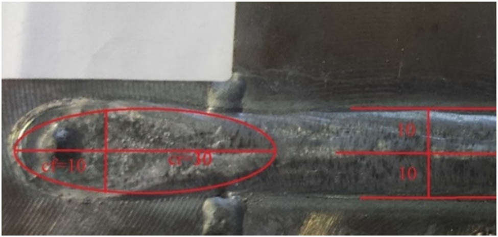
Goldak’s double ellipsoidal parameters view on test plate: a, c r, and c f.
3 Results and discussion
The primary objective of this study is to develop a 3D-FEA model capable of predicting the SAW thermal cycle with higher accuracy compared to experimental work. Transient temperature distribution analysis was conducted using ANSYS 2020 R2 software. The 3D FE model was executed on an Intel(R) Core(TM) i7-10750H CPU @ 2.60 GHz with 16 GB RAM. The analysis required approximately 20 h of CPU time. Predicted temperatures were then compared with temperatures obtained from experiments. In the experimental phase, temperature distribution was measured using chrome/nickel aluminum TCs with a diameter of 0.71 mm. Temperature history during the welding process was recorded using a Honeywell Eztrend temperature recorder, and the recorded temperature data were exported to Excel for analysis.
The FEM simulation results depicting the progression of temperature distributions at the top of the plate, where welding was performed along the welding center direction, are presented in Figures 16–20. These figures correspond to elapsed times of 3, 6, 10, 30, and 250 s, respectively.

Temperature distribution at the top face after 3 s.
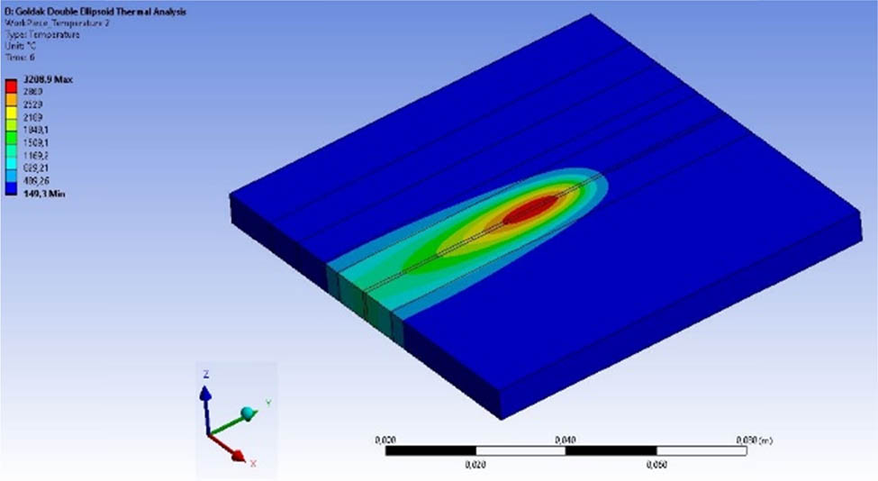
Temperature distribution at the top face after 6 s.

Temperature distribution at the top face after 10 s.
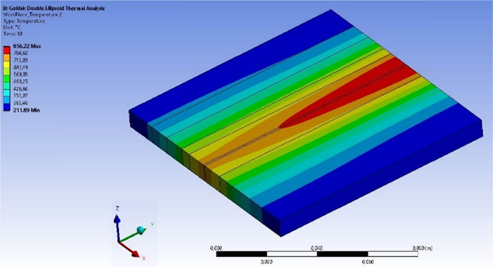
Temperature distribution at the top face after 30 s.
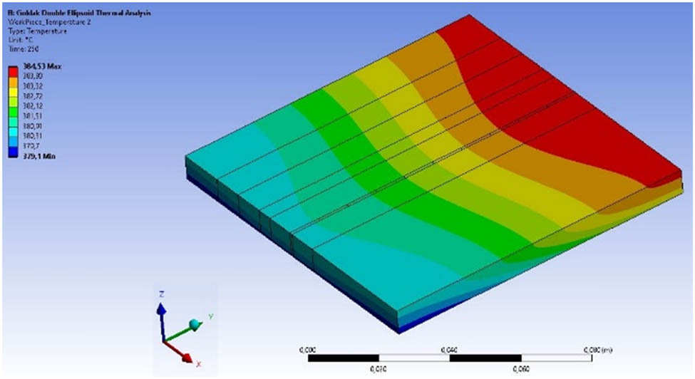
Temperature distribution at the top face after 250 s.
To investigate the temperature profile through the thickness of the workpiece, a midsection at the weldline was targeted. Figures 21–23 show the temperature distributions after 6, 10, and 250 s, respectively.
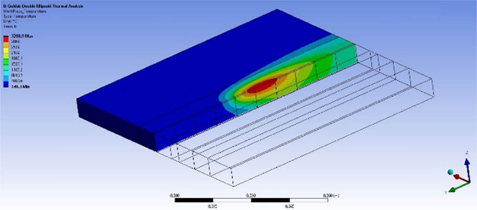
Temperature distribution at the middle of the weld line after 6 s.

Temperature distribution at the middle of the weld line after 10 s.
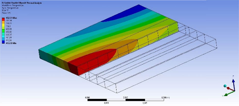
Temperature distribution at the middle of the weld line after 250 s.
Figures 24 and 25 depict the top and bottom faces of the welded specimen, respectively. The welding direction, the TC locations, and the welding parameters are indicated on the top face.

Top face of the welded specimen.

Bottom face of the welded specimen.
The sample part was preheated to approximately 150°C before welding. At the start of welding, the temperatures of TCs (TC1, TC2, TC3, TC4, and TC5) were recorded as 129.4, 158.7, 157.2, 139, and 153.1°C, respectively. Before the welding started, the heating apparatus was removed from the workpiece, which resulted in some temperature drops on the part.
Each TC value obtained from experiments was compared with the corresponding node temperature in FEM, as shown in separate graphs in Figures 27–31.
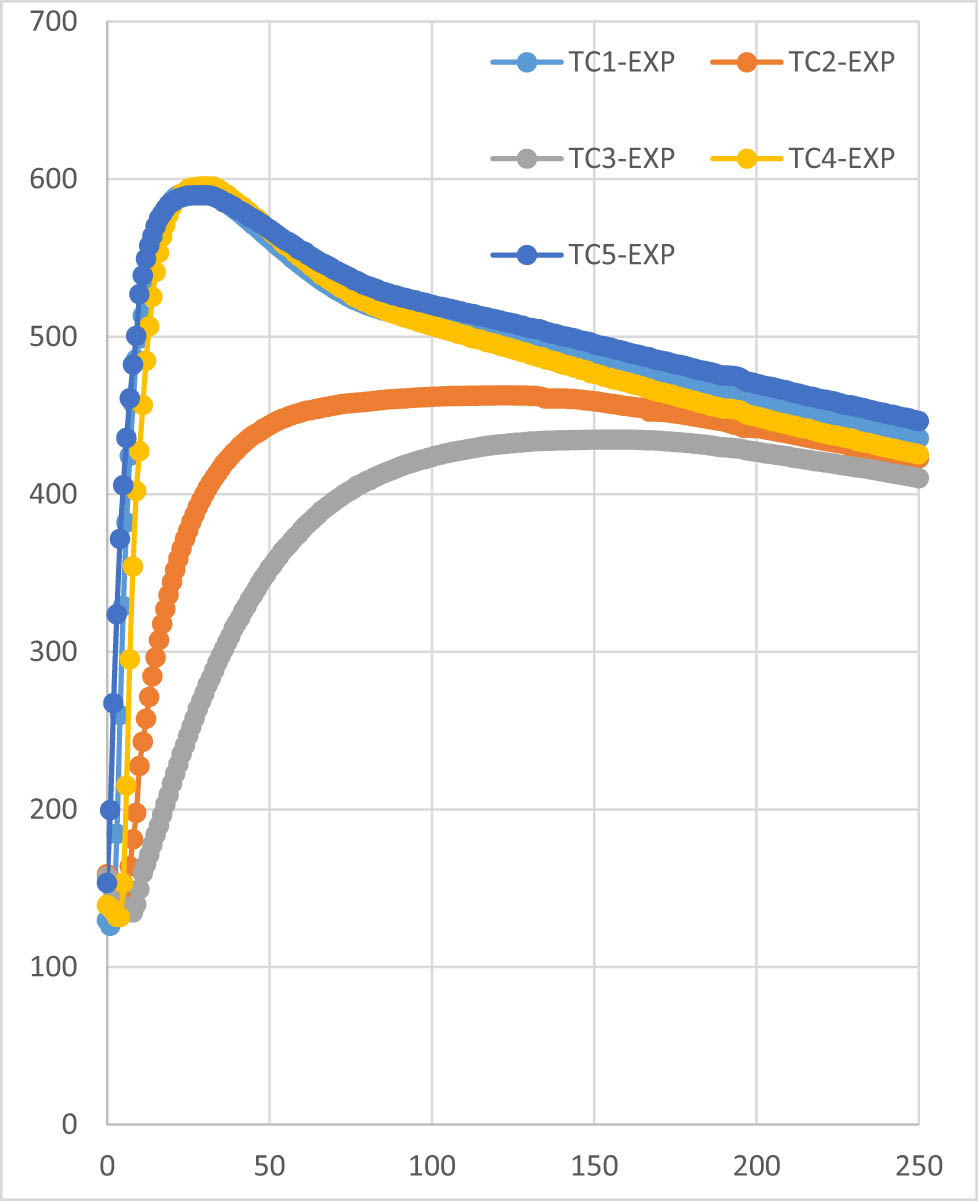
Experimental data for temperature (vertical) vs time (horizontal) graph for each TC point.

Numerical FEM data for temperature (vertical) vs time (horizontal) graph corresponding to each TC location.
Comparison of temperature vs time history for the experimental and the FEM results at TC1.

Comparison of temperature vs time history for the experimental and the FEM results at TC2.
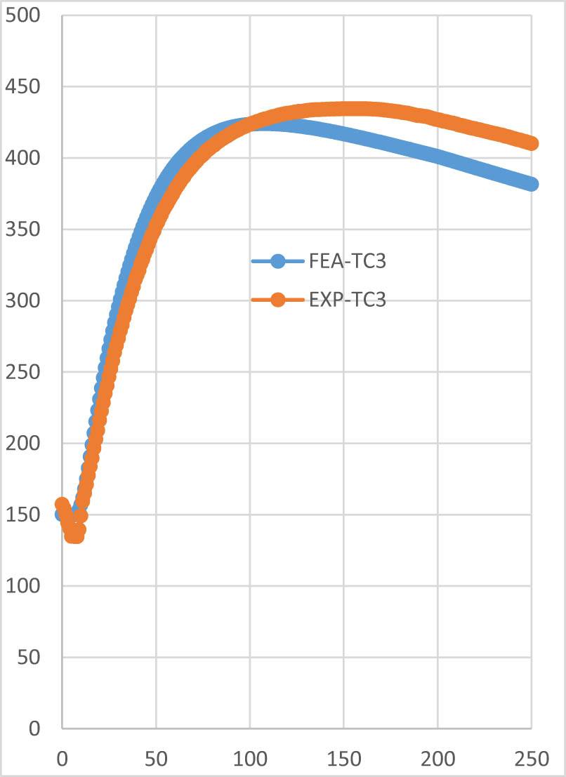
Comparison of temperature vs time history for the experimental and the FEM results at TC3.
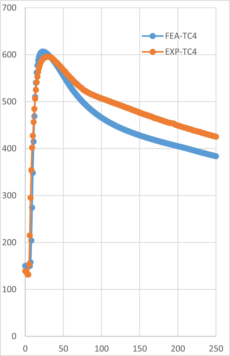
Comparison of temperature vs time history for the experimental and the FEM results at TC4.
The experimental and FE (FEM) results for temperature history belonging to each of the five-TC locations are shown in Figures 26 and 27, respectively.
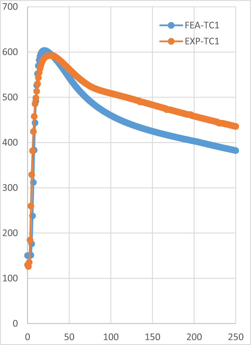
The temperature distribution recorded during the experimental work is compared with the results obtained from the FEA. Since a cumulative comparison graph involving ten curves (five for the experimental, and another five for the numerical results) would make the display cumbersome, individual comparisons are opted for each TC location. These comparisons are shown in Figures 28–32 for the TC points of TC1, TC2, TC3, TC4, and TC5, respectively. A strong correlation between the two sets of data is observed, confirming the capability of the numerical model in predicting temperature profiles during SAW of SA 387 Grade 11 Class 2 steel.
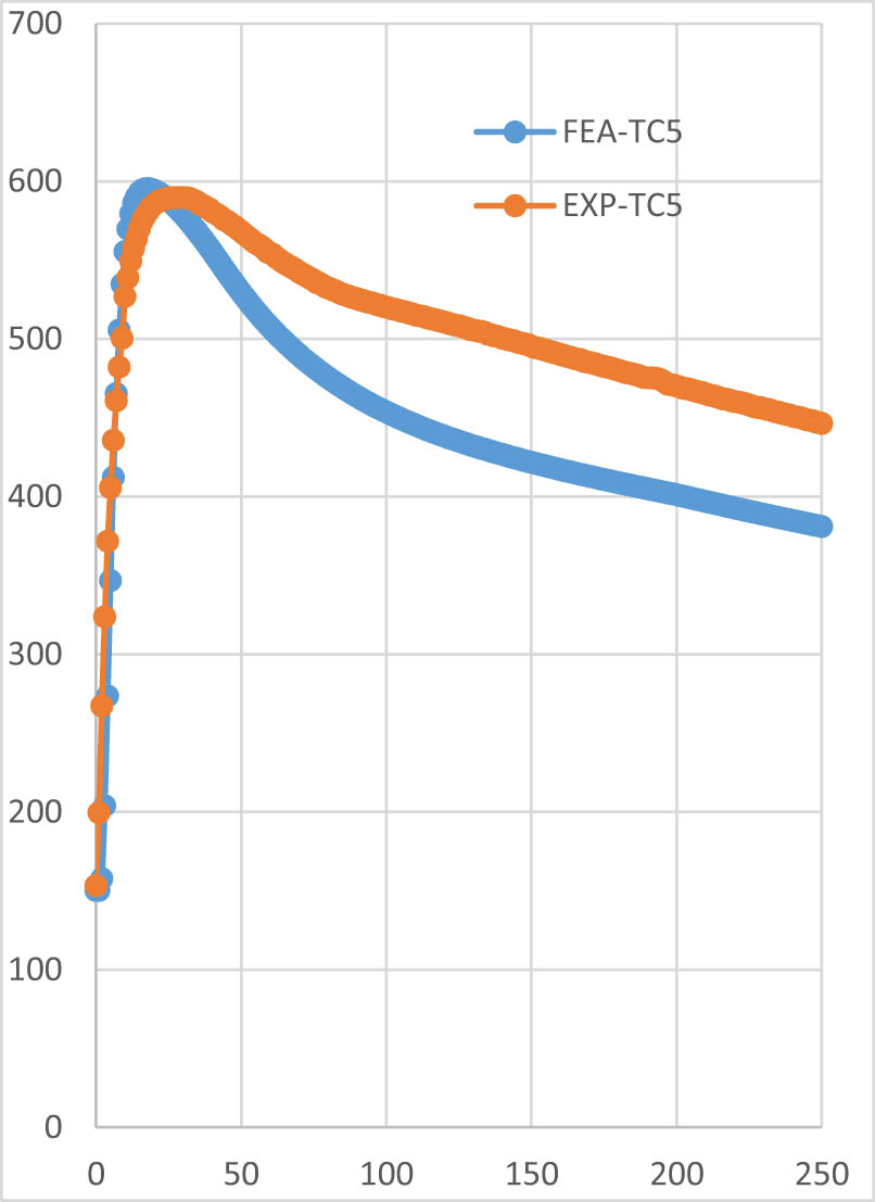
Comparison of temperature vs time history for the experimental and the FEM results at TC5.
Figures 26 and 27 illustrate the temperature variations over time for specific points. As the heat source approaches a point, its temperature increases, and as the heat source moves away, the temperature gradually decreases. Notably, at points 1, 4, and 5, located near the heat source, the temperatures are higher than those at points 2 and 3. Additionally, the temperature at point 2 is higher than that at point 3. Overall, a good agreement is observed between the predicted and experimental temperatures.
At point 1, as welding commenced, TC1 recorded a temperature of 129.4°C in the experimental work. The maximum temperature of 591.9°C was reached at 27 s, with the TC measuring the maximum value for the subsequent 4 s. According to the predicted temperature obtained from FEA at the node corresponding to TC1, the maximum temperature was 603.34°C at 20 s. This time difference is attributed to the response time of the recorder, which measures temperatures with a delay of 4–5 s. At 250 s, the temperature on the specimen was 435.3°C, while the predicted temperature by FEA was 382.17°C. Thus, for point 1, there is an observed difference of approximately 2% at the maximum temperature and approximately 13% at 250 s.
At point 2, when welding began, TC2 recorded a temperature of 158.7°C in the experimental work. The maximum temperature of 462.5°C was reached at 120 s, with the TC measuring the maximum value for the next 6 s. According to the predicted temperature obtained from FEA at the node corresponding to TC2, the maximum temperature was 452.43°C at 60 s. At 250 s, the temperature on the specimen was 422.6°C, while the predicted temperature by FEA was 381.8°C. Thus, for point 2, there is an observed difference of approximately 2% at the maximum temperature and approximately 10% at 250 s.
At point 3, when welding began, TC3 recorded a temperature of 157.2°C in the experimental work. The maximum temperature of 434.4°C was reached at 149 s, with the TC measuring the maximum value for the next 14 s. According to the predicted temperature obtained from FEA at the node corresponding to TC3, the maximum temperature was 423.94°C at 108 s. At 250 s, the temperature on the specimen was 410.0°C, while the predicted temperature by FEA was 381.49°C. Thus, for point 3, there is an observed difference of approximately 2.4% at the maximum temperature and approximately 7% at 250 s.
At point 4, when welding began, TC4 recorded a temperature of 139.0°C in the experimental work. The maximum temperature of 595.2°C was reached at 29 s, with the TC measuring the maximum value for the next 3 s. According to the predicted temperature obtained from FEA at the node corresponding to TC4, the maximum temperature was 606.58°C at 23 s. At 250 s, the temperature on the specimen was 425.1°C, while the predicted temperature by FEA was 400.09°C. Thus, for point 4, there is an observed difference of approximately 2% at the maximum temperature and approximately 10% at 250 s.
At point 5, when welding began, TC5 recorded a temperature of 153.1°C in the experimental work. The maximum temperature of 589.5°C was reached at 27 s, with the TC measuring the maximum value for the next 5 s. According to the predicted temperature obtained from FEA at the node corresponding to TC5, the maximum temperature was 599.25°C at 18 s. At 250 s, the temperature on the specimen was 446.2°C, while the predicted temperature by FEA was 380.89°C. Thus, for point 5, there is an observed difference of approximately 1% at the maximum temperature and approximately 15% at 250 s.
Table 9 exhibits the temperatures obtained from the experiments and the FE numerical solutions. It reveals inconsiderable deviations at the peak temperatures and minute differences at the end of the welding process.
Comparison of the experimental and the numerical FEM temperatures
| Points | FEM model | Experiment | Deviation at peak temp. (%) | Deviation at 250 s temp. (%) | ||||
|---|---|---|---|---|---|---|---|---|
| Peak temp. (°C) | Time (s) | Temp. at 250 s | Peak temp. (°C) | Time (s) | Temp. at 250 s | |||
| TC1 | 603.34 | 20 | 382.17 | 591.9 | 27 | 435.3 | 2 | 13 |
| TC2 | 452.43 | 60 | 381.8 | 462.5 | 108 | 422.6 | 2 | 10 |
| TC3 | 423.94 | 108 | 381.49 | 434.4 | 149 | 410.0 | 2.4 | 7 |
| TC4 | 606.58 | 23 | 400.9 | 595.2 | 29 | 425.1 | 2 | 10 |
| TC5 | 599.25 | 18 | 380.89 | 589.5 | 27 | 446.2 | 1 | 16 |
| Average | 1.88 | 11.2 | ||||||
Numerical FEA shows satisfactory results compared to experimental test results. Therefore, this model can be applied to predict thermal cycles for different welding parameters and materials. The effect of cooling rates on joint performance and residual stress determination can be investigated.
4 Conclusions
This study examines a comprehensive exploration of temperature distributions during SAW of SA 387-Gr.11-Cl.2 steel. We have successfully characterized the thermal behavior of SAW joints through a combination of meticulous experimental measurements and developed numerical FEA. For welding an 8 mm thick plate with one pass, the suitable parameters were found to be 600 A current, 31 V voltage, and 10 mm·s−1 welding speed. The development of an FEA model using ANSYS software incorporated 3D Goldak’s double ellipsoidal moving heat source model. The parameters for energy input were determined from the experiments and were incorporated into the model. Temperature profiles at specific points revealed a strong correlation between numerical predictions and experimental measurements. Any deviations between the two sets of data at maximum temperatures and the end of the welding process were thoroughly discussed. An average variation of 1.88% at peak temperatures and 11.8% at completion time was observed between the results. The experimental cooling periods were found to be slower than predicted by FEA. The results showed the temperature distribution at various time steps, illustrating the transient nature of the welding process. The findings demonstrate the accuracy of the numerical model in predicting temperature profiles during welding, providing valuable insights for understanding the HAZ, optimizing welding parameters, and controlling the microstructure and mechanical properties of welded structures. In addition to this, this work may be further extended by exploring the effect of cooling rates on joint performance and residual stresses.
Acknowledgements
This article is published in a preprint [38] that has not been peer-reviewed. The authors would like to extend their thanks to the reviewers of the manuscript for their valuable comments.
-
Funding information: The authors state no funding involved.
-
Author contributions: Murat Makaraci: conceptualization, methodology, validation, formal analysis, writing – review & editing, supervision. Mert Turgut Senol: methodology, validation, visualization, resources, investigation, formal analysis, experiments, writing.
-
Conflict of interest: The authors state no conflict of interest.
-
Data availability statement: The data that support the findings of this study are available from the corresponding author upon reasonable request.
References
[1] https://www.alloysteelplates.com/asme-sa-387-grade-11-class-2.html (Visit Date: 11 August 2022).Search in Google Scholar
[2] https://www.rextonsteel.com/sa-387-gr-11-cl-2-alloy-steel-plate-supplier-stockist.html (Visit Date: 11 August 2022).Search in Google Scholar
[3] Singh, R. Arc Welding processes handbook (First published), Scrivener Wiley, USA, 2021.10.1002/9781119819080Search in Google Scholar
[4] Mollicone, P., D. Camilleri, T. G. F. Gary, and T. Comlekci. Simple thermo-elastic-plastic models for welding distortion simulation. Journal of Materials Processing Technology, Vol. 176, No. 1–3, 2006, pp. 77–86.10.1016/j.jmatprotec.2006.02.022Search in Google Scholar
[5] Lindgren, L. E. Finite element modelling and simulation of welding. Part 1: increased complexity. Journal of Thermal Stresses, Vol. 24, No. 2, 2001, pp. 141–192.10.1080/01495730150500442Search in Google Scholar
[6] Lindgren, L. E. Finite element modelling and simulation of welding. Part 2: improved material modelling. Journal of Thermal Stresses, Vol. 24, No. 3, 2001, pp. 195–231.10.1080/014957301300006380Search in Google Scholar
[7] Lindgren, L. E. Finite element modelling and simulation of welding. Part 3: efficiency and integration. Journal of Thermal Stresses, Vol. 24, No. 4, 2001, pp. 305–334.10.1080/01495730151078117Search in Google Scholar
[8] Teng, T. L. , P. H. Chang, and W. C. Tseng. Effect of welding sequences on residual stresses. Computers and Structures, Vol. 81, No. 5, 2003, pp. 273–286.10.1016/S0045-7949(02)00447-9Search in Google Scholar
[9] Chang, P. H. and T. L. Teng. Numerical and experimental investigations on the residual stresses of the butt-welded joints. Computational Materials Science, Vol. 29, No. 4, 2004, pp. 511–522.10.1016/j.commatsci.2003.12.005Search in Google Scholar
[10] Armentani, E., R. Esposito, and R. Sepe. Finite element analysis of residual stresses on butt welded joints. Proceedings ESDA2006, Turin, Italy, 2006.10.1115/ESDA2006-95125Search in Google Scholar
[11] Armentani, E., R. Esposito, and R. Sepe. The effect of thermal properties and weld efficiency on residual stresses in welding. Journal of Achievements in Materials and Manufacturing Engineering, Vol. 20, 2007, pp. 319–322.Search in Google Scholar
[12] Armentani, E., R. Esposito, and R. Sepe. The influence of thermal properties and preheating on residual stresses in welding. International Journal of Computational Materials Science and Surface Engineering, Vol. 1, No. 2, 2007, pp. 146–162.10.1504/IJCMSSE.2007.014870Search in Google Scholar
[13] Armentani, E., E. Pozzi, and R. Sepe. Finite element simulation of temperature fields and residual stresses in butt welded joints and comparison with experimental measurements. Proceedings ESDA2014, Copenhagen, Denmark, 2014.10.1115/ESDA2014-20541Search in Google Scholar
[14] Kermanpur, A., M. Shamanian, and V. E. Yeganeh. Three-dimensional thermal simulation and experimental investigation of GTAW circumferentially butt-welded Incoloy 800 pipes. Journal of Materials Processing Technology, Vol. 199, No. 1–3, 2008, pp. 295–303.10.1016/j.jmatprotec.2007.08.009Search in Google Scholar
[15] Sepe, R., E. Armentani, G. Lamanna, and F. Caputo. Evaluation by FEM of the influence of the preheating and post-heating treatments on residual stresses in welding. Key Engineering Materials, Vol. 628, 2015, pp. 93–96.10.4028/www.scientific.net/KEM.627.93Search in Google Scholar
[16] Sepe, R., M. Laiso, A. De Luca, and F. Caputo. Evaluation of residual stresses in butt welded joint of dissimilar material by FEM. Key Engineering Materials, Vol. 754, 2017, pp. 268–271.10.4028/www.scientific.net/KEM.754.268Search in Google Scholar
[17] Mondal, A. K. , P. Biswas, and S. Bag. Prediction of welding sequence induced thermal history and residual stresses and their effect on welding distortion. Welding in the World, Vol. 61, No. 4, 2017, pp. 711–721.10.1007/s40194-017-0468-3Search in Google Scholar
[18] Hashemzadeh, M., B. Q. Chen, and C. G. Soares. Evaluation of multipass welding-induced residual stress using numerical and experimental approach. Ships Offshore Structure, Vol. 13, No. 8, 2018, pp. 847–856.10.1080/17445302.2018.1470453Search in Google Scholar
[19] Tsirkas, S. A. Numerical simulation of the laser welding process for the prediction of temperature distribution on welded aluminum aircraft components. Optics & Laser Technology, Vol. 100, 2018, pp. 45–56.10.1016/j.optlastec.2017.09.046Search in Google Scholar
[20] Ferro, P., F. Berto, and M. N. James. A simplified model for TIG dressing numerical simulation. Modelling and Simulation in Materials Science and Engineering, Vol. 25, No. 3, 2017, pp. 1–16.10.1088/1361-651X/aa623dSearch in Google Scholar
[21] Ferro, P., F. Bonollo, F. Berto, and A. Montanari. Numerical modeling of residual stress redistribution induced by TIG-dressing. Frattura ed Integrità Strutturale, Vol. 47, 2019, pp. 221–230.10.3221/IGF-ESIS.47.17Search in Google Scholar
[22] Choi, J. and J. Mazumder. Numerical and experimental analysis for solidification and residual stress in the GMAW process for AISI 304 stainless steel. Journal of Materials Science, Vol. 37, No. 10, 2002, pp. 2143–2158.10.1023/A:1015258322780Search in Google Scholar
[23] Tsirkas, S. A. , P. Papanikos, and T. Kermanidis. Numerical simulation of the laser welding process in butt-joint specimens. Journal of Materials Processing Technology, Vol. 134, No. 1, 2003, pp. 59–69.10.1016/S0924-0136(02)00921-4Search in Google Scholar
[24] Cho, J. R. , B. Y. Lee, Y. H. Moon, and C. J. Van Tyne. Investigation of residual stress and post-weld heat treatment of multi-pass welds by finite element method and experiments. Journal of Materials Processing Technology, Vol. 1695, 2004, pp. 155-156.10.1016/j.jmatprotec.2004.04.325Search in Google Scholar
[25] Gery, D., H. Long, and P. Maropoulos. Effects of welding speed, energy input and heat source distribution on temperature variations in butt joint welding. Journal of Materials Processing Technology, Vol. 167, No. 2–3, 2005, pp. 393–401.10.1016/j.jmatprotec.2005.06.018Search in Google Scholar
[26] Citarella, R., P. Carlone, M. Lepore, and R. Sepe. Hybrid technique to assess the fatigue performance of multiple cracked FSW joints. Engineering Fracture Mechanics, Vol. 162, 2016, pp. 38–50.10.1016/j.engfracmech.2016.05.005Search in Google Scholar
[27] Citarella, R., P. Carlone, R. Sepe, and M. Lepore. DBEM crack propagation in friction stir welded aluminum joints. Advances in Engineering Software, Vol. 101, 2016, pp. 50–59.10.1016/j.advengsoft.2015.12.002Search in Google Scholar
[28] Mochizuki, M., M. Hayashi, and T. Hattori. Numerical analysis of welding residual stress and its verification using neutron diffraction measurement. Transaction ASME, Vol. 122, 2000, pp. 98–103.10.1115/1.482772Search in Google Scholar
[29] Yadav, G. P. K., D. Bandhu, B. Y. Krishna, N. Gupta, P. Jha, J. J. Vora, et al. Exploring the potential of metal-cored filler wire in gas metal arc welding for ASME SA387-Gr.11-Cl.2 steel joints. Journal of Adhesion Science and Technology, Vol. 38, No. 2, 2024, pp. 163–184.10.1080/01694243.2023.2223367Search in Google Scholar
[30] Bandhu, D., E. V. Goud, J. J. Vora, S. Das, K. Abhishek, R. K. Gupta, et al. Influence of regulated metal deposition and gas metal arc welding on ASTM A387-11–2 steel plates: as-deposited inspection, microstructure, and mechanical properties. Journal of Materials Engineering and Performance, Vol. 32, 2023, pp. 1025–1038.10.1007/s11665-022-07185-6Search in Google Scholar
[31] Bandhu, D., J. J. Vora, S. Das, A. Thakur, S. Kumari, K. Abhishek, et al. Experimental study on application of gas metal arc welding based regulated metal deposition technique for low alloy steel. Materials and Manufacturing Processes, Vol. 37, No. 15, 2022, pp. 1727–1745.10.1080/10426914.2022.2049298Search in Google Scholar
[32] Bandhu, D., F. Djavanroodi, G. Shaikshavali, J. J. Vora, K. Abhishek, A. Thakur, et al. Effect of metal-cored filler wire on surface morphology and micro-hardness of regulated metal deposition welded ASTM A387-Gr.11-Cl.2 steel plates. Materials, Vol. 15, 2022, id. 6661.10.3390/ma15196661Search in Google Scholar PubMed PubMed Central
[33] Bandhu, D. and K. Abhishek. Assessment of weld bead geometry in modified shortcircuiting gas metal arc welding process for low alloy steel. Materials and Manufacturing Processes, Vol. 36, No. 12, 2021, pp. 1384–1402.10.1080/10426914.2021.1906897Search in Google Scholar
[34] Bandhu, D., S. Kumari, V. Prajapati, K. K. Saxena, and K. Abhishek. Experimental investigation and optimization of RMDTM welding parameters for ASTM A387 grade 11 steel. Materials and Manufacturing Processes, Vol. 36, No. 13, 2021, pp. 1524–1534.10.1080/10426914.2020.1854472Search in Google Scholar
[35] Bandhu, D., V. Prajapati, J. J. Vora, S. Das, K. Abhishek. Experimental studies of regulated metal deposition (RMD™) on ASTM A387 (11) steel: study of parametric influence and welding performance optimization. Journal of the Brazilian Society of Mechanical Sciences and Engineering, Vol. 42, 2020, id. 78.10.1007/s40430-019-2155-3Search in Google Scholar
[36] Sepe, R., A. D. Luca, A. Greco, and E. Armentani. Numerical evaluation of temperature fields and residual stresses in butt weld joints and comparison with experimental measurements. Fatigue & Fracture of Engineering Materials & Structures, Vol. 44, No. 1, 2020, pp. 182–198.10.1111/ffe.13351Search in Google Scholar
[37] American Petroleum Institute, API RP 934-C, Standart, 2nd Edition, February 2019, Materials and Fabrication of 11/4Cr-1/2Mo Steel Heavy Wall Pressure Vessels for High-pressure Hydrogen Service Operating at or Below 825 °F (440°C).Search in Google Scholar
[38] Suman, S. and P. Biswas. Comparative study on SAW welding induced distortion and residual stresses of CSEF steel considering solid state phase transformation and preheating. Journal of Manufacturing Processes, Vol. 51, 2020, pp. 19–30.10.1016/j.jmapro.2020.01.012Search in Google Scholar
[39] Makaracı, M., and M. T. Şenol. Transient temperature distribution estimation in submerged arc welding process applied To A387 chromium-molybdenum alloy steel using goldak’s double ellipsoidal moving heat source model. In Proceedings International Azerbaijan Academic Research Congress, Baku, Azerbaijan, 2022, pp. 325–336, 2022 ISBN: 978-605-71461-7-5.Search in Google Scholar
[40] Ghosh, A., N. Barman, H. Chattopadhyay, and S. Bag. Modelling of heat transfer in submerged arc welding process. Journal of Engineering Manufacture, Vol. 227, No. 10, 2013, pp. 1467–1473.10.1177/0954405413489291Search in Google Scholar
[41] The American Society of Mechanical Engineers ASME. ASME boiler and pressure vessel code section II, materials. ASME BPVC.II. D. M.-2021, New York, USA, 2021.Search in Google Scholar
[42] Kumar, S. K. Thermal field and residual stress analyses of GTAW dissimilar weldments between AA 5052 and AA 7075 by numerical simulation and experimentation, Master Thesis. CMR Institute of Technology, Department of Mechanical Engineering, 2020.Search in Google Scholar
[43] Taskaya, S., A. K. Gur, and C. Ozay. Joining of ramor 500 steel with SAW (submerged arc welding) and its evaluation of thermomechanical analysis in ANSYS package software. Thermal Science and Engineering Progress, Vol. 13, No. 2019, 2019, id. 100396.10.1016/j.tsep.2019.100396Search in Google Scholar
[44] Nart, E. and Y. Celik. A practical approach for simulating submerged arc welding process using FE Method. Journal of Constructional Steel Research, Vol. 84, No. 62–71, 2013, id. 2013.10.1016/j.jcsr.2013.02.005Search in Google Scholar
[45] Goldak, J., A. Chakravarti, and M. Bibby. A new finite model for welding heat sources. Metallurgical Transactions B, Vol. 15B, 1984 June, pp. 299–305.10.1007/BF02667333Search in Google Scholar
[46] Biswas, P. and A. K. Mondal. A comparative study of three different approaches of FE analysis for prediction of welding distortion of orthogonally stiffened plate panels. Journal of Ship Production and Design, Vol. 25, No. 4, 2009, pp. 1–7.10.5957/jsp.2009.25.4.191Search in Google Scholar
[47] Makaraci, M. and M. T. Senol. Numerical and experimental investigation of temperature distribution in submerged Arc welding of high-temperature resistant anti-corrosive pressure vessel steel SA 387. Authorea, Vol. 1, 2023, pp. 1–29.10.22541/au.169581658.89623547/v1Search in Google Scholar
© 2024 the author(s), published by De Gruyter
This work is licensed under the Creative Commons Attribution 4.0 International License.
Articles in the same Issue
- Research Articles
- De-chlorination of poly(vinyl) chloride using Fe2O3 and the improvement of chlorine fixing ratio in FeCl2 by SiO2 addition
- Reductive behavior of nickel and iron metallization in magnesian siliceous nickel laterite ores under the action of sulfur-bearing natural gas
- Study on properties of CaF2–CaO–Al2O3–MgO–B2O3 electroslag remelting slag for rack plate steel
- The origin of {113}<361> grains and their impact on secondary recrystallization in producing ultra-thin grain-oriented electrical steel
- Channel parameter optimization of one-strand slab induction heating tundish with double channels
- Effect of rare-earth Ce on the texture of non-oriented silicon steels
- Performance optimization of PERC solar cells based on laser ablation forming local contact on the rear
- Effect of ladle-lining materials on inclusion evolution in Al-killed steel during LF refining
- Analysis of metallurgical defects in enamel steel castings
- Effect of cooling rate and Nb synergistic strengthening on microstructure and mechanical properties of high-strength rebar
- Effect of grain size on fatigue strength of 304 stainless steel
- Analysis and control of surface cracks in a B-bearing continuous casting blooms
- Application of laser surface detection technology in blast furnace gas flow control and optimization
- Preparation of MoO3 powder by hydrothermal method
- The comparative study of Ti-bearing oxides introduced by different methods
- Application of MgO/ZrO2 coating on 309 stainless steel to increase resistance to corrosion at high temperatures and oxidation by an electrochemical method
- Effect of applying a full oxygen blast furnace on carbon emissions based on a carbon metabolism calculation model
- Characterization of low-damage cutting of alfalfa stalks by self-sharpening cutters made of gradient materials
- Thermo-mechanical effects and microstructural evolution-coupled numerical simulation on the hot forming processes of superalloy turbine disk
- Endpoint prediction of BOF steelmaking based on state-of-the-art machine learning and deep learning algorithms
- Effect of calcium treatment on inclusions in 38CrMoAl high aluminum steel
- Effect of isothermal transformation temperature on the microstructure, precipitation behavior, and mechanical properties of anti-seismic rebar
- Evolution of residual stress and microstructure of 2205 duplex stainless steel welded joints during different post-weld heat treatment
- Effect of heating process on the corrosion resistance of zinc iron alloy coatings
- BOF steelmaking endpoint carbon content and temperature soft sensor model based on supervised weighted local structure preserving projection
- Innovative approaches to enhancing crack repair: Performance optimization of biopolymer-infused CXT
- Structural and electrochromic property control of WO3 films through fine-tuning of film-forming parameters
- Influence of non-linear thermal radiation on the dynamics of homogeneous and heterogeneous chemical reactions between the cone and the disk
- Thermodynamic modeling of stacking fault energy in Fe–Mn–C austenitic steels
- Research on the influence of cemented carbide micro-textured structure on tribological properties
- Performance evaluation of fly ash-lime-gypsum-quarry dust (FALGQ) bricks for sustainable construction
- First-principles study on the interfacial interactions between h-BN and Si3N4
- Analysis of carbon emission reduction capacity of hydrogen-rich oxygen blast furnace based on renewable energy hydrogen production
- Just-in-time updated DBN BOF steel-making soft sensor model based on dense connectivity of key features
- Effect of tempering temperature on the microstructure and mechanical properties of Q125 shale gas casing steel
- Review Articles
- A review of emerging trends in Laves phase research: Bibliometric analysis and visualization
- Effect of bottom stirring on bath mixing and transfer behavior during scrap melting in BOF steelmaking: A review
- High-temperature antioxidant silicate coating of low-density Nb–Ti–Al alloy: A review
- Communications
- Experimental investigation on the deterioration of the physical and mechanical properties of autoclaved aerated concrete at elevated temperatures
- Damage evaluation of the austenitic heat-resistance steel subjected to creep by using Kikuchi pattern parameters
- Topical Issue on Focus of Hot Deformation of Metaland High Entropy Alloys - Part II
- Synthesis of aluminium (Al) and alumina (Al2O3)-based graded material by gravity casting
- Experimental investigation into machining performance of magnesium alloy AZ91D under dry, minimum quantity lubrication, and nano minimum quantity lubrication environments
- Numerical simulation of temperature distribution and residual stress in TIG welding of stainless-steel single-pass flange butt joint using finite element analysis
- Special Issue on A Deep Dive into Machining and Welding Advancements - Part I
- Electro-thermal performance evaluation of a prismatic battery pack for an electric vehicle
- Experimental analysis and optimization of machining parameters for Nitinol alloy: A Taguchi and multi-attribute decision-making approach
- Experimental and numerical analysis of temperature distributions in SA 387 pressure vessel steel during submerged arc welding
- Optimization of process parameters in plasma arc cutting of commercial-grade aluminium plate
- Multi-response optimization of friction stir welding using fuzzy-grey system
- Mechanical and micro-structural studies of pulsed and constant current TIG weldments of super duplex stainless steels and Austenitic stainless steels
- Stretch-forming characteristics of austenitic material stainless steel 304 at hot working temperatures
- Work hardening and X-ray diffraction studies on ASS 304 at high temperatures
- Study of phase equilibrium of refractory high-entropy alloys using the atomic size difference concept for turbine blade applications
- A novel intelligent tool wear monitoring system in ball end milling of Ti6Al4V alloy using artificial neural network
- A hybrid approach for the machinability analysis of Incoloy 825 using the entropy-MOORA method
- Special Issue on Recent Developments in 3D Printed Carbon Materials - Part II
- Innovations for sustainable chemical manufacturing and waste minimization through green production practices
- Topical Issue on Conference on Materials, Manufacturing Processes and Devices - Part I
- Characterization of Co–Ni–TiO2 coatings prepared by combined sol-enhanced and pulse current electrodeposition methods
- Hot deformation behaviors and microstructure characteristics of Cr–Mo–Ni–V steel with a banded structure
- Effects of normalizing and tempering temperature on the bainite microstructure and properties of low alloy fire-resistant steel bars
- Dynamic evolution of residual stress upon manufacturing Al-based diesel engine diaphragm
- Study on impact resistance of steel fiber reinforced concrete after exposure to fire
- Bonding behaviour between steel fibre and concrete matrix after experiencing elevated temperature at various loading rates
- Diffusion law of sulfate ions in coral aggregate seawater concrete in the marine environment
- Microstructure evolution and grain refinement mechanism of 316LN steel
- Investigation of the interface and physical properties of a Kovar alloy/Cu composite wire processed by multi-pass drawing
- The investigation of peritectic solidification of high nitrogen stainless steels by in-situ observation
- Microstructure and mechanical properties of submerged arc welded medium-thickness Q690qE high-strength steel plate joints
- Experimental study on the effect of the riveting process on the bending resistance of beams composed of galvanized Q235 steel
- Density functional theory study of Mg–Ho intermetallic phases
- Investigation of electrical properties and PTCR effect in double-donor doping BaTiO3 lead-free ceramics
- Special Issue on Thermal Management and Heat Transfer
- On the thermal performance of a three-dimensional cross-ternary hybrid nanofluid over a wedge using a Bayesian regularization neural network approach
- Time dependent model to analyze the magnetic refrigeration performance of gadolinium near the room temperature
- Heat transfer characteristics in a non-Newtonian (Williamson) hybrid nanofluid with Hall and convective boundary effects
- Computational role of homogeneous–heterogeneous chemical reactions and a mixed convective ternary hybrid nanofluid in a vertical porous microchannel
- Thermal conductivity evaluation of magnetized non-Newtonian nanofluid and dusty particles with thermal radiation