Spatiotemporal water quality analysis of Vrana Lake, Croatia
-
Anja Batina
 ,
Neven Cukrov
,
Neven Cukrov

Abstract
The comprehensive analysis of spatiotemporal variations in water quality is crucial for ecosystem management. This study analyses and maps spatiotemporal variations in water quality at Vrana Lake, a coastal shallow lake in Dalmatia, Croatia. We established a monitoring grid of 20 stations and conducted monthly in situ measurements of seven water quality parameters from July 2023 to June 2024 using multiparameter probe. We measured electrical conductivity, turbidity, salinity, water temperature, dissolved oxygen, oxygen saturation, and chlorophyll-a. We analysed the correlation between these parameters, water level, and meteorological factors over a year and the impact of climate change over the 34 years. Additionally, we evaluated 15 geographic information system (GIS) spatial interpolation methods for mapping the distribution of water quality parameters, using root mean square error (RMSE) and mean error (ME) metrics. The vertical stratification analysis revealed that the lake’s shallow nature allows effective assessment through median values. Key findings highlighted that air temperature, precipitation, and wind significantly affect water quality dynamics. The Simple Kriging – Trend emerged as the best GIS spatial interpolation method for modelling water quality parameters. Overall, this study enhances the understanding of water quality variations and their implications for ecosystem health in coastal shallow lakes.
Graphical abstract
Abbreviations
- AP
-
air pressure
- AT
-
air temperature
- Chl-a
-
chlorophyll-a
- DO
-
dissolved oxygen
- EBK
-
Empirical Bayesian Kriging
- EC
-
electrical conductivity
- GIS
-
geographic information system
- MAD
-
median absolute deviation
- MASL
-
meters above sea level
- ME
-
mean error
- PP
-
precipitation
- RH
-
relative humidity
- RMSE
-
root mean square error
- SH
-
sunshine hours
- SK
-
Simple Kriging
- SO
-
oxygen saturation
- WL
-
water level
- WS
-
wind speed
- WT
-
water temperature
1 Introduction
Water quality monitoring is a vital segment of effective management and preservation of water ecosystems [1], particularly in the context of climate change threats to lake ecosystems [2]. The intergovernmental panel on climate change (IPCC) [3] anticipates that rising global temperatures and extreme weather events, such as heavy precipitation, will affect coastal ecosystems and increase local flooding. Climatic factors, such as precipitation (PP), air temperature (AT), wind speed (WS), and sunshine hours (SH), are expected to significantly influence lake water quality [4], with warmer temperatures and heavy rainfall contributing to nutrient release and pollution [5]. The ongoing issue of eutrophication in lakes has prompted extensive research into the interplay between climate change and water quality [4,5,6].
Numerous models and methods have been developed to evaluate spatial and seasonal variations in water quality parameters. Commonly used methods include water quality index [7,8,9] and tropic state index [5], alongside multivariate statistical analysis like principal components analysis [10] and cluster analysis [11]. Moreover, advancements in data mining [12] and machine learning methods [4,13] have proven effective in modelling water quality parameters and identifying pollution sources. Utilizing spatial data science and geographic information system (GIS) is essential for addressing pressing issues such as climate change, as geospatial methods play a crucial role in comprehending complex environmental challenges and monitoring [14,15].
The need for a robust and optimized monitoring network is emphasized to monitor water quality trends and inform environmental management strategies [10,11,16]. Recent studies also highlight the significance of understanding vertical variability in water quality parameters, which can be influenced by factors such as nutrients level, light penetration, and temperature gradients within lakes [1,17,18].
GIS-based spatial interpolation methods are used to estimate water quality parameters in locations lacking direct measurements. Frequently used methods are inverse distance weighted [19,20], universal Kriging, and ordinary Kriging methods [21,22]. In addition to water quality studies, GIS software has been extensively applied in broader geographic analyses. For instance, Vujović et al. [23] used ArcGIS and QGIS to analyse geomorphometry in the Ibar River basin, while Oseke et al. [24] applied GIS and a water quality index to assess reservoirs affected by water diversion. Aleksova et al. [25] modelled erosion and mass movements in North Macedonia using GIS-based multi-hazard assessments, and Durlević [26] evaluated flood and landslide susceptibility in Serbia’s Mlava River Basin using similar tools. Recent studies have focused on comparison between different GIS spatial interpolation methods for groundwater levels [27] and sediment distribution in coastal areas [28]. However, there is a lack of studies comprehensively evaluating the effectiveness of different GIS spatial interpolation methods specifically for lake water quality assessment. The study by Ouabo et al. [29] emphasizes the importance of selecting suitable interpolation methods, particularly considering the non-normal distribution of water quality parameters, to avoid biased results [30].
This study is part of a broader research initiative aimed at enhancing lake water quality monitoring and assessment through the integration of in situ measurements, GIS multicriteria analysis, satellite imagery, and machine learning. In the initial phase of the research initiative, Batina and Krtalić [31] established a comprehensive framework that includes a theoretical analysis of lake dynamics, operational data collection, and spatiotemporal distribution analysis. Building on that work, in this study, we aimed to investigate the seasonal and spatial variations in water quality parameters in Vrana Lake in Dalmatia, Croatia, where eutrophication issues, exacerbated by nutrient influx, have led to phytoplankton and cyanobacteria growth, causing the extinction of macrophytes [32]. A study by Trbojević et al. [33] indicates macrophytes absence in 2020 and 2021 in the lake, with chlorophyll-a (Chl-a) concentration serving as a key indicator of this ecological change [2].
In this study, we aim to investigate the seasonal and spatial variability of water quality parameters in Vrana Lake, Croatia, and to analyse their correlation with water level (WL) and meteorological factors over a 12-month monitoring period. Additionally, we assess the long-term impact of climate change on the lake ecosystem using 34 years of historical WL and meteorological data spanning from 1990 to 2023. A key objective is to evaluate and identify the most suitable GIS spatial interpolation method for accurately mapping the distribution of water quality parameters. This research is significant for advancing lake monitoring practices, supporting adaptive management strategies in response to climate change, and providing a foundation for future studies utilizing GIS multicriteria analysis, remote sensing, and machine learning.
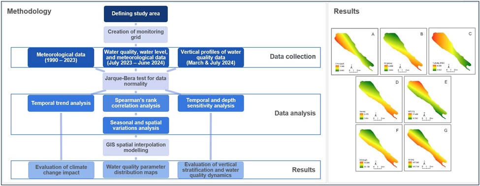
2 Methods
2.1 Study area and monitoring
Vrana Lake, located in Dalmatia near the eastern Adriatic coastline, is the largest natural lake in Croatia (Figure 1a), covering an area of approximately 30 km2 [34], and is situated between 43°51′–43°57′N latitude and 15°30′–15°39′E longitude (WGS84 coordinate system). Its ecological characteristics and biodiversity have led to its protection as a nature park. The lake is characterized by shallow water that fluctuates seasonally, with higher levels in winter and spring (highest mean WL was 1.28 m above sea level (MASL) from 1990 to 2023) and lower levels in summer and autumn (lowest mean WL was 0.41 MASL from 1990 to 2023), based on data provided by the Croatian Meteorological and Hydrological Service (DHMZ) and visualized in Figure 2. The lake’s shallowness and geolocation make it particularly susceptible to wind influences that promote water column mixing [35]. In May 2023, heavy rainfall resulted in unusually high WL in subsequent months (Figure 2), highlighting the importance of considering meteorological and WL data in understanding water quality [36].
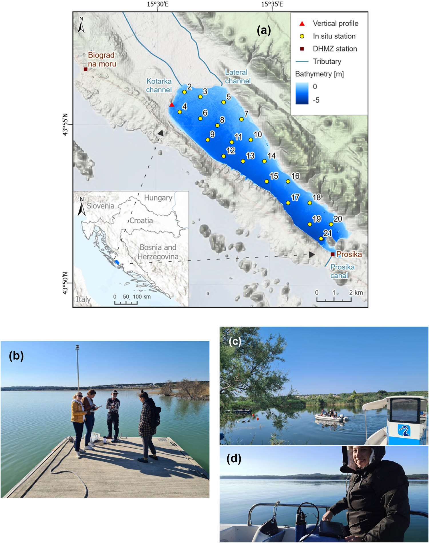
An overview of (a) Vrana Lake position and in situ stations, (b) preparation for measuring vertical profiles, and (c) and (d) in situ monitoring.
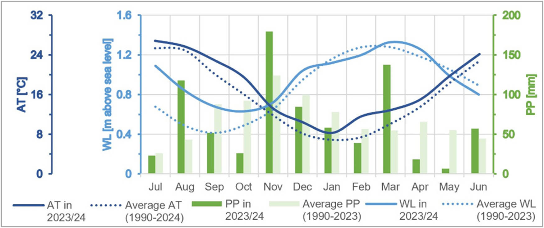
Comparison of AT, PP, and WL data for the research period of 2023/24 against historical averages.
Several factors contribute to the WL dynamics of Vrana Lake, including its connections to the Adriatic Sea, freshwater tributaries, brackish submerged groundwater discharge in the lake, underground karst fissures, and evaporation. During periods when WL drops below sea level, the lake’s salinity increases significantly due to the seawater influx through the artificial Prosika canal (Figure 1a). Additionally, the lake is affected by underground karst fissures along its western edge and the Jugovir brackish submerged groundwater discharge in the southern part, especially during strong south winds and high tides [37]. On the other hand, freshwater from surrounding karst fields and springs enters the lake through the Kotarka channel and the Lateral channel in the northern part (Figure 1a). Rainwater runoff from the northern and eastern hills is another significant source of water [32].
2.2 Data collection
In this study, we developed a comprehensive monitoring grid of 20 in situ stations for monthly in situ measurements of seven water quality parameters, including electrical conductivity (EC), turbidity, salinity, water temperature (WT), dissolved oxygen (DO), oxygen saturation (SO), and Chl-a, from July 2023 to June 2024 [38]. Furthermore, we analysed correlations between these parameters, WL, and six meteorological factors, such as AT, WS, PP, SH, relative humidity (RH), and atmospheric pressure (AP), in a 12-month period to understand their influence on lake ecosystem health. Additionally, we built upon the work of Rubinić and Katalinić [39] by analysing 34 years of WL and meteorological data (1990–2023), including AT and PP, to evaluate the more recent impact of climate change on the lake. Finally, we evaluated 15 GIS spatial interpolation methods to determine the best method for mapping water quality parameters, using cross-validation, root mean square error (RMSE), and mean error (ME). The flowchart is shown in Figure 3.
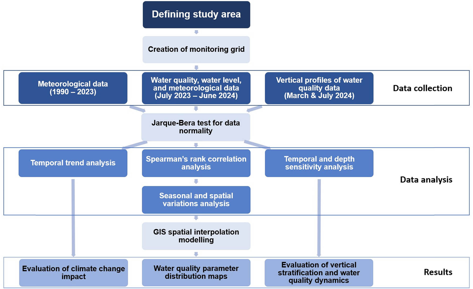
Flowchart illustrating the study’s methodology.
The lake’s ecological health is further impacted by anthropogenic influence from its tributaries [40] and influx of seawater via the Prosika canal, particularly during low WLs. To address these ecological concerns, we developed a new comprehensive monitoring grid designed to provide sufficient data for remote sensing and machine learning applications in subsequent research. Previously, monitoring efforts were limited to one station by the Water Institute Josip Juraj Strossmayer and three stations by the Public Institution Vransko Jezero Nature Park. We incorporated these existing stations and added new ones to ensure comprehensive spatial coverage. The 20 monitoring stations were strategically positioned (Figure 1a), considering lake’s characteristics, existing monitoring stations, the time required to complete the measurements by a vessel, and the hydrological model, including the lake’s bathymetry, tributaries, and connection to the sea [8].
We delineated the lake boundary using PlanetScope satellite imagery [41] and the Normalized Difference Water Index [42], focusing on the month of October 2023, when the WL was at its lowest during our year-long research period (Figure 2).
DHMZ provided historical monthly data on average AT and total PP from 1990 to 2023 for the Biograd na Moru station (43°56′44.5″N, 15°26′52.8″E, WGS84), along with average WL data from the Prosika station (43°51′0.3″N, 15°37′45.3″E, WGS84) (Figure 1a, Table S1). Additionally, they supplied daily meteorological data from the Biograd na Moru and Zadar stations, as well as WL data from the Prosika station, for our research period from July 2023 to June 2024 (Table 1 and Table S2). We analysed meteorological and WL parameters for each measurement day, except for PP, which we assessed based on the amount from 3 days prior. We adopted this methodology because we aimed to conduct in situ measurements on sunny, non-cloudy days, and we plan to integrate satellite data for specific measurement dates in our future research.
Summary of the dataset and probe specifications
| Type | Parameter | Abbreviation | Unit | YSI EXO2 [44] | |
|---|---|---|---|---|---|
| Range | Accuracy | ||||
| Water quality parameters | Chlorophyll-a | Chl-a | μg/L | 0–400 μg/L | — |
| Electrical conductivity | EC | dS/m | 0–100 dS/m | ±0.5% of reading or 0.001 dS/m | |
| Turbidity | — | FNU | 0–999 FNU | 0.3 FNU or ±2% of reading | |
| Salinity | — | — | 0–42 | ±0.1 | |
| Water temperature | WT | °C | −5 to 35°C | ±0.01°C | |
| Dissolved oxygen | DO | mg/L | 0–20 mg/L | ±1% of reading or 0.1 mg/L | |
| Oxygen saturation | SO | % | 0–200% | ±1% of reading or 1% air sat. | |
| Meteorological station | |||||
| Meteorological parameters | Air temperature | AT | °C | Biograd na Moru | |
| Wind speed | WS | Beaufort number | Biograd na Moru | ||
| Relative humidity | RH | % | Biograd na Moru | ||
| Atmospheric pressure | AP | hPa | Zadar | ||
| Amount of precipitation | PP | mm | Biograd na Moru | ||
| Sunshine hours | SH | h | Zadar | ||
| — | Water level | WL | m | Prosika | |
Researchers from Ruđer Bošković Institute collected in situ data on seven physicochemical and biological parameters in the lake (Table 1). Using the YSI EXO2 (YSI, USA) multiparameter probe, the team collected vertical profiles on a monthly basis from July 2023 to June 2024 (Figure 1c and d). These measurements were conducted between 8:00 and 13:00 at 20 designated monitoring stations (Table S3). Salinity is determined automatically from the sonde conductivity and temperature readings according to algorithms found in Standard Methods for the Examination of Water and Wastewater [43]. The use of the practical salinity scale results in values that are unitless, since the measurements are carried out in reference to the conductivity of standard water at 15°C [44]. Optical sensors in probes are increasingly important for real-time water quality assessment in environmental applications [45]. Due to poor weather conditions, we had to postpone our fieldwork scheduled for November 2023 to December 4th, and we conducted the December survey on the 19th, while all other measurements were conducted in their respective months.
2.3 Data analysis
2.3.1 Analysis of meteorological and water quality parameters
We used the Jarque–Bera test to assess the normality of historical monthly meteorological data, as well as meteorological and WL data for the research period [11]. The test evaluates whether sample data exhibit skewness and kurtosis consistent with a normal distribution, with p-values interpreted against a significance threshold of 0.05. For variables that did not meet the normality assumption, a cube root transformation was applied in Excel to normalize the data.
Furthermore, we used the Jarque–Bera test to assess the normality of raw water quality parameters such as Chl-a, EC, turbidity, salinity, WT, DO, and SO [11]. To address deviations from normality, we applied logarithmic, square root, cube root, and Box-Cox transformation using Esri ArcGIS Pro 3.2.
2.3.2 Vertical profiles and temporal sensitivity
We conducted two separate measurements in March and July 2024 to analyse the temporal and depth sensitivity of seven physicochemical and biological parameters (EC, turbidity, salinity, WT, DO, SO, and Chl-a) at a single station (Figure 1a – point marked as “Vertical profile,” Figure 1b). We measured vertical profiles every 30 min using the multiparameter probe, with the March measurement occurring from 9:30 to 12:30 and the July measurement from 11:00 to 13:30. We analysed and visualized the data using Microsoft Excel, finding patterns in vertical stratification and mixing within the water column.
2.3.3 Correlation between water quality and meteorological parameters
We performed Spearman’s rank correlation analysis to explore the relationships between meteorological and water quality parameters. This non-parametric test helped us to evaluate correlations among variables with non-normal distributions [11]. We calculated the median values for monthly water quality data from all relevant monitoring stations, as shown in Table S3, and then subjected these values to Spearman’s rank correlation analysis using Excel. We analysed meteorological and WL data for each measurement day, while PP was analysed based on the total amount over the three days leading up to each measurement day.
2.3.4 GIS spatial interpolation methods and spatial resolution
We classified the GIS spatial interpolation methods into two categories in our research: deterministic and geostatistical. Deterministic methods rely on mathematical functions, while geostatistical methods utilize statistical and mathematical algorithms [46]. Since our analysis involved non-normally distributed data collected over several months, we focused on interpolation methods that do not require normal distribution, excluding Radial Basis Function due to its inability to handle coincident measurements.
We evaluated 15 GIS spatial interpolation methods (5 deterministic and 10 geostatistical) in Esri ArcGIS Pro 3.2 using the Exploratory Interpolation tool. The methods were ranked based on cross-validation, RMSE, and ME, to create accurate spatial distribution maps of water quality parameters [19], which are vital for GIS-based multicriteria assessments of water quality in subsequent research. These methods included Simple Kriging (SK) – Default, SK – Optimized, SK – Trend, SK – Trend and transformation, Ordinary Kriging – Default, Ordinary Kriging – Optimized, Universal Kriging – Default, Universal Kriging – Optimized, Empirical Bayesian Kriging (EBK) – Default, EBK – Advanced, Kernel (Local Polynomial Interpolation), Inverse Distance Weighted – Default, Inverse Distance Weighted – Optimized, Global Polynomial Interpolation – Second order, and Global Polynomial Interpolation – Third order (Table 2). Additional information about these methods can be found in “Exploratory Interpolation (Geostatistical Analyst)” [47]. Our objective was to determine the best interpolation method for Vrana Lake using in situ data for each parameter.
List of GIS interpolation methods
| Grouping of interpolation method | GIS spatial interpolation method |
|---|---|
| Geostatistical | EBK – Advanced |
| EBK – Default | |
| Ordinary Kriging – Default | |
| Ordinary Kriging – Optimized | |
| SK – Default | |
| SK – Optimized | |
| SK – Trend | |
| SK – Trend and transformation | |
| Universal Kriging – Default | |
| Universal Kriging – Optimized | |
| Deterministic | Global Polynomial Interpolation – Second order |
| Global Polynomial Interpolation – Third order | |
| Inverse Distance Weighted – Default | |
| Inverse Distance Weighted – Optimized | |
| Kernel (Local Polynomial Interpolation) |
We ranked results using two criteria: lowest RMSE and ME closest to zero. There metrics, implemented in the Exploratory Interpolation tool in ArcGIS Pro 3.2, are widely recognized in similar studies [21,28]. RMSE measures the average deviation between predicted and measured values, with a smaller value indicating higher prediction accuracy [48]. RMSE is mathematically expressed by the formula [48]:
where ẑ(s i ) is the predicted value for the ith observation, z(s i ) is the actual value for the ith observation, and n is the number of observations.
ME is the average of cross-validation errors, ideally close to zero. It indicates model bias: a positive ME suggests overprediction, while a negative ME indicates underprediction [48]. ME is mathematically expressed by the formula [48]:
where ẑ(s i ) is the predicted value for the ith observation, z(s i ) is the actual value for the ith observation, and n is the number of observations.
Grid resolution is a popular format for spatial modelling due to its ideal properties, such as an orthogonal matrix and fixed resolution [49]. The placement of monitoring stations in the lake is not strictly based on a grid system, but rather on a more random distribution with uneven distance between monitoring stations due to the existing monitoring stations and the lake’s characteristics. The formula for calculating the coarsest legible grid resolution for spatial modelling based on random sampling is [49]:
where A is the surface of the study area in m2 and N is the total number of observations.
3 Results
3.1 Temporal trends of meteorological factors
The Jarque–Bera test confirmed that all historical monthly meteorological data exhibited a normal distribution annually, with p-values consistently exceeding the significance level of 0.05. Consequently, we used mean values to derive key annual metrics.
The WL values were historically low in 1990, 2008, and 2012, with measurements of 0.28, 0.32, and 0.31 m, respectively (Table S1, Figure 4). These low WL values corresponded with low PP levels in 1989, 2007, and 2011, measured at 555.50, 516.30, and 435.90 mm, respectively (Table S1, Figure 4). The analysis of WL and PP historical data over 34 years revealed an increasing WL trend of 3.12 mm per year and an increasing PP trend of 2.28 mm per year (Table S1, Figure 4). Average AT increased by 1.54°C during the same period, with a yearly increase trend of 0.05°C since 1990 (Table S1, Figure 4).
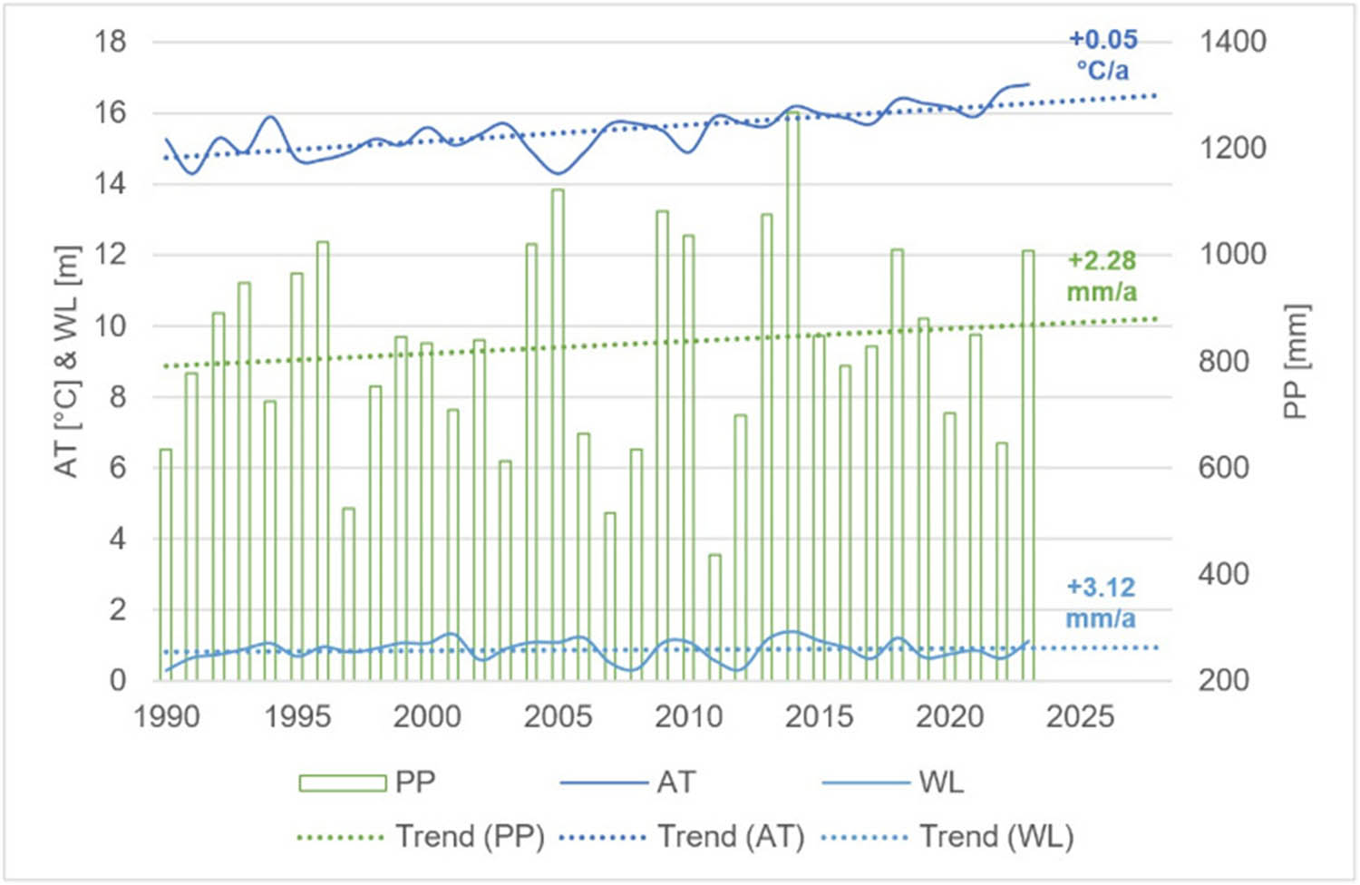
Annual average and trends of AT, PP, and WL during 1990–2023.
During our research period, elevated WL prevented significant interchange between sea and lake water, with the lowest monthly average measured at 0.69 MASL (Figure 2). WL values were higher than historical averages due to heavy rainfall in May 2023 and subsequently dropped below historic averages in January and February 2024, which we attributed to lower monthly PP at the end of 2023 and the beginning of 2024. This downward trend continued into early spring 2024, leading to further decreases in WL during May and June. Throughout the research, average monthly AT remained consistently higher than historic averages (Figure 2).
3.2 Assessing vertical and temporal variability in water column data
We collected vertical profiles at the northern lake station (Figure 1a – point marked as “Vertical profile” at 15°30′40″E, and 43°55′41″N, WGS84) on March 15th and July 19th, 2024. On March 15th, we measured a water depth of 2.95 m with a WL of 1.41 MASL, while on July 19th, the depth decreased to 2.12 m with a WL of 0.58 MASL (Figure S1). We also observed the temporal sensitivity of parameters at the same monitoring site at 30 min intervals (Figure S2). Despite the difference in water depth and time frame of the two measurements, we found that the readings from both dates were comparable in relative units, indicating temporal sensitivity with change per hour and vertical variability with change per meter.
We observed that salinity and EC remained stable across all depths and time throughout our campaigns, with negligible differences of ≤0.01 in their respective units between the lowest and highest values for each parameter. We observed a slight increase in DO over time, with rates of 0.04 mg/L per hour in March and 0.12 mg/L per hour in July, while depth had little effect on it (decrease of 0.02 mg/L per meter in March and decrease of 0.07 mg/L per meter in July). WT and SO decreased with depth, showing a decrease of 0.44°C per meter for WT and 1.11% per meter for SO in March and a decrease of 0.17°C per meter for WT and 1.15% per meter for SO in July. However, both parameters increased over time due to changes in AT, with an increase of 0.31°C per hour for WT and 1.20% per hour for SO in March and increase of 0.21°C per hour for WT and 1.73% per hour for SO in July. We also recorded fluctuations in Chl-a and turbidity, with Chl-a increasing by 0.45 µg/L per meter in March and 0.35 µg/L per meter in July. Turbidity experienced an increase of 0.52 FNU per meter in March and 0.49 FNU per meter in July, with gradual decline over time (decrease of 0.10 FNU per hour in March and 0.03 FNU per hour in July).
3.3 Seasonal and spatial variations in water quality parameters and their correlation with meteorological data
During the research period, all meteorological and WL data, except PP, exhibited normal distribution based on the Jarque–Bera test (Table S2). We transformed the PP variable using a cube root to achieve a normality. All water quality parameters had p-values below the 0.05 significance threshold, indicating non-normal distribution. While various transformations yielded marginal improvements, only the Chl-a parameter gained normal distribution following a square root transformation. Due to the predominance of non-normal distributions, we conducted our analysis of monthly water quality data using median values. We employed the median absolute deviation (MAD) to assess variation, as it is less sensitive to outliers compared to standard deviation [30]. Table S3 presents a comprehensive overview of the data distribution, presenting mean and median values alongside standard deviation and MAD. Our calculations were based on a maximum of 20 monitoring stations in the lake per date, and the quantity of measured data stations per date varied (Table S3).
We observed that Chl-a varied from 0.15 μg/L in April 2023 to 2.39 μg/L in November 2023, with a mean value of 0.94 ± 0.39 μg/L and median value of 0.90 ± 0.24 μg/L (Table S3). The range of Chl-a levels was 2.24 μg/L, with the maximum and minimum values differing almost 2.5 times the median. In June 2024, we measured the lowest EC value of 2.66 dS/m, which peaked in November 2023 at 4.80 dS/m, showing a gradual decrease by the end of our research period (Table S3, Figure 5). The mean and median EC measurements were 3.96 ± 0.65 dS/m and 4.19 ± 0.49 dS/m, respectively, with a range differing by 2.14 dS/m. This range represents 45 and 51% of the highest value and median value, respectively. The mean and median in situ values for salinity were 2.10 ± 0.36 and 2.22 ± 0.28, respectively, with values ranging from 1.37 in June 2024 to 2.58 in November 2023 (Table S3, Figure 5). The salinity values showed a 1.21 variation, accounting for 47 and 55% of the highest and median values, respectively.
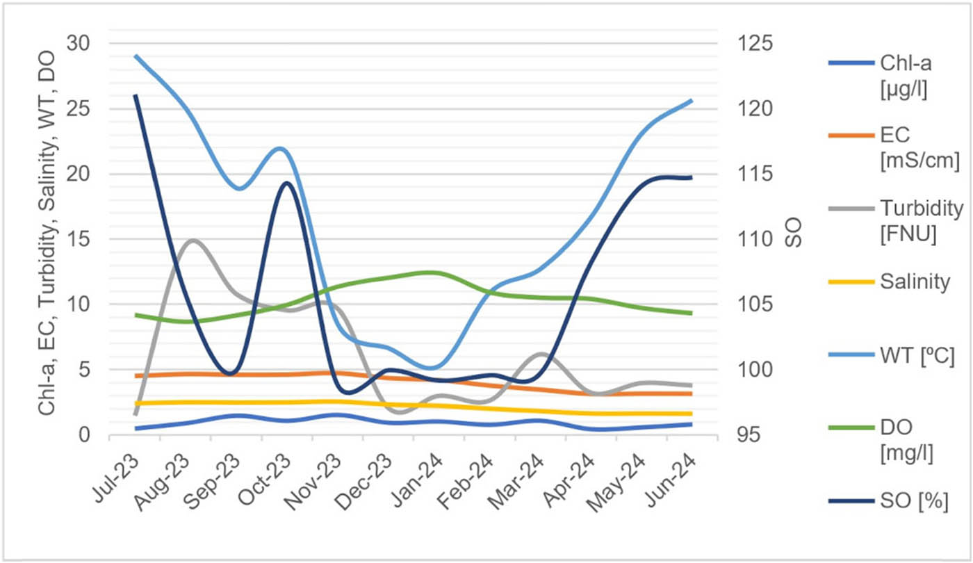
Median values of water quality parameters from the dataset (Chl-a, EC, turbidity, salinity, WT, DO, SO).
We measured the turbidity levels ranging from 0.73 FNU in July 2023 to 15.93 FNU in August 2023, with a mean value of 5.76 ± 3.96 FNU and median value of 3.85 ± 1.63 FNU. Over this 12-month period, we observed a range of turbidity values of 15.20 FNU, which accounts for 95% of the maximum value and 395% of the median value. In July 2023, we measured the highest WT (30.22°C), which declined to 4.47°C in January 2024, with a mean of 16.98 ± 7.87°C and a median of 17.16 ± 7.33°C. The WT data exhibited a fluctuation of 25.75°C, representing 85 and 150% of the maximum and median values, respectively.
We observed that DO levels ranged from 7.60 mg/L in August 2023 to 12.60 mg/L in January 2024, with a mean value of 10.33 ± 1.15 mg/L and a median of 10.35 ± 0.85 mg/L. During this period, DO values fluctuated within a range of 5 mg/L, which represented 40 and 48% of the maximum and median values, respectively. We observed that SO decreased to 93.46% in December 2023 after reaching a high of 143.28% in July 2023. A mean of SO is 106.70 ± 8.85% and a median is 103.64 ± 4.95%, while the SO values ranged from 49.82%, which is equivalent to 35% of the highest value and 48% of the median value.
Spearman’s correlation analysis revealed that the daily vertical movement of phytoplankton (Figure S1), influenced by factors like SH, WS, water column mixing, and PP, leads to changes in Chl-a concentrations (Figure 6a). Notably, we observed higher Chl-a levels in November compared to July (Figure 5), but we found no significant correlation between Chl-a and DO levels (Figure 6b), likely due to unpredictable fluctuations from factors such as the absence of macrophytes and phytoplankton accumulation. Our study revealed that EC, salinity, and turbidity significantly impact the Chl-a values across the lake (Figure 6b). We found that factors such as WT, total dissolved solids, PP, flooding, evaporation, and water flow have an impact on EC and salinity levels. Increased water volume and level can reduce EC and salinity (Figure 6a).
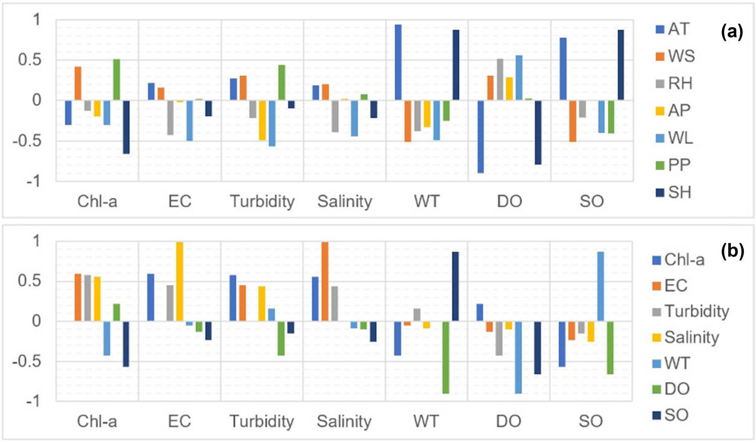
Spearman’s coefficient of determination between: (a) WL, meteorological (AT, WS, RH, AP, PP, SH), and water quality parameters (Chl-a, EC, turbidity, salinity, WT, DO, SO) and (b) in-between water quality parameters (Chl-a, EC, turbidity, salinity, WT, DO, SO).
We found that turbidity can lead to increased WT and decreased DO levels (Figure 6b). We recognized that factors such as PP and WS can further impact turbidity by increasing stream volume and resuspending settled sediments (Figure 6a). Turbidity will often spike annually due to spring rains (Figure 5) and snowmelt. Sunlight and AT primarily influence WT in Vrana Lake (Figure 6a). We measured higher WT during summer, autumn, and spring, and lower temperatures during colder months (Figure 5). Warmer waters have higher EC, but colder waters can hold more DO and have lower levels of SO (Figure 6b).
Aeration sources such as wind, AT (Figure 6a), photosynthetic activity, and oxygen consumption by aquatic organisms influence the levels of DO in waterbodies. DO levels can vary based on WT (Figure 6b), water pressure, and salinity, with fluctuations occurring due to microbial breakdown and limited air contact. DO levels are higher in winter and lower in summer (Figure 5). SO levels are around or slightly exceed 100% throughout the year (Table S3 and Figure 5).
3.3.1 Spatial distribution
According to equation (3), we found that the coarsest grid resolution is approximately 300 m when considering 20 unevenly distributed monitoring stations in an area of approximately 30 km2. The comparison of 15 GIS spatial interpolation methods revealed that the Global Polynomial Interpolation – Second order method achieved the lowest RMSE for Chl-a, while SK – Optimized achieved the lowest RMSE for EC, salinity, DO, and SO (Table S4, Figure S3). EBK – Advanced had the lowest RMSE for turbidity, and SK – Default had the lowest RMSE for WT (Table S4). Generally, Kriging methods outperformed deterministic interpolation methods regarding RMSE values, with EBK – Advanced and all SK methods ranking in the top five for average rank across all parameters. Overall, SK – Optimized ranked as the best for lowest RMSE using equation (1) across all parameters (Table S5). We calculated ME values using equation (2), and both Inverse Distance Weighted methods and EBK – Default consistently scored 0, indicating the highest accuracy (Table S4). However, when we considered the ranking of all GIS spatial interpolation methods, we found that SK – Trend emerged as the most suitable method for modelling all parameters (Table S5). We used this method to create distribution maps demonstrating the variability of water quality parameters (Figure 7).
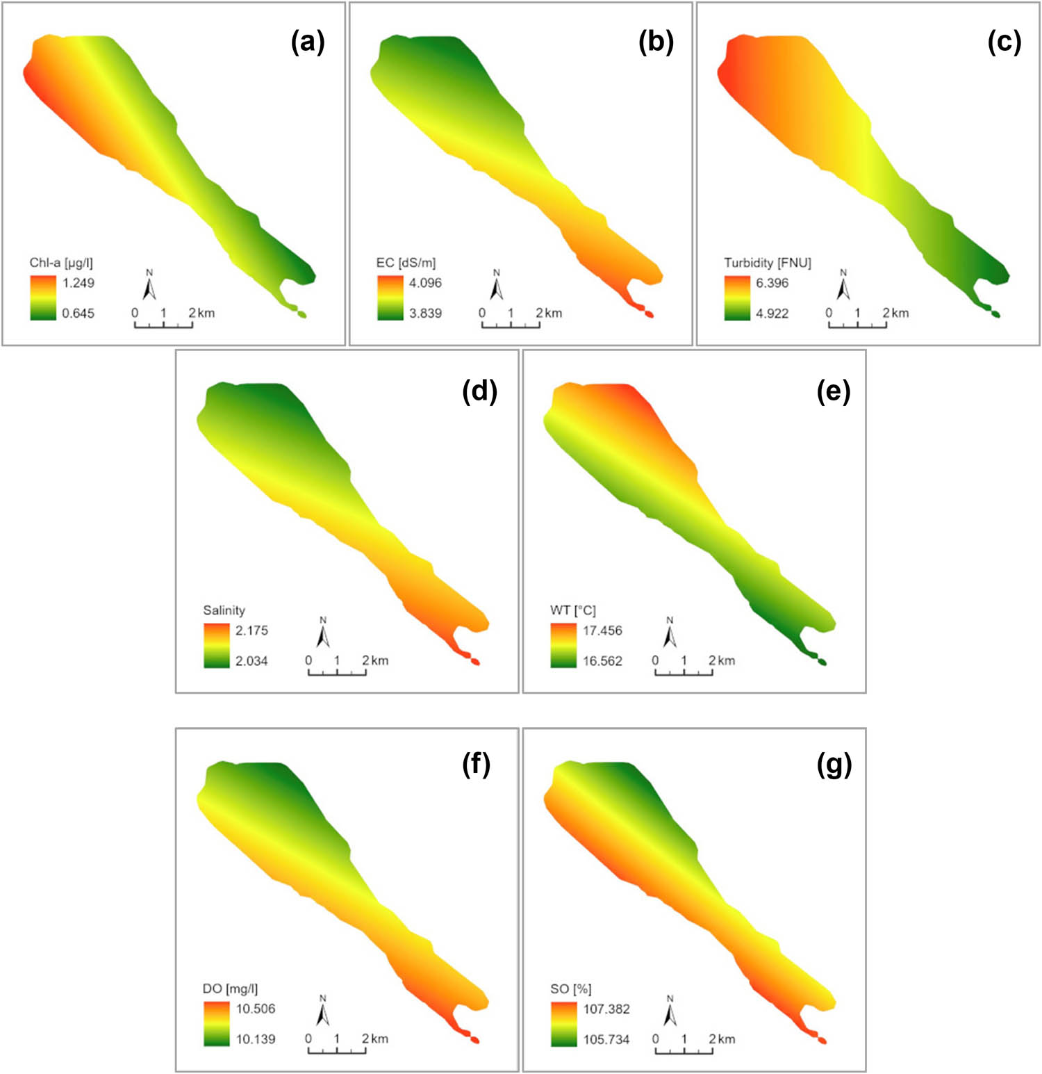
SK – Trend interpolation showing parameter distributions: (a) Chl-a, (b) EC, (c) turbidity, (d) salinity, (e) WT, (f) DO, and (g) SO.
We observed that Chl-a concentrations peak in the northwestern region of the lake, particularly near the Kotarka channel, which serves as the main freshwater tributary (Figure 7a). Conversely, we found that the eastern part of the lake, being the shallowest (Figure 1a), consistently maintained lower Chl-a levels throughout the year (Figure 7a). Turbidity was the highest in the northwestern part of the lake, near the Kotarka channel, while the southeastern part exhibited the lowest turbidity levels (Figure 7c).
There was a strong correlation between EC and salinity in the lake, with both parameters exhibiting similar distribution patterns. The southern region, connected to the sea through the Prosika canal, experienced seawater intrusion, especially during warmer months with lower WL. This resulted in higher EC and salinity in the south and lower EC levels in the north (Figure 7b and d).
We monitored the lake in a counterclockwise direction, starting at station 4 and ending at station 2 (Figure 1a), which took us approximately 3 h. During this process, WT and SO levels gradually increased, influenced by AT (Figure S2). This resulted in higher WT at later monitoring stations and in shallower areas on the northern and eastern sides of the lake (Figure 7e). DO levels were highest in the southern, deepest part of the lake near the Prosika canal and lowest in the northern area near the freshwater tributary Lateral channel (Figure 7f). Similarly, SO levels were highest in the deep western part of the lake and lowest in the shallow northeastern region (Figure 7g).
4 Discussion
4.1 Impact of climate change on Vrana Lake
Historical data indicate rising global temperatures and extreme weather events, including heavy precipitation. Our study confirms the growing trend of overall AT from the early 1990s till 2020s (2.11°C in 34 years) anticipated by IPCC [3], impacting ecosystems and affecting lake water quality. PP levels exhibit significant variability from average values, reflecting the occurrence of extreme weather events throughout the years, such as drought years and flooding years. Rising WL trend may be influenced by the Adriatic Sea’s mean sea level rise of +2.6 mm/year from 1993 to 2019, as reported by Pandžić et al. [50]. Given Vrana Lake’s connection to the sea through the Prosika canal, it is especially vulnerable to sea-level changes – a trend also observed in other coastal lakes, such as those in the Netherlands [51]. Our trend analysis, based on the work of Rubinić and Katalinić [39], which covers the period from 1961 to 2010, indicates a similar increase in AT and lake WL.
4.2 Vertical stratification and water quality dynamics
Vertical profiles revealed a very well-mixed water column with minimal or no stratification. This aligns with findings by Holgerson et al. [52], who reported that shallow lakes over 4 ha in surface tend to experience frequent mixing driven by wind and convection, preventing sustained stratification. In Vrana Lake, we measured slightly elevated Chl-a and turbidity at greater depths with lower light availability, a pattern also observed by Girdner et al. [53]. Similar to the observations in Lake Taihu [54] and Siombak Lake [55], where vertical WT differences were typically within 1°C and showed no significant variation in DO across the water column, we observed that Vrana Lake also exhibits very limited vertical WT gradients and minimal variations in DO, confirming its classification as a shallow, well-mixed system. Likewise, the stability of salinity throughout the water column mirrors observations in shallow saline Lake Shunet in Russia [56], where salinity remains stable to depths of 5 m. Given the shallow nature of Vrana Lake, we find that vertical variations are not significant and can be disregarded, allowing us to use median values from vertical profiles as reference measures for each monitoring station.
4.3 Seasonal and spatial variations in water quality and meteorological influences
The spatial distribution of water quality parameters is important for understanding changes in water quality across a lake. Our findings indicate a slight increase in Chl-a concentrations outside the vegetation period, particularly during autumn and winter. This is consistent with a study by Kong et al. [57], in which it was found that phytoplankton growth in winter is particularly sensitive to light and temperature changes, making it vulnerable to the impacts of climate change.
According to the legislation in The Official Gazette [58], our 12-month study of Vrana Lake shows that it is mesotrophic (classified as “very good” based on eutrophication indicators for mean annual Chl-a values). This differs from the 2021 measurements from Hrvatske vode, which classified the lake as mesotrophic/eutrophic (classified as “good”) [40]. We acknowledge that the reliability of Chl-a measurements in our study is uncertain due to the use of the multiparameter probe without spectrophotometric analysis of water samples. A study by Zolfaghari et al. [45] shows that the connections between sonde and laboratory measurements of Chl-a depend on the site and the methods used in the laboratory.
Salinity concentrations in Vrana Lake rise due to evaporation and the entry of seawater, particularly during the summer (Figure 5), as demonstrated by recent findings in another coastal lake in Croatia [59]. While the Lateral channel remains fresh, heavy rainfall can introduce slightly saline water into the Kotarka channel due to the spring from Vrana polje in the north [35]. Seasonal changes, such as reduced seawater influx during colder periods and potential salinity changes in the Kotarka channel, further affect water quality.
Turbidity levels in Vrana Lake are influenced by factors like nutrient and water flow from tributaries, with warmer months leading to increased turbidity due to lower WLs and active vegetation periods. Contributing sources include soil erosion, seasonal variations, local geology, and algal blooms, which can negatively impact water quality and aquatic life [60]. Additionally, higher turbidity level in the northwestern part of the lake may be linked to the anthropogenic influence, as reported by Silva et al. [61], including nearby road network and industries.
WT is affected by AT and SH, showing higher temperatures in shallow parts of the lake, as found by Anamunda and Lamtane [62]. WT variations have effect on the DO and SO levels, biological activities, and other parameters, as reported by Wang et al. [63] and Khouni et al. [19]. Areas with higher Chl-a concentrations generally have elevated DO levels, which inversely correlate with WT and AT, as found by Saturday et al. [64]. In shallow lakes like Vrana Lake, higher DO levels are typically associated with increased SO concentrations, and SO levels typically remain near 100% or slightly above, sustained by photosynthesis, aeration, and shallow mixing [65], as found by Allesson et al. [66].
5 Conclusion
Our study of Vrana Lake reveals significant impacts of climate change on water quality and ecosystem dynamics. Long-term trends show increasing AT, PP, and WL, suggesting a complex interaction influenced by rising sea levels from the Adriatic Sea. Due to the lake’s shallow nature and minimal vertical stratification, median values from vertical profiles are sufficient for station-level monitoring.
We observed seasonal variability in turbidity, EC, and Chl-a, with a shift from mesotrophic/eutrophic to mesotrophic conditions, emphasizing the need for continuous monitoring. Additionally, we identify the SK – Trend method as the most effective GIS spatial interpolation method for modelling water quality parameters, based on RMSE and ME rankings.
Limitations of our study include exclusive use of the YSI EXO2 multiparameter probe and the absence of water sampling for laboratory analysis. In the absence of macrophytes, Chl-a measurements accuracy could be improved through spectrophotometry and phytoplankton identification. While we found turbidity to be a useful water quality indicator, incorporating a Secchi disk for assessing water clarity would have been advantageous. The expanded monitoring network supports subsequent remote sensing and machine learning analyses; however, selecting a subset of optimal stations based on GIS multicriteria analysis in future studies could improve cost-efficiency.
We recommend that future research on Vrana Lake addresses these limitations, identifies specific phytoplankton and macrophyte species, and prioritizes vertical stratification analysis and water quality dynamics before modelling water quality. Given the strong correlation between EC and salinity, and the fact that salinity is derived from EC measurements using the EXO2 probe, we recommend using EC as the primary parameter in similar studies.
Overall, our findings underscore the complex environmental interactions shaping Vrana Lake’s ecosystem and the necessity for adaptive management in response to climate change. Our findings are particularly relevant to institutions responsible for monitoring Vrana Lake, including the Water Institute Josip Juraj Strossmayer and the Public Institution Vransko Jezero Nature Park. They may also benefit other authorities and researchers engaged in future studies on Lake Vrana and other coastal shallow lakes. Our research lays the groundwork for future studies using GIS multicriteria analysis, remote sensing, and machine learning to improve lake management and address ecological challenges.
Acknowledgments
We would like to thank Vesna Stipaničev, PhD, and the team of researchers from the Water Institute Josip Juraj Strossmayer, Dario Rogić and the team from the Public Institution Vransko Jezero Nature Park, as well as Tomislav Bulat and the team from the Ruđer Bošković Institute, for their valuable support in collecting in situ data. We would also like to thank Hrvatske Vode for providing the bathymetry data, and the Croatian Meteorological and Hydrological Service for providing the meteorological data. Finally, we extend our gratitude to Assoc. Prof. Andrija Krtalić, PhD, and Assoc. Prof. Ante Šiljeg, PhD, for their guidance on the structure of the manuscript. This study was supported by the SMART-Water project HR-BA-ME00330.
-
Funding information: This research was funded by the Interreg VI-A IPA Croatia-Bosnia and Herzegovina-Montenegro program 2021–2027 under Interreg Self-sustainable Multisensor System for Monitoring Water Quality in Inland Waterbodies (SMART-Water) project HR-BA-ME00330. The funding covered the analysis and interpretation of data; writing the research; and the decision to submit the article for publication. The acquired skills, knowledge, and results from this research were used to meet the needs of the SMART-Water project.
-
Author contributions: All authors contributed to the study conception and design. All authors performed data collection, A.B. performed data analyses, and N.C. and M.Ć.D. performed data validation. N.C. performed supervision. A.B. prepared the manuscript with contributions from all co-authors. The authors applied the SDC approach for the sequence of authors.
-
Conflict of interest: Authors state there is no conflict of interest.
-
Supplemental information: Spatiotemporal Water Quality Analysis of Vrana Lake SI.docx.
-
Dataset: Batina A, Cukrov N, Ćuže Denona M. Assessing Water Quality Dynamics in Vrana Lake 2024. https://doi.org/10.17632/82crs2ssss.1.
-
Data availability statement: The authors confirm that the datasets that support the findings of this research are publicly available and all sources are cited in the text and generated data, which are further analysed is available within the article.
References
[1] Hou P, Chang F, Duan L, Zhang Y, Zhang H. Seasonal variation and spatial heterogeneity of water quality parameters in lake Chenghai in Southwestern China. Water. 2022;14:1640. 10.3390/w14101640.Search in Google Scholar
[2] Chen F, Li S, Song K. Remote sensing of lake chlorophyll-a in Qinghai-Tibet Plateau responding to climate factors: Implications for oligotrophic lakes. Ecol Indic. 2024;159:111674. 10.1016/j.ecolind.2024.111674.Search in Google Scholar
[3] IPCC. Climate Change 2023: Synthesis Report. Contribution of working groups I, II and III to the sixth assessment report of the intergovernmental panel on climate change [Core Writing Team, H. Lee and J. Romero (eds.)]. First. Geneva, Switzerland: Intergovernmental panel on climate change; 2023. p. 1–34. 10.59327/IPCC/AR6-9789291691647.001.Search in Google Scholar
[4] Li Z, Zhang Z, Xiong S, Zhang W, Li R. Lake surface temperature predictions under different climate scenarios with machine learning methods: A case study of Qinghai lake and Hulun lake, China. Remote Sens. 2024;16:3220. 10.3390/rs16173220.Search in Google Scholar
[5] Wu Q, Xia X, Li X, Mou X. Impacts of meteorological variations on urban lake water quality: a sensitivity analysis for 12 urban lakes with different trophic states. Aquat Sci. 2014;76:339–51. 10.1007/s00027-014-0339-6.Search in Google Scholar
[6] Rezaee A, Mosaedi A, Beheshti A, Zarrin A. Using wavelet transform to analyze the dynamics of climatic variables; to assess the status of available water resources in Iran (1961–2020). Earth Sci Inf. 2024;17:5499–519. 10.1007/s12145-024-01433-0.Search in Google Scholar
[7] Vasistha P, Ganguly R. Assessment of spatio-temporal variations in lake water body using indexing method. Env Sci Pollut Res. 2020;27:41856–75. 10.1007/s11356-020-10109-3.Search in Google Scholar PubMed
[8] Uslu A, Dugan ST, El Hmaidi A, Muhammetoglu A. Comparative evaluation of spatiotemporal variations of surface water quality using water quality indices and GIS. Earth Sci Inf. 2024;17:4197–212. 10.1007/s12145-024-01389-1.Search in Google Scholar
[9] Gautam R, Shrestha SM. Hydrogeochemical evaluation and characterization of water quality in the Phewa Lake, Pokhara, Nepal. Env Sci Pollut Res. 2024;31:60568–86. 10.1007/s11356-024-35213-6.Search in Google Scholar PubMed
[10] Horvat Z, Horvat M, Pastor K. Assessment of spatial and temporal water quality distribution in shallow lakes: Case study for Lake Ludas. Serb Env Earth Sci. 2022;82:11.10.1007/s12665-022-10683-4Search in Google Scholar
[11] Jácome G, Valarezo C, Yoo C. Assessment of water quality monitoring for the optimal sensor placement in lake Yahuarcocha using pattern recognition techniques and geographical information systems. Env Monit Assess. 2018;190:259. 10.1007/s10661-018-6639-x.Search in Google Scholar PubMed
[12] İlhan N, Demir Yetiş A, Yeşilnacar Mİ, Atasoy ADS. Predictive modelling and seasonal analysis of water quality indicators: Three different basins of Şanlıurfa, Turkey. Env Dev Sustainability. 2022;24:3258–92.10.1007/s10668-021-01566-ySearch in Google Scholar
[13] Ding W, Zhao J, Qin B, Wu T, Zhu S, Li Y, et al. Exploring and quantifying the relationship between instantaneous wind speed and turbidity in a large shallow lake: Case study of Lake Taihu in China. Env Sci Pollut Res. 2021;28:16616–32. 10.1007/s11356-020-11544-y.Search in Google Scholar PubMed
[14] Kang J, Yang F, Wang J, Liu Y, Fang D, Jiang C. Spatial-temporal evolution of habitat quality in tropical monsoon climate region based on “pattern–process–quality” – a case study of Cambodia. Open Geosci. 2025;17:20220748. 10.1515/geo-2022-0748.Search in Google Scholar
[15] Wang R, Pan L, Niu W, Li R, Zhao X, Bian X, et al. Monitoring the spatiotemporal dynamics of surface water body of the Xiaolangdi Reservoir using Landsat-5/7/8 imagery and Google Earth Engine. Open Geosci. 2021;13:1290–302. 10.1515/geo-2020-0305.Search in Google Scholar
[16] Li J, Tian L, Wang Y, Jin S, Li T, Hou X. Optimal sampling strategy of water quality monitoring at high dynamic lakes: A remote sensing and spatial simulated annealing integrated approach. Sci Total Environ. 2021;777:146113. 10.1016/j.scitotenv.2021.146113.Search in Google Scholar
[17] Wilkinson AA, Hondzo M, Guala M. Vertical heterogeneities of cyanobacteria and microcystin concentrations in lakes using a seasonal in situ monitoring station. Glob Ecol Conserv. 2020;21:e00838. 10.1016/j.gecco.2019.e00838.Search in Google Scholar
[18] Bayable G, Cai J, Mekonnen M, Legesse SA, Ishikawa K, Sato S, et al. Spatiotemporal variability of lake surface water temperature and water quality parameters and its interrelationship with water hyacinth biomass in Lake Tana, Ethiopia. Env Sci Pollut Res. 2024;31:45929–53. 10.1007/s11356-024-34212-x.Search in Google Scholar PubMed
[19] Khouni I, Louhichi G, Ghrabi A. Use of GIS based inverse distance weighted interpolation to assess surface water quality: Case of Wadi El Bey, Tunisia. Env Technol Innov. 2021;24:101892. 10.1016/j.eti.2021.101892.Search in Google Scholar
[20] Vasistha P, Ganguly R. Water quality assessment in two lakes of Panchkula, Haryana, using GIS: Case study on seasonal and depth wise variations. Env Sci Pollut Res. 2022;29:43212–36. 10.1007/s11356-022-18635-y.Search in Google Scholar PubMed
[21] Murphy RR, Curriero FC, Ball WP. Comparison of spatial interpolation methods for water quality evaluation in the Chesapeake Bay. J Env Eng. 2010;136:160–71. 10.1061/(ASCE)EE.1943-7870.0000121.Search in Google Scholar
[22] Khan M, Almazah MMA, EIlahi A, Niaz R, Al-Rezami AY, Zaman B. Spatial interpolation of water quality index based on Ordinary kriging and Universal kriging. Geomat Nat Hazards Risk. 2023;14:2190853. 10.1080/19475705.2023.2190853.Search in Google Scholar
[23] Vujović F, Ćulafić G, Valjarević A, Brđanin E, Durlević U. Comparative geomorphometric analysis of drainage basin using Aw3d30 model in ArcGIS and QGIS environment: Case study of the Ibar river drainage basin, Montenegro. Agric For. 2024;70(1):217–30. 10.17707/AgricultForest.70.1.15.Search in Google Scholar
[24] Oseke FI, Anornu GK, Adjei KA, Eduvie MO. Assessment of water quality using GIS techniques and water quality index in reservoirs affected by water diversion. Water-Energy Nexus. 2021;4:25–34. 10.1016/j.wen.2020.12.002.Search in Google Scholar
[25] Aleksova B, Lukić T, Milevski I, Spalević V, Marković SB. Modelling water erosion and mass movements (wet) by using GIS-based multi-hazard susceptibility assessment approaches: A case study—Kratovska Reka Catchment (North Macedonia). Atmosphere. 2023;14:1139. 10.3390/atmos14071139.Search in Google Scholar
[26] Durlević U. Assessment of torrential flood and landslide susceptibility of terrain: Case study - Mlava River Basin (Serbia). Glas Srp Geogr Drus. 2021;101:49–75. 10.2298/GSGD2101049D.Search in Google Scholar
[27] Antonakos A, Lambrakis N. Spatial interpolation for the distribution of groundwater level in an area of complex geology using widely available GIS tools. Env Process. 2021;8:993–1026. 10.1007/s40710-021-00529-9.Search in Google Scholar
[28] Boumpoulis V, Michalopoulou M, Depountis N. Comparison between different spatial interpolation methods for the development of sediment distribution maps in coastal areas. Earth Sci Inf. 2023;16:2069–87. 10.1007/s12145-023-01017-4.Search in Google Scholar
[29] Ouabo RE, Sangodoyin AY, Ogundiran MB. Assessment of ordinary kriging and inverse distance weighting methods for modeling chromium and cadmium soil pollution in E-waste sites in Douala, Cameroon. J Health Pollut. 2020;10:200605. 10.5696/2156-9614-10.26.200605.Search in Google Scholar PubMed PubMed Central
[30] Reimann C, Filzmoser P. Normal and lognormal data distribution in geochemistry: death of a myth. Consequences for the statistical treatment of geochemical and environmental data. Env Geol. 2000;39:1001–14. 10.1007/s002549900081.Search in Google Scholar
[31] Batina A, Krtalić A. Integrating remote sensing methods for monitoring lake water quality: A comprehensive review. Hydrol. 2024;11:92. 10.3390/hydrology11070092.Search in Google Scholar
[32] Vuković N, Alegro A, Koletić N, Rimac A, Šegota V Analysis of macrophytes in Vransko Lake from 2010 to 2019 as part of Change We Care project (in Croatian) 2020.Search in Google Scholar
[33] Trbojević I, Šinžar Sekulić J, Subakov Simić G, Milovanović V, Ćuže Denona M, Fressel N, et al. Monitoring of algae from the Characeae family in 2022. Belgrade, Serbia: University of Belgrade, Faculty of Biology (in Serbian); 2022.Search in Google Scholar
[34] Šiljeg A. Digital terrain model in the analysis of geomorphometrical parameters – the example of Nature Park Lake Vrana. Doctoral thesis. Zadar, Croatia: University of Zadar (in Croatian); 2013.Search in Google Scholar
[35] Public Institution Vransko Jezero Nature Park. Management plan for the Nature Park and Special Ornithological Reserve Vransko Lake and its associated ecological network areas (PU 6163) 2023 – 2032 (in Croatian). Biograd na Moru, Croatia: Public Institution Vransko Jezero Nature Park; 2022.Search in Google Scholar
[36] Kurt O. Model-based prediction of water levels for the Great Lakes: A comparative analysis. Earth Sci Inf. 2024;17:3333–49. 10.1007/s12145-024-01341-3.Search in Google Scholar
[37] Croatian Geological Survey. Vrana Lake - Hydrogeological research. Zagreb, Croatia: Croatian Geological Survey, Department of Hydrogeology and Engineering Geology (in Croatian); 2012.Search in Google Scholar
[38] Batina A, Cukrov N, Ćuže Denona M. Assessing water quality dynamics in Vrana Lake [dataset]. Mendeley Data, V1; 2024. 10.17632/82crs2ssss.1.Search in Google Scholar
[39] Rubinić J, Katalinić A. Water regime of Vrana Lake in Dalmatia (Croatia): changes, risks and problems. Hydrol Sci J. 2014;59:1908–24. 10.1080/02626667.2014.946417.Search in Google Scholar
[40] Musić V, Šikoronja M, Tomas D, Varat M. Report on the state of surface waters in 2021. Zagreb, Croatia: Hrvatske vode (in Croatian); 2023.Search in Google Scholar
[41] Planet Team. Planet application program interface: In space for life on earth. San Francisco, CA. https://api.planet.com. 2022.Search in Google Scholar
[42] Li J, Meng Y, Li Y, Cui Q, Yang X, Tao C, et al. Accurate water extraction using remote sensing imagery based on normalized difference water index and unsupervised deep learning. J Hydrol. 2022;612:128202. 10.1016/j.jhydrol.2022.128202.Search in Google Scholar
[43] American Public Health Association. Standard methods for the examination of water and wastewater. 17th edn. Washington, DC, USA: American Public Health Association; 1989.Search in Google Scholar
[44] Xylem. EXO User Manual 2020.Search in Google Scholar
[45] Zolfaghari K, Wilkes G, Bird S, Ellis D, Pintar KDM, Gottschall N, et al. Chlorophyll-a, dissolved organic carbon, turbidity and other variables of ecological importance in river basins in southern Ontario and British Columbia, Canada. Env Monit Assess. 2020;192:1–16. 10.1007/s10661-019-7800-x.Search in Google Scholar PubMed
[46] “Understanding geostatistical analysis.” Esri n.d. https://pro.arcgis.com/en/pro-app/latest/help/analysis/geostatistical-analyst/understanding-geostatistical-analysis.htm (accessed December 17, 2023).Search in Google Scholar
[47] “Exploratory Interpolation (Geostatistical Analyst).” Esri n.d. https://pro.arcgis.com/en/pro-app/latest/tool-reference/geostatistical-analyst/exploratory-interpolation.htm (accessed December 17, 2023).Search in Google Scholar
[48] “Using cross validation to assess interpolation results.” Esri n.d. https://pro.arcgis.com/en/pro-app/latest/help/analysis/geostatistical-analyst/performing-cross-validation-and-validation.htm (accessed April 24, 2024).Search in Google Scholar
[49] Hengl T. Finding the right pixel size. Comput Geosci. 2006;32:1283–98. 10.1016/j.cageo.2005.11.008.Search in Google Scholar
[50] Pandžić K, Likso T, Biondić R, Biondić B. A review of the contribution of satellite altimetry and tide gauge data to evaluate sea level trends in the Adriatic sea within a mediterranean and global context. GeoHazards. 2024;5:112–41. 10.3390/geohazards5010006.Search in Google Scholar
[51] Van Alphen J, Haasnoot M, Diermanse F. Uncertain accelerated sea-level rise, potential consequences, and adaptive strategies in The Netherlands. Water. 2022;14:1527. 10.3390/w14101527.Search in Google Scholar
[52] Holgerson MA, Richardson DC, Roith J, Bortolotti LE, Finlay K, Hornbach DJ, et al. Classifying mixing regimes in ponds and shallow lakes. Water Resour Res. 2022;58:e2022WR032522. 10.1029/2022WR032522.Search in Google Scholar
[53] Girdner S, Mack J, Buktenica M. Impact of nutrients on photoacclimation of phytoplankton in an oligotrophic lake measured with long-term and high-frequency data: implications for chlorophyll as an estimate of phytoplankton biomass. Hydrobiologia. 2020;847:1817–30. 10.1007/s10750-020-04213-1.Search in Google Scholar
[54] Ye R, Shan K, Gao H, Zhang R, Xiong W, Wang Y, et al. Spatio-temporal distribution patterns in environmental factors, chlorophyll-a and microcystins in a large shallow lake, Lake Taihu, China. Int J Env Res Public Health. 2014;11:5155–69. 10.3390/ijerph110505155.Search in Google Scholar PubMed PubMed Central
[55] Leidonald R, Muhtadi A, Lesmana I, Harahap ZA, Rahmadya A. Profiles of temperature, salinity, dissolved oxygen, and pH in Tidal Lakes. IOP Conf Ser: Earth Env Sci. 2019;260:012075. 10.1088/1755-1315/260/1/012075.Search in Google Scholar
[56] Degermendzhy AG, Zadereev ES, Rogozin DY, Prokopkin IG, Barkhatov YV, Tolomeev AP, et al. Vertical stratification of physical, chemical and biological components in two saline lakes Shira and Shunet (South Siberia, Russia). Aquat Ecol. 2010;44:619–32. 10.1007/s10452-010-9336-6.Search in Google Scholar
[57] Kong X, Seewald M, Dadi T, Friese K, Mi C, Boehrer B, et al. Unravelling winter diatom blooms in temperate lakes using high frequency data and ecological modeling. Water Res. 2021;190:116681. 10.1016/j.watres.2020.116681.Search in Google Scholar PubMed
[58] The Official Gazette. Regulation on amendments and supplements to the Regulation on water quality standards. Official Gazette of the Republic of Croatia “Narodne Novine”. 2023;20:1–51 (in Croatian).Search in Google Scholar
[59] Dominović I, Dutour-Sikirić M, Marguš M, Bakran-Petricioli T, Petricioli D, Geček S, et al. Deoxygenation and stratification dynamics in a coastal marine lake. Estuar Coast Shelf Sci. 2023;291:108420. 10.1016/j.ecss.2023.108420.Search in Google Scholar
[60] Fondriest Environmental, Inc. Turbidity, total suspended solids and water clarity. Fundamentals of Environmental Measurements 2014. https://www.fondriest.com/environmental-measurements/parameters/water-quality/turbidity-total-suspended-solids-water-clarity/ (accessed March 14, 2024).Search in Google Scholar
[61] Silva FLD, Stefani MS, Smith W, Schiavone DC, Cunha-Santino MBD, Bianchini I, Jr. An applied ecological approach for the assessment of anthropogenic disturbances in urban wetlands and the contributor river. Ecol Complex. 2020;43:100852. 10.1016/j.ecocom.2020.100852.Search in Google Scholar
[62] Anamunda A, Lamtane HA. Relationship between physicochemical parameters and the abundance of zooplankton in Lake Mweru-Wantipa, Zambia. Int J Bonorowo Wetl. 2022;12(1):33–40. 10.13057/bonorowo/w120104.Search in Google Scholar
[63] Wang Y, Tao J, Zhao L, Qin S, Xiao H, Wang Y, et al. Investigating long-term changes in surface water temperature of Dongting Lake using Landsat imagery, China. Env Sci Pollut Res. 2024;31:41167–81. 10.1007/s11356-024-33878-7.Search in Google Scholar PubMed
[64] Saturday A, Lyimo TJ, Machiwa J, Pamba S. Spatial and temporal variations of phytoplankton composition and biomass in Lake Bunyonyi, South-Western Uganda. Env Monit Assess. 2022;194:288. 10.1007/s10661-022-09954-1.Search in Google Scholar PubMed
[65] Fondriest Environmental, Inc. Dissolved Oxygen. Fondriest 2013. https://www.fondriest.com/environmental-measurements/parameters/water-quality/dissolved-oxygen/ (accessed February 24, 2024).Search in Google Scholar
[66] Allesson L, Valiente N, Dörsch P, Andersen T, Eiler A, Hessen DO. Drivers and variability of CO2:O2 saturation along a gradient from boreal to Arctic lakes. Sci Rep. 2022;12:18989. 10.1038/s41598-022-23705-9.Search in Google Scholar PubMed PubMed Central
© 2025 the author(s), published by De Gruyter
This work is licensed under the Creative Commons Attribution 4.0 International License.
Articles in the same Issue
- Ionization hotspots near waterfalls in Eastern Serbia’s Stara Planina Mountain
- Research Articles
- Seismic response and damage model analysis of rocky slopes with weak interlayers
- Multi-scenario simulation and eco-environmental effect analysis of “Production–Living–Ecological space” based on PLUS model: A case study of Anyang City
- Remote sensing estimation of chlorophyll content in rape leaves in Weibei dryland region of China
- GIS-based frequency ratio and Shannon entropy modeling for landslide susceptibility mapping: A case study in Kundah Taluk, Nilgiris District, India
- Natural gas origin and accumulation of the Changxing–Feixianguan Formation in the Puguang area, China
- Spatial variations of shear-wave velocity anomaly derived from Love wave ambient noise seismic tomography along Lembang Fault (West Java, Indonesia)
- Evaluation of cumulative rainfall and rainfall event–duration threshold based on triggering and non-triggering rainfalls: Northern Thailand case
- Pixel and region-oriented classification of Sentinel-2 imagery to assess LULC dynamics and their climate impact in Nowshera, Pakistan
- The use of radar-optical remote sensing data and geographic information system–analytical hierarchy process–multicriteria decision analysis techniques for revealing groundwater recharge prospective zones in arid-semi arid lands
- Effect of pore throats on the reservoir quality of tight sandstone: A case study of the Yanchang Formation in the Zhidan area, Ordos Basin
- Hydroelectric simulation of the phreatic water response of mining cracked soil based on microbial solidification
- Spatial-temporal evolution of habitat quality in tropical monsoon climate region based on “pattern–process–quality” – a case study of Cambodia
- Early Permian to Middle Triassic Formation petroleum potentials of Sydney Basin, Australia: A geochemical analysis
- Micro-mechanism analysis of Zhongchuan loess liquefaction disaster induced by Jishishan M6.2 earthquake in 2023
- Prediction method of S-wave velocities in tight sandstone reservoirs – a case study of CO2 geological storage area in Ordos Basin
- Ecological restoration in valley area of semiarid region damaged by shallow buried coal seam mining
- Hydrocarbon-generating characteristics of Xujiahe coal-bearing source rocks in the continuous sedimentary environment of the Southwest Sichuan
- Hazard analysis of future surface displacements on active faults based on the recurrence interval of strong earthquakes
- Structural characterization of the Zalm district, West Saudi Arabia, using aeromagnetic data: An approach for gold mineral exploration
- Research on the variation in the Shields curve of silt initiation
- Reuse of agricultural drainage water and wastewater for crop irrigation in southeastern Algeria
- Assessing the effectiveness of utilizing low-cost inertial measurement unit sensors for producing as-built plans
- Analysis of the formation process of a natural fertilizer in the loess area
- Machine learning methods for landslide mapping studies: A comparative study of SVM and RF algorithms in the Oued Aoulai watershed (Morocco)
- Chemical dissolution and the source of salt efflorescence in weathering of sandstone cultural relics
- Molecular simulation of methane adsorption capacity in transitional shale – a case study of Longtan Formation shale in Southern Sichuan Basin, SW China
- Evolution characteristics of extreme maximum temperature events in Central China and adaptation strategies under different future warming scenarios
- Estimating Bowen ratio in local environment based on satellite imagery
- 3D fusion modeling of multi-scale geological structures based on subdivision-NURBS surfaces and stratigraphic sequence formalization
- Comparative analysis of machine learning algorithms in Google Earth Engine for urban land use dynamics in rapidly urbanizing South Asian cities
- Study on the mechanism of plant root influence on soil properties in expansive soil areas
- Simulation of seismic hazard parameters and earthquakes source mechanisms along the Red Sea rift, western Saudi Arabia
- Tectonics vs sedimentation in foredeep basins: A tale from the Oligo-Miocene Monte Falterona Formation (Northern Apennines, Italy)
- Investigation of landslide areas in Tokat-Almus road between Bakımlı-Almus by the PS-InSAR method (Türkiye)
- Predicting coastal variations in non-storm conditions with machine learning
- Cross-dimensional adaptivity research on a 3D earth observation data cube model
- Geochronology and geochemistry of late Paleozoic volcanic rocks in eastern Inner Mongolia and their geological significance
- Spatial and temporal evolution of land use and habitat quality in arid regions – a case of Northwest China
- Ground-penetrating radar imaging of subsurface karst features controlling water leakage across Wadi Namar dam, south Riyadh, Saudi Arabia
- Rayleigh wave dispersion inversion via modified sine cosine algorithm: Application to Hangzhou, China passive surface wave data
- Fractal insights into permeability control by pore structure in tight sandstone reservoirs, Heshui area, Ordos Basin
- Debris flow hazard characteristic and mitigation in Yusitong Gully, Hengduan Mountainous Region
- Research on community characteristics of vegetation restoration in hilly power engineering based on multi temporal remote sensing technology
- Identification of radial drainage networks based on topographic and geometric features
- Trace elements and melt inclusion in zircon within the Qunji porphyry Cu deposit: Application to the metallogenic potential of the reduced magma-hydrothermal system
- Pore, fracture characteristics and diagenetic evolution of medium-maturity marine shales from the Silurian Longmaxi Formation, NE Sichuan Basin, China
- Study of the earthquakes source parameters, site response, and path attenuation using P and S-waves spectral inversion, Aswan region, south Egypt
- Source of contamination and assessment of potential health risks of potentially toxic metal(loid)s in agricultural soil from Al Lith, Saudi Arabia
- Regional spatiotemporal evolution and influencing factors of rural construction areas in the Nanxi River Basin via GIS
- An efficient network for object detection in scale-imbalanced remote sensing images
- Effect of microscopic pore–throat structure heterogeneity on waterflooding seepage characteristics of tight sandstone reservoirs
- Environmental health risk assessment of Zn, Cd, Pb, Fe, and Co in coastal sediments of the southeastern Gulf of Aqaba
- A modified Hoek–Brown model considering softening effects and its applications
- Evaluation of engineering properties of soil for sustainable urban development
- The spatio-temporal characteristics and influencing factors of sustainable development in China’s provincial areas
- Application of a mixed additive and multiplicative random error model to generate DTM products from LiDAR data
- Gold vein mineralogy and oxygen isotopes of Wadi Abu Khusheiba, Jordan
- Prediction of surface deformation time series in closed mines based on LSTM and optimization algorithms
- 2D–3D Geological features collaborative identification of surrounding rock structural planes in hydraulic adit based on OC-AINet
- Spatiotemporal patterns and drivers of Chl-a in Chinese lakes between 1986 and 2023
- Land use classification through fusion of remote sensing images and multi-source data
- Nexus between renewable energy, technological innovation, and carbon dioxide emissions in Saudi Arabia
- Analysis of the spillover effects of green organic transformation on sustainable development in ethnic regions’ agriculture and animal husbandry
- Factors impacting spatial distribution of black and odorous water bodies in Hebei
- Large-scale shaking table tests on the liquefaction and deformation responses of an ultra-deep overburden
- Impacts of climate change and sea-level rise on the coastal geological environment of Quang Nam province, Vietnam
- Reservoir characterization and exploration potential of shale reservoir near denudation area: A case study of Ordovician–Silurian marine shale, China
- Seismic prediction of Permian volcanic rock reservoirs in Southwest Sichuan Basin
- Application of CBERS-04 IRS data to land surface temperature inversion: A case study based on Minqin arid area
- Geological characteristics and prospecting direction of Sanjiaoding gold mine in Saishiteng area
- Research on the deformation prediction model of surrounding rock based on SSA-VMD-GRU
- Geochronology, geochemical characteristics, and tectonic significance of the granites, Menghewula, Southern Great Xing’an range
- Hazard classification of active faults in Yunnan base on probabilistic seismic hazard assessment
- Characteristics analysis of hydrate reservoirs with different geological structures developed by vertical well depressurization
- Estimating the travel distance of channelized rock avalanches using genetic programming method
- Landscape preferences of hikers in Three Parallel Rivers Region and its adjacent regions by content analysis of user-generated photography
- New age constraints of the LGM onset in the Bohemian Forest – Central Europe
- Characteristics of geological evolution based on the multifractal singularity theory: A case study of Heyu granite and Mesozoic tectonics
- Soil water content and longitudinal microbiota distribution in disturbed areas of tower foundations of power transmission and transformation projects
- Oil accumulation process of the Kongdian reservoir in the deep subsag zone of the Cangdong Sag, Bohai Bay Basin, China
- Investigation of velocity profile in rock–ice avalanche by particle image velocimetry measurement
- Optimizing 3D seismic survey geometries using ray tracing and illumination modeling: A case study from Penobscot field
- Sedimentology of the Phra That and Pha Daeng Formations: A preliminary evaluation of geological CO2 storage potential in the Lampang Basin, Thailand
- Improved classification algorithm for hyperspectral remote sensing images based on the hybrid spectral network model
- Map analysis of soil erodibility rates and gully erosion sites in Anambra State, South Eastern Nigeria
- Identification and driving mechanism of land use conflict in China’s South-North transition zone: A case study of Huaihe River Basin
- Evaluation of the impact of land-use change on earthquake risk distribution in different periods: An empirical analysis from Sichuan Province
- A test site case study on the long-term behavior of geotextile tubes
- An experimental investigation into carbon dioxide flooding and rock dissolution in low-permeability reservoirs of the South China Sea
- Detection and semi-quantitative analysis of naphthenic acids in coal and gangue from mining areas in China
- Comparative effects of olivine and sand on KOH-treated clayey soil
- YOLO-MC: An algorithm for early forest fire recognition based on drone image
- Earthquake building damage classification based on full suite of Sentinel-1 features
- Potential landslide detection and influencing factors analysis in the upper Yellow River based on SBAS-InSAR technology
- Assessing green area changes in Najran City, Saudi Arabia (2013–2022) using hybrid deep learning techniques
- An advanced approach integrating methods to estimate hydraulic conductivity of different soil types supported by a machine learning model
- Hybrid methods for land use and land cover classification using remote sensing and combined spectral feature extraction: A case study of Najran City, KSA
- Streamlining digital elevation model construction from historical aerial photographs: The impact of reference elevation data on spatial accuracy
- Analysis of urban expansion patterns in the Yangtze River Delta based on the fusion impervious surfaces dataset
- A metaverse-based visual analysis approach for 3D reservoir models
- Late Quaternary record of 100 ka depositional cycles on the Larache shelf (NW Morocco)
- Integrated well-seismic analysis of sedimentary facies distribution: A case study from the Mesoproterozoic, Ordos Basin, China
- Study on the spatial equilibrium of cultural and tourism resources in Macao, China
- Urban road surface condition detecting and integrating based on the mobile sensing framework with multi-modal sensors
- Review Articles
- Humic substances influence on the distribution of dissolved iron in seawater: A review of electrochemical methods and other techniques
- Applications of physics-informed neural networks in geosciences: From basic seismology to comprehensive environmental studies
- Ore-controlling structures of granite-related uranium deposits in South China: A review
- Shallow geological structure features in Balikpapan Bay East Kalimantan Province – Indonesia
- A review on the tectonic affinity of microcontinents and evolution of the Proto-Tethys Ocean in Northeastern Tibet
- Special Issue: Natural Resources and Environmental Risks: Towards a Sustainable Future - Part II
- Depopulation in the Visok micro-region: Toward demographic and economic revitalization
- Special Issue: Geospatial and Environmental Dynamics - Part II
- Advancing urban sustainability: Applying GIS technologies to assess SDG indicators – a case study of Podgorica (Montenegro)
- Spatiotemporal and trend analysis of common cancers in men in Central Serbia (1999–2021)
- Minerals for the green agenda, implications, stalemates, and alternatives
- Spatiotemporal water quality analysis of Vrana Lake, Croatia
- Functional transformation of settlements in coal exploitation zones: A case study of the municipality of Stanari in Republic of Srpska (Bosnia and Herzegovina)
- Hypertension in AP Vojvodina (Northern Serbia): A spatio-temporal analysis of patients at the Institute for Cardiovascular Diseases of Vojvodina
- Regional patterns in cause-specific mortality in Montenegro, 1991–2019
- Spatio-temporal analysis of flood events using GIS and remote sensing-based approach in the Ukrina River Basin, Bosnia and Herzegovina
- Flash flood susceptibility mapping using LiDAR-Derived DEM and machine learning algorithms: Ljuboviđa case study, Serbia
- Geocultural heritage as a basis for geotourism development: Banjska Monastery, Zvečan (Serbia)
- Assessment of groundwater potential zones using GIS and AHP techniques – A case study of the zone of influence of Kolubara Mining Basin
- Impact of the agri-geographical transformation of rural settlements on the geospatial dynamics of soil erosion intensity in municipalities of Central Serbia
- Where faith meets geomorphology: The cultural and religious significance of geodiversity explored through geospatial technologies
- Applications of local climate zone classification in European cities: A review of in situ and mobile monitoring methods in urban climate studies
- Complex multivariate water quality impact assessment on Krivaja River