Analysis of the equilibrium points and orbits stability for the asteroid 93 Minerva
-
Hu Liu
 ,
Anqi Lang
,
Anqi Lang

Abstract
In this article, we study the orbital dynamics with the gravitational potential of the asteroid 93 Minerva using an irregular shape model from observations. We calculate its physical size, physical mass, surface height, and zero-velocity surface. Meanwhile, we recognize that there are five equilibrium points around Minerva, four of which are external, and one is internal. Two of the external equilibrium points are stable and near the
1 Introduction
Asteroids have extremely high scientific exploration value. Through research and exploration of asteroids, we can further utilize space resources and verify asteroid defense technologies. Since the Galileo spacecraft flew by the 951 Gaspra mission in 1991 (Belton et al. 1992), the exploration of asteroids and comets has come into the spotlight. A number of countries or organizations in the world have completed asteroid visited missions. In 1997, the NEARS (Near Earth Asteroid Rendezvous Shoemaker) probe launched by NASA (National Aeronautics and Space Administration) completed the visit of asteroids such as the asteroid 253 Mathilde (Veverka et al. 1997, 2000). In 2003, JAXA (Japan Aerospace Exploration Agency) launched The Hayabusa probe that visited the asteroid 25143 Itokawa and returned, and this is the first time for humans to obtain a sample of an asteroid (Fujiwara et al. 2006, Abe et al. 2006). In 2004, the Rosetta spacecraft of ESA (European Space Agency) imaged the comet 67P/Churyumov-Gerasimenko and leap past the asteroid 21 Luteria with a distance of 3,160 km (Barucci et al. 2007). In 2012, the Chang’e 2 satellite of CNSA (China National Space Administration) conducted a flyby of 4179 Toutatis asteroid at a distance of 3.2 km (Huang et al. 2013, Zhao et al. 2013, Ji et al. 2015, Zou et al. 2014) and obtained high-definition images of its surface, as shown in Figure 1. In the future, more asteroid exploration missions will be gradually carried out, and become an indispensable step in deep space exploration.
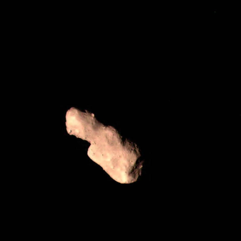
Image of Toutatis by Chang’e 2 engineering camera designed to monitor the state of the solar panel on December 13th, 2012.
Considering the need for asteroid exploration in the solar system, it is of great significance to study the orbital environment around asteroids. Werner and Scheeres (1996) proposed a polyhedral model method to calculate the gravitational force of irregularly shaped asteroids, which was later widely used in the model building of the gravitational field environment of asteroids. Scheeres et al. (1996) applied the Jacobian integral of particles orbiting around asteroids. With the Jacobian integral, we can determine the range of particle motion on the zero-velocity surface. From a practical point of view, it is an important way to understand the orbital dynamics near asteroid by studying the equilibrium points and periodic orbits around an asteroid, and it is also the key to deep space exploration orbits designing. Jiang et al. (2014) proposed a theory of local dynamics around the equilibrium points and classified nondegenerate equilibrium points into different cases. Wang et al. (2014) used the classification proposed by Jiang et al. (2014) to calculate the stability and the topological classification of equilibrium points around 23 asteroids. Yu and Baoyin (2012a) divided the periodic orbits near the equilibrium point in the gravitational field into several topological cases, and then gave a complete classification of periodic orbits. Previous studies have used polyhedral models to analyze the dynamic environment around asteroids, such as 21 Lutetia, 41 Daphne, and 624 Hektor (Mota et al. 2019, Jiang 2018, 2019, Jiang et al. 2018, Moura et al. 2020, Aljbaae et al. 2019). Our goal is to analyze the dynamic environment around binary or triple asteroid systems with large mass ratios, considering the gravitational potential generated by their irregular shapes.
Asteroid 93 Minerva is the fifth triple asteroid system to be discovered, located in the main belt (
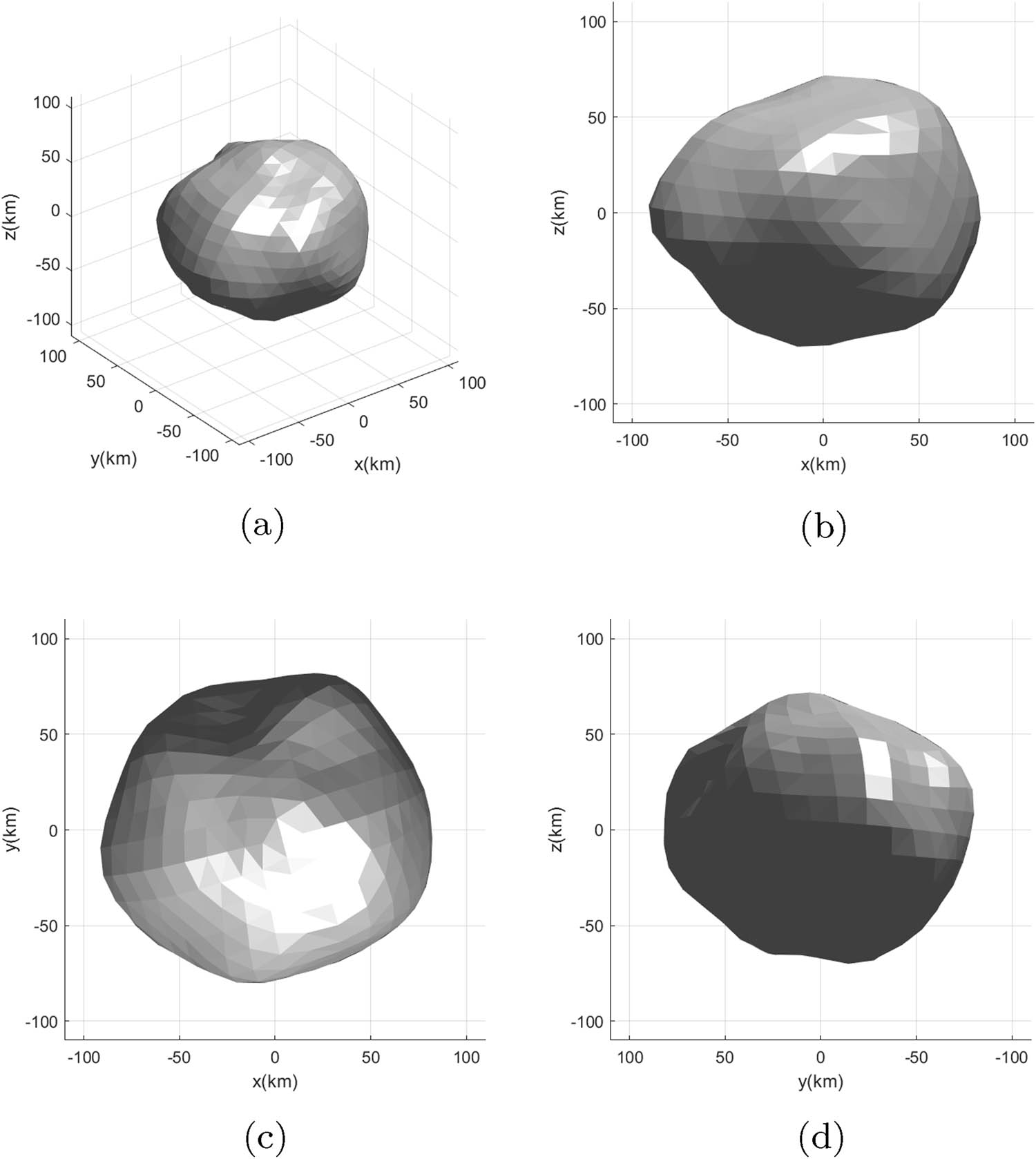
The polyhedron model of asteroid Minerva consists 402 vertices and 800 triangular faces in total. (a) 3D view. (b)
In Section 2, we discuss the physical properties of 93 Minerva, including its physical shape, physical size, and surface height. In addition, we calculate the equilibrium points, zero-velocity surfaces, equilibrium points eigenvalues, and their corresponding topological cases. In Section 3, we analyze the changes in the equilibrium points when the spin speed and the density of the asteroid change. When the spin speed is gradually increased to 2.42 times, it is found that the number of equilibrium points will first increase and then decrease. When the density changes, the topological cases of the equilibrium points also changes, which means the stability changes. Section 4 presents the simulation of the moonlet orbits under the Minerva gravitational potential. The gravitational potential of Minerva was calculated by using the polyhedron model and observational data. Section 5 briefly reviews the findings of the study.
2 Equations of motion and equilibrium points
In this section, we first built the three-dimensional model of Minerva and calculated the physical size, physical mass, and surface height. Then, we discussed the equations of motion, the equilibrium points, and eigenvalues of the equilibrium points around a uniformly rotating object, and calculated the equilibrium points and their eigenvalues of Minerva. Then we analyzed the stability of the equilibrium points.
2.1 Physical model
Since the gravity ratio of the two moonlets to the main asteroid is too small and the distance from the main asteroid is too far, we ignored moonlets gravity when calculating the equilibrium points. We used the polyhedral model method for calculations (Werner and Scheeres 1996), and this model of the asteroid Minerva contains 402 vertices and 800 triangular faces (Marchis et al. 2013).
We translate and rotate the model of the asteroid. The centroid of the asteroid coincides with the origin of the coordinate system. The axes
The bulk density of Minerva is estimated to be
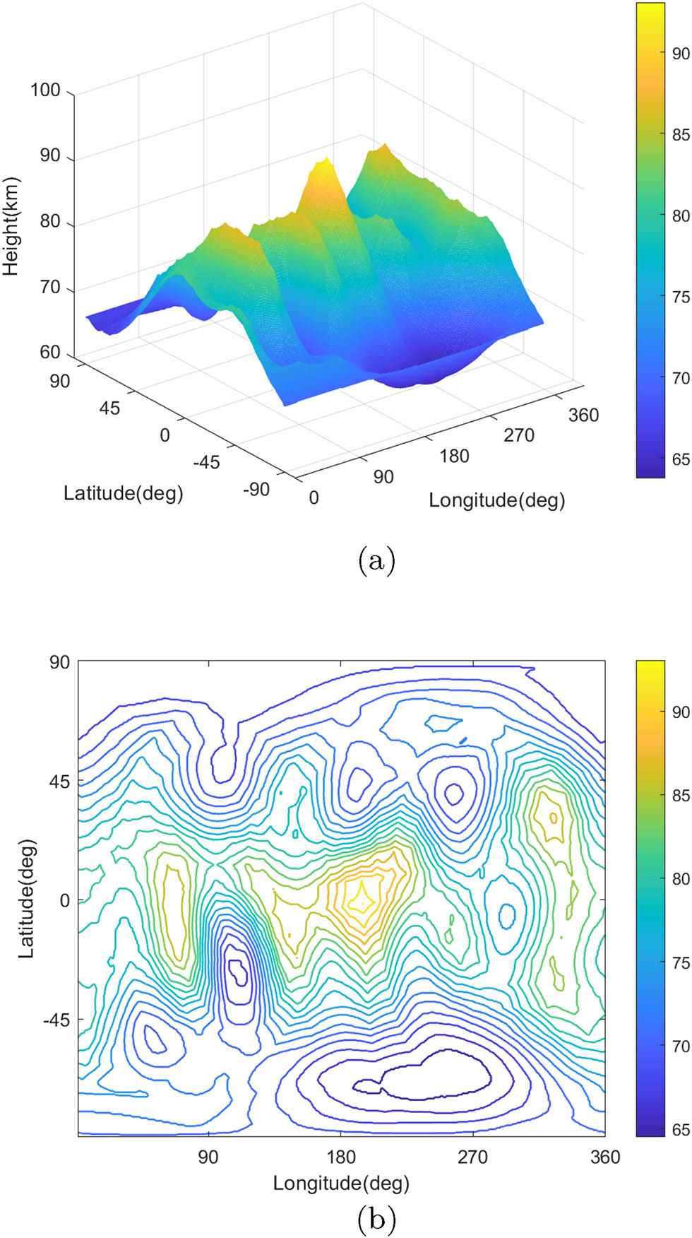
Surface height of Minerva, and the units on the colorbar are km. (a) 3D plot and (b) contour plot.
Surface height refers to the distance between the centroid of the asteroid and a point on the surface with a fixed latitude and longitude. By performing calculations on the polyhedral model, we obtained the surface height data for Minerva, as shown in Figure 3. From the surface height data, we can see that the value range of the surface height is 63.7–93.1 km, and the average value is about 74.4 km. At the same time, the ratio of the maximum to the minimum surface height is about 1.5, which is much smaller than most asteroids. In addition, we can see from the contour map significantly that there are four convex areas and six concave areas on the surface of the asteroid, and these irregular areas made a contribution to the uneven gravity of Minerva.

Locations of the equilibrium points of asteroid Minerva. (a) The positions of the equilibrium points in space. (b) Zero-velocity curves and projections of the equilibrium points in the
2.2 Calculation of equilibrium points
We calculated the equilibrium points and zero-velocity surface in the asteroid’s gravitational potential. When massless particles move in an asteroid’s gravitational potential, we can describe its equation of motion in Cartesian coordinates. The spin speed of the asteroid is
The gravitational potential
Among them,
We can see from this equation, if
Substituting it into Eq. (1), we can obtain
For asteroids with uniform spin, the aforementioned formula can be simplified to
At the same time, the Jacobi function can be expressed by the effective potential as follows:
The zero-velocity surface is an important concept when studying the particle motion interval, and it can be defined by the following equation (Scheeres et al. 1996, Yu and Baoyin 2012b):
The equilibrium points are the critical points of the effective potential
The equilibrium points information of Minerva is shown in Table 1. From Table 1, we found that the equilibrium points are not on the equatorial plane, because Minerva is not north-south symmetry. The positions of the equilibrium points in space are shown in Figure 4(a), and they are approximately evenly distributed around Minerva. The zero-velocity surfaces and projections of equilibrium points in the
Positions of the equilibrium points around Minerva
| Equilibrium points |
|
|
|
|---|---|---|---|
| E1 | 133.582 |
|
|
| E2 |
|
135.744 |
|
| E3 |
|
|
0.398907 |
| E4 | 3.48440 |
|
0.266672 |
| E5 | 0.533699 |
|
|
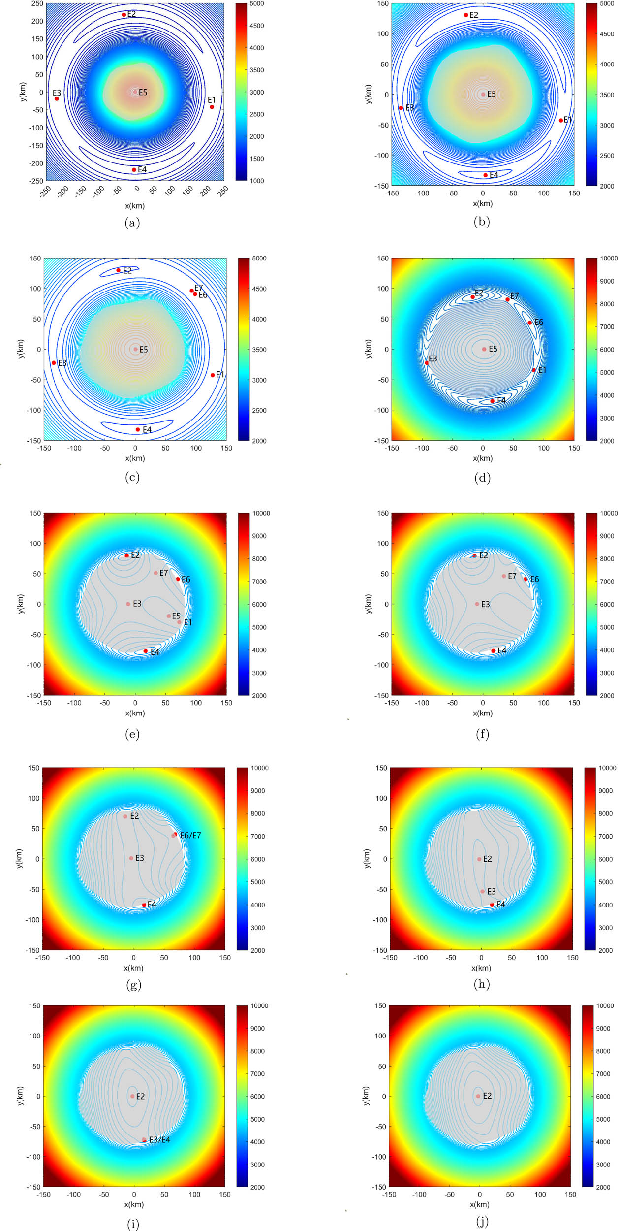
Some typical locations of equilibrium points of asteroid Minerva when increasing the spin speed. (a)
2.3 Eigenvalues of equilibrium points
Denote point
The detailed calculation process is in Appendix A. The calculated eigenvalues of the asteroid Minerva are presented in Table 2.
Eigenvalues of the equilibrium points around Minerva
| Equilibrium points |
|
|
|
|
|
|
|---|---|---|---|---|---|---|
| E1 |
|
|
|
|
0.096861 |
|
| E2 |
|
|
|
|
|
|
| E3 |
|
|
|
|
0.117155 |
|
| E4 |
|
|
|
|
|
|
| E5 |
|
|
|
|
|
|
The topological cases of the equilibrium points can be determined by the following distributions of eigenvalues shown in Table 3 (Jiang et al. 2014, Wang et al. 2014), case 1 is stable, and other cases are unstable. From Table 3, we can see that E1 and E3 belong to case 2, and E2, E4, and E5 belong to case 1. Therefore, among the five equilibrium points of Minerva, E2, E4, and E5 are linearly stable equilibrium points, and E1 and E3 are unstable equilibrium points.
Topological classification of equilibrium points in the gravitational potentials of asteroids
| Topological cases | Eigenvalues | Stability |
|---|---|---|
| Case 1 |
|
Linearly stable |
| Case 2 |
|
|
| Case 3 |
|
|
| Case 4a |
|
|
| Case 4b |
|
|
| Case 5 |
|
|
3 Changes of equilibrium points during the variety of parameters
When we change the parameters of the asteroid, its gravitational field and dynamics environment also change. For equilibrium points, bifurcations and annihilation may occur (Jiang and Baoyin 2018). We analyze the influences on the equilibrium points of Minerva by changing the spin speed and density.
3.1 The change of spin speed
We observed the movement of the equilibrium point positions when the spin speed
The projection of the equilibrium points of asteroid Minerva in the
As Figure 5 shows, when the spin speed changes, the number and positions of the equilibrium points also change gradually. When
As the spin speed continues to vary, E6 and E7 move toward each other, and the second annihilation occurs; meanwhile, E2 comes into the body. When
Jiang and Baoyin (2018) discussed the annihilation of relative equilibrium points in the gravitational field of irregular-shaped asteroids. Ten asteroids were been simulated, and the results are presented in Table 4. When the spin speed increases, the number of equilibrium points will only decrease in most asteroids, but 2063 Bacchus and 1682 Q1 Halley will increase first and then decrease, which is similar to Minerva.
The trend of the equilibrium points number of ten asteroids when the spin speed increases
| Serial number | Asteroids | Diameters (km) | Number trend |
|---|---|---|---|
| 1 |
|
|
|
| 2 |
|
|
|
| 3 |
|
|
|
| 4 |
|
|
|
| 5 |
|
|
|
| 6 |
|
|
|
| 7 |
|
|
|
| 8 |
|
|
|
| 9 |
|
|
|
| 10 | 1P/Halley |
|
|
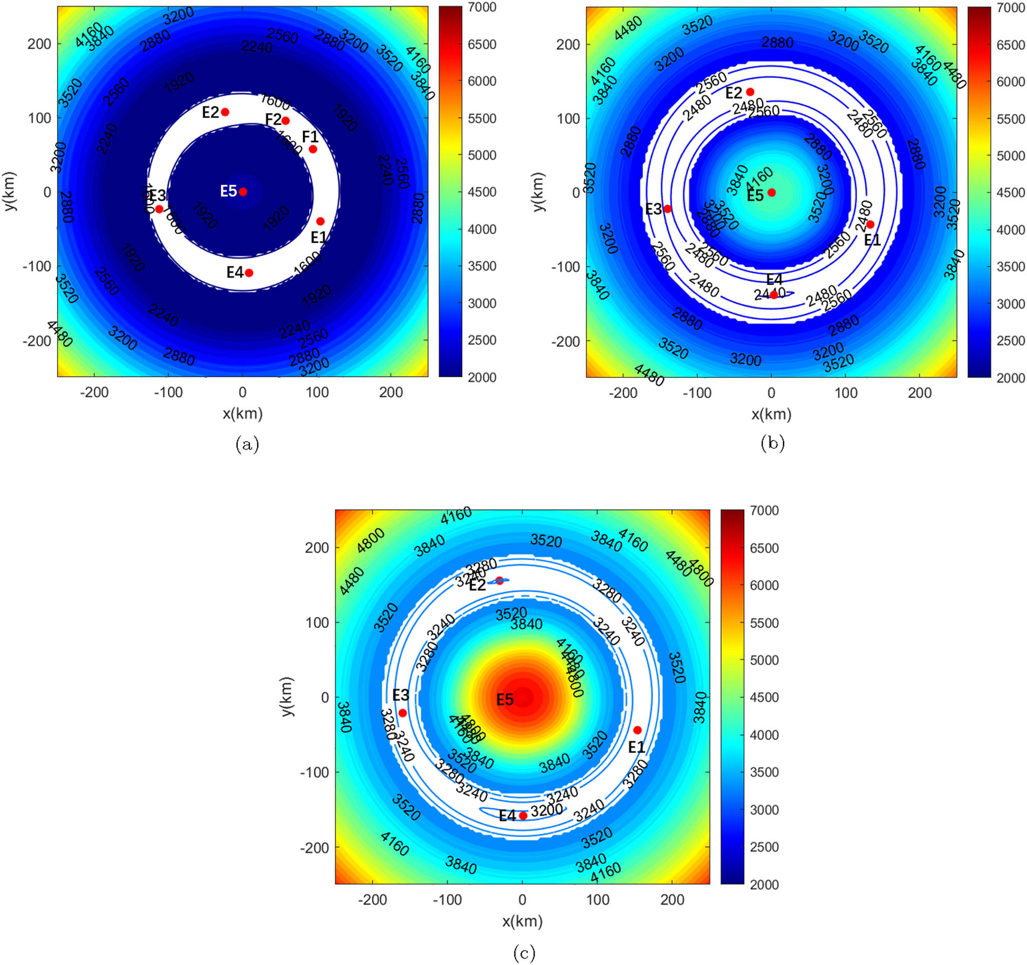
3.2 The change of density
Then, we considered the change of the equilibrium points during density changes and we defined the initial density
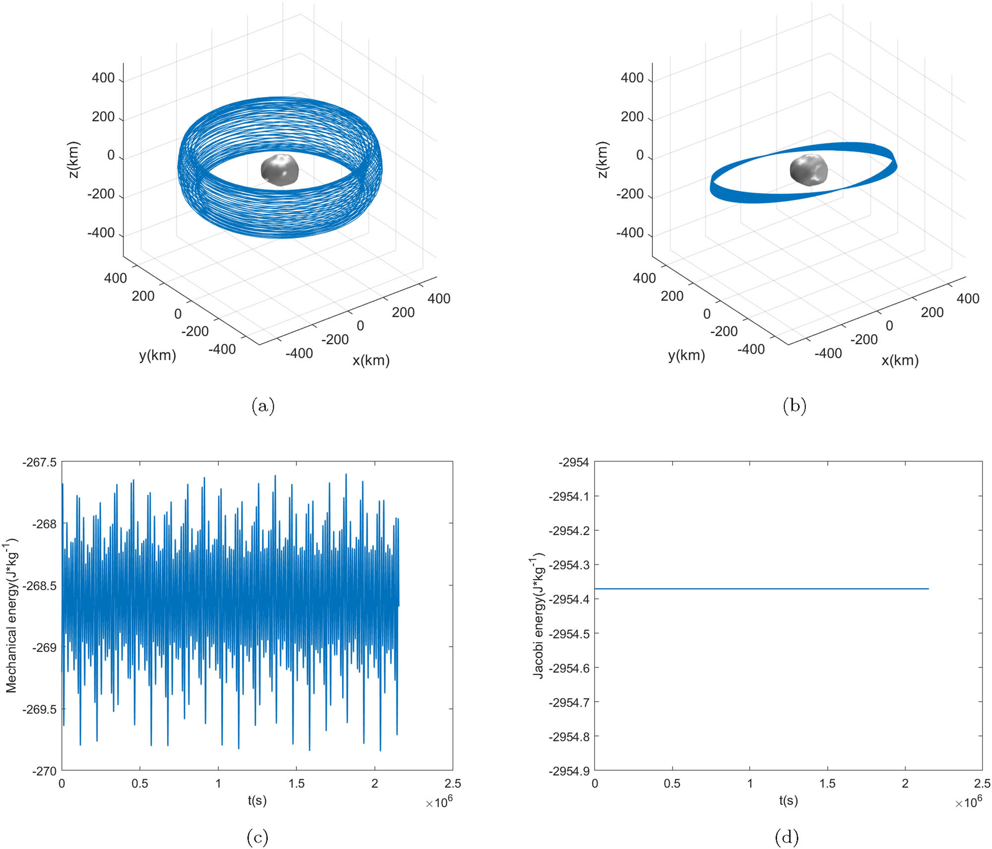
Orbit simulation of Minerva moonlet. (a) 3D map of the orbit in the body-fixed coordinate system. (b) 3D map of the orbit in the inertial system. (c) Mechanical energy of the orbit. (d) Jacobian integral of orbits.
Eigenvalues of the equilibrium points around Minerva when
| Equilibrium points |
|
|
|
|
|
|
|---|---|---|---|---|---|---|
| E1 |
|
|
|
|
0.000080 |
|
| E2 |
|
|
|
|
|
|
| E3 |
|
|
|
|
0.000097 |
|
| E4 |
|
|
|
|
|
|
| E5 |
|
|
|
|
|
|
Eigenvalues of the equilibrium points around Minerva when
| Equilibrium points |
|
|
|
|
|
|
|---|---|---|---|---|---|---|
| E1 |
|
|
|
|
0.000137 |
|
| E2 |
|
|
|
|
|
|
| E3 |
|
|
|
|
0.000174 |
|
| E4 |
|
|
|
|
|
|
| E5 |
|
|
|
|
0.000182 |
|
| F1 |
|
|
|
|
|
|
| F2 |
|
|
|
|
0.000137 |
|
Equilibrium points topological cases around Minerva at different densities
| Density | E1 | E2 | E3 | E4 | E5 | F1 | F2 |
|---|---|---|---|---|---|---|---|
|
|
Case 2 | Case 4a | Case 2 | Case 4a | Case 1 | Case 1 | Case 2 |
|
|
Case 2 | Case 1 | Case 2 | Case 1 | Case 1 | — | — |
|
|
Case 2 | Case 1 | Case 2 | Case 1 | Case 1 | — | — |
As shown in Figure 6 and Table 7 that when
4 Simulation of the moonlet orbits
Asteroid Minerva has two small moonlets: Aegis and Gorgoneion. Their semi-major axes of rotation around the primary asteroid are 623.5 and 375 km (Marchis et al. 2013). To understand the small moonlets motion under Minerva’s gravitational potential, we simulated the motion of Gorgoneion. Since Aegis is too far from Minerva, the motion of Gorgoneion is more meaningful to research.
Figure 7 shows the simulation of the Gorgoneion’s orbit under the Minerva gravitational potential. Figure 7(a) shows 3D maps of the orbits relative to the body-fixed coordinate system, and Figure 7(b) shows 3D maps of the orbits relative to the equatorial inertial coordinate system. At the initial moment of the orbit simulation, the position is located on the
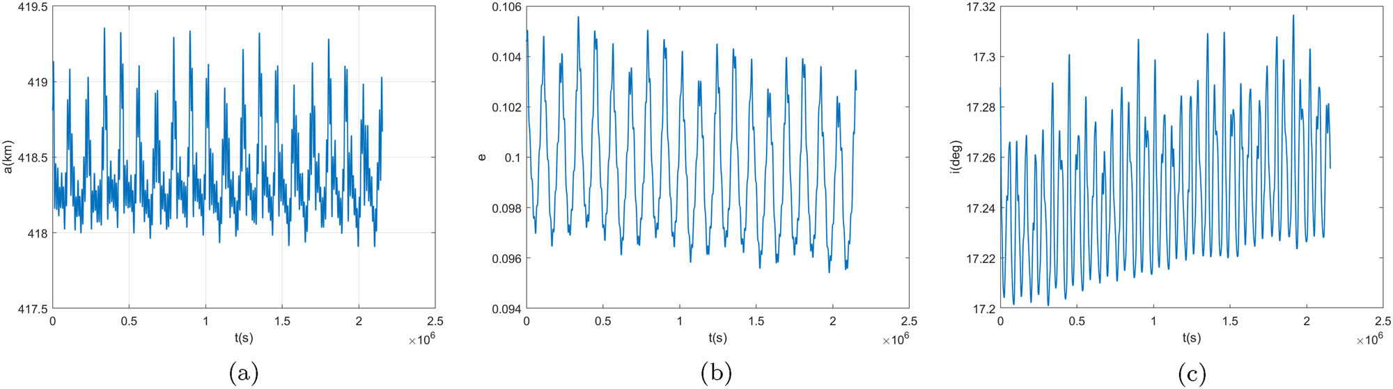
The orbital elements of simulation. (a) The semi-major axis. (b) The eccentricity. (c) The inclination of the orbit relative to the equatorial plane of Minerva.

Orbits around Minerva in different initial distances (
Our results show the existence of stable orbits in the gravitational potential of Minerva. When the orbit semi-major axis is the same as Gorgoneion and the eccentricity is about 0.1, then there will be at least one stable orbit exists around Minerva. Through the previous research, when the particle moves near the equilibrium points, the value of the effective potential will change significantly (Jiang 2018). We can see from the figure of effective potential shown in Section 2, it is relatively difficult to obtain a stable periodic orbit around the equilibrium points. Therefore, if we want the irregular shape of Minerva to have less perturbation to the particle’s orbit, the particle should move away from the equilibrium points. For Minerva, the four external equilibrium points are all located close to 150 km from the centroid of the asteroid. In Figure 9, we simulated the orbits at different initial distances, we can see that when the initial distance is 150 or 180 km, the orbits are unstable, but when the initial distance is 200 or 300 km the orbits are stable. So to maintain the stability of the orbits, the distance of the orbit relative to the centroid of the asteroid should be much more than 150 km.
5 Conclusion
In this article, we established a three-dimensional model of the asteroid 93 Minerva using the irregular shape model from observations. On the basis of this model, we calculated the physical size of asteroid Minerva to be
We studied the changing trend of equilibrium points by changing the spin speed and density of the Minerva. Keeping the density of Minerva constant and increasing its spin speed gradually and the number of equilibrium points will first increase from five to seven, then the annihilations occur, two equilibrium points collide and annihilate each other, the number of equilibrium points will decrease to one finally. When the spin speed is constant and the density changed, and
Acknowledgments
We gratefully acknowledge the reviewers for their helpful and constructive suggestions that helped us substantially improve the article.
-
Funding information: This work was supported by the Natural Science Foundation of China (No. U21B2050, No. 11902238) and the China Postdoctoral Science Foundation funded project (No. 2020M673373). All contributions by the co-author XiaoDuan Zou are not funded by NASA or any Chinese agency.
-
Author contributions: H.L.: conceptualization, methodology, software, validation, data curation, writing-original draft, visualization, and project administration; Y.J.: conceptualization, methodology, software, validation, supervision, project administration, and funding acquisition; A.L.: conceptualization, methodology, formal analysis, data curation, writing-original draft, supervision, and project administration; Y.W.: software, formal analysis, resources, writing-original draft, and visualization; X.Z.: writing-review and editing; J.P.: resources and writing-review and editing; Y.C.: formal analysis and writing-original draft; Y.Y.: resources and writing-review and editing; C.Z.: resources and writing-review and editing; Y.L.: resources and writing-review and editing; J.C.: resources and writing-review and editing.
-
Conflict of interest: The authors declare no conflict of interest.
Appendix
The detailed calculation of the equilibrium points eigenvalues.
The linearized equation of motion of the massless particle relative to the equilibrium point can be written as equation (A1). The characteristic equation of the equation (A4) could be satisfied as equation (A5). Through the calculation, we can obtain the eigenvalues of the equilibrium points.
In the aforementioned expression:
References
Abe S, Mukai T, Hirata N, Barnouin-Jha OS, Cheng AF, Demura H, et al. 2006. Mass and local topography measurements of Itokawa by Hayabusa. Science. 312(5778):1344–1347. 10.1126/science.1126272Suche in Google Scholar PubMed
Aljbaae S, Chanut TG, Prado AF, Carruba V, Hussmann H, Souchay J, et al. 2019. Orbital stability near the (87) Sylvia system. Mon Not R Astron Soc. 486(2):2557–2569. 10.1093/mnras/stz998Suche in Google Scholar
Barucci M, Fulchignoni M, Rossi A. 2007. Rosetta asteroid targets: 2867 Steins and 21 Lutetia. Space Sci Rev. 128(1):67–78. 10.1007/s11214-006-9029-6Suche in Google Scholar
Belton M, Veverka J, Thomas P, Helfenstein P, Simonelli D, Chapman C, et al. 1992. Galileo encounter with 951 Gaspra: First pictures of an asteroid. Science. 257(5077):1647–1652. 10.1126/science.257.5077.1647Suche in Google Scholar PubMed
Chanut T, Winter O, Amarante A, Araújo N. 2015. 3D plausible orbital stability close to asteroid (216) Kleopatra. Mon Not R Astron Soc. 452(2):1316–1327. 10.1093/mnras/stv1383Suche in Google Scholar
Fujiwara A, Kawaguchi J, Yeomans D, Abe M, Mukai T, Okada T, et al. 2006. The rubble-pile asteroid Itokawa as observed by Hayabusa. Science. 312(5778):1330–1334. 10.1126/science.1125841Suche in Google Scholar PubMed
Huang J, Ji J, Ye P, Wang X, Yan J, Meng L, et al. 2013. The ginger-shaped asteroid 4179 Toutatis: new observations from a successful flyby of changae-2. Sci Rep. 3(1):1–6. 10.1038/srep03411Suche in Google Scholar PubMed PubMed Central
Ji J, Jiang Y, Zhao Y, Wang S, Yu L. 2015. Chang’e-2 spacecraft observations of asteroid 4179 toutatis. Proc Int Astron Union. 10(S318):144–152. 10.1017/S1743921315008674Suche in Google Scholar
Jiang Y. 2015. Equilibrium points and periodic orbits in the vicinity of asteroids with an application to 216 Kleopatra. Earth, Moon, and Planets. 115(1):31–44.10.1007/s11038-015-9464-zSuche in Google Scholar
Jiang Y. 2018. Dynamical environment in the vicinity of asteroids with an application to 41 Daphne. Results Phys. 9:1511–1520. 10.1016/j.rinp.2018.05.001Suche in Google Scholar
Jiang Y. 2019. Dynamical environment in the triple asteroid system 87 Sylvia. Astrophys Space Sci. 364(4):1–12. 10.1007/s10509-019-3552-xSuche in Google Scholar
Jiang Y, Baoyin H. 2016. Periodic orbit families in the gravitational field of irregular-shaped bodies. Astron J. 152(5):137. 10.3847/0004-6256/152/5/137Suche in Google Scholar
Jiang Y, Baoyin H. 2018. Annihilation of relative equilibria in the gravitational field of irregular-shaped minor celestial bodies. Planet Space Sci. 161:107–136. 10.1016/j.pss.2018.06.017Suche in Google Scholar
Jiang Y, Baoyin H, Li H. 2015. Periodic motion near the surface of asteroids. Astrophys Space Sci. 360(2):1–10. 10.1007/s10509-015-2576-0Suche in Google Scholar
Jiang Y, Baoyin H, Li H. 2018. Orbital stability close to asteroid 624 Hektor using the polyhedral model. Adv Space Res. 61(5):1371–1385. 10.1016/j.asr.2017.12.011Suche in Google Scholar
Jiang Y, Baoyin H, Li J, Li H. 2014. Orbits and manifolds near the equilibrium points around a rotating asteroid. Astrophys Space Sci. 349(1):83–106. 10.1007/s10509-013-1618-8Suche in Google Scholar
Jiang Y, Baoyin H, Wang X, Yu Y, Li H, Peng C, et al. 2016. Order and chaos near equilibrium points in the potential of rotating highly irregular-shaped celestial bodies. Nonlinear Dyn. 83(1):231–252. 10.1007/s11071-015-2322-8Suche in Google Scholar
Jiang Y, Li H. 2019. Equilibria and orbits in the dynamical environment of asteroid 22 Kalliope. Open Astron. 28(1):154–164. 10.1515/astro-2019-0014Suche in Google Scholar
Jiang Y, Liu X. 2019. Equilibria and orbits around asteroid using the polyhedral model. New Astron. 69:8–20. 10.1016/j.newast.2018.11.007Suche in Google Scholar
Lazzaro D, Angeli C, Carvano J, Mothé-Diniz T, Duffard R, Florczak M. 2004. S3os2: The visible spectroscopic survey of 820 asteroids. Icarus. 172(1):179–220. 10.1016/j.icarus.2004.06.006Suche in Google Scholar
Marchis F, Descamps P, Hestroffer D, Berthier J, Vachier F, Boccaletti A, et al. 2003. A three-dimensional solution for the orbit of the asteroidal satellite of 22 Kalliope. Icarus. 165(1):112–120. 10.1016/S0019-1035(03)00195-7Suche in Google Scholar
Marchis F, Macomber B, Berthier J, Vachier F, Emery J. 2009. S/2009 (93) 1 and S/2009 (93) 2. Int Astron Union Circular. 9069:1. Suche in Google Scholar
Marchis F, Vachier F, Ďurech J, Enriquez J, Harris A, Dalba P, et al. 2013. Characteristics and large bulk density of the c-type main-belt triple asteroid (93) Minerva. Icarus. 224(1):178–191. 10.1016/j.icarus.2013.02.018Suche in Google Scholar
Mota ML, Rocco EM. 2019. Equilibrium points stability analysis for theasteroid 21 lutetia. In: Journal of Physics: Conference Series. Vol. 1365. IOP Publishing. p. 012007.10.1088/1742-6596/1365/1/012007Suche in Google Scholar
Moura T, Winter O, Amarante A, Sfair R, Borderes-Motta G, Valvano G. 2020. Dynamical environment and surface characteristics of asteroid (16) Psyche. Mon Not R Astron Soc. 491(3):3120–3136. 10.1093/mnras/stz3210Suche in Google Scholar
Price SD, Egan MP, Carey SJ, Mizuno DR, Kuchar TA. 2001. Midcourse space experiment survey of the galactic plane. Astron J. 121(5):2819. 10.1086/320404Suche in Google Scholar
Ryan EL, Woodward CE. 2010. Rectified asteroid albedos and diameters from iras and msx photometry catalogs. Astron J. 140(4):933. 10.1088/0004-6256/140/4/933Suche in Google Scholar
Scheeres DJ, Ostro SJ, Hudson R, Werner RA. 1996. Orbits close to asteroid 4769 Castalia. Icarus. 121(1):67–87. 10.1006/icar.1996.0072Suche in Google Scholar
Tedesco EF, Noah PV, Noah M, Price SD. 2002. The supplemental IRAS minor planet survey. Astron J. 123(2):1056. 10.1086/338320Suche in Google Scholar
Usui F, Kuroda D, Müller TG, Hasegawa S, Ishiguro M, Ootsubo T, et al. 2011. Asteroid catalog using AKARI: AKARI/IRC mid-infrared asteroid survey. Publ Astron Soc Jpn. 63(5):1117–1138. 10.1093/pasj/63.5.1117Suche in Google Scholar
Veverka J, Robinson M, Thomas P, Murchie S, Bell III J, Izenberg N, et al. 2000. NEAR at Eros Imaging and spectral results. Science. 289(5487):2088–2097. 10.1126/science.289.5487.2088Suche in Google Scholar PubMed
Veverka J, Thomas P, Harch A, Clark B, Bell III J, Carcich B, et al. 1997. NEAR’s flyby of 253 mathilde: Images of a C asteroid. Science. 278(5346):2109–2114. 10.1126/science.278.5346.2109Suche in Google Scholar PubMed
Wang X, Jiang Y, Gong S. 2014. Analysis of the potential field and equilibrium points of irregular-shaped minor celestial bodies. Astrophys Space Sci. 353(1):105–121. 10.1007/s10509-014-2022-8Suche in Google Scholar
Werner RA, Scheeres DJ. 1996. Exterior gravitation of a polyhedron derived and compared with harmonic and mascon gravitation representations of asteroid 4769 Castalia. Celest Mech Dyn Astron. 65(3):313–344. 10.1007/BF00053511Suche in Google Scholar
Yang B, Wahhaj Z, Beauvalet L, Marchis F, Dumas C, Marsset M, et al. 2016. Extreme ao observations of two triple asteroid systems with sphere. Astrophys J Lett. 820(2):L35. 10.3847/2041-8205/820/2/L35Suche in Google Scholar
Yu Y, Baoyin H. 2012a. Generating families of 3D periodic orbits about asteroids. Mon Not R Astron Soc. 427(1):872–881. 10.1111/j.1365-2966.2012.21963.xSuche in Google Scholar
Yu Y, Baoyin H. 2012b. Orbital dynamics in the vicinity of asteroid 216 Kleopatra. Astron J. 143(3):62. 10.1088/0004-6256/143/3/62Suche in Google Scholar
Zhao Y, Wang S, Hu S, Ji J. 2013. A research on imaging strategy and imaging simulation of toutatis in the Chang’e 2 flyby mission. Acta Astron Sin. 54(5):447–454. Suche in Google Scholar
Zou X, Li C, Liu J, Wang W, Li H, Ping J. 2014. The preliminary analysis of the 4179 Toutatis snapshots of the Changae-2 flyby. Icarus. 229:348–354. 10.1016/j.icarus.2013.11.002Suche in Google Scholar
© 2022 Hu Liu et al., published by De Gruyter
This work is licensed under the Creative Commons Attribution 4.0 International License.
Artikel in diesem Heft
- Research Articles
- Deep learning application for stellar parameters determination: I-constraining the hyperparameters
- Explaining the cuspy dark matter halos by the Landau–Ginzburg theory
- The evolution of time-dependent Λ and G in multi-fluid Bianchi type-I cosmological models
- Observational data and orbits of the comets discovered at the Vilnius Observatory in 1980–2006 and the case of the comet 322P
- Special Issue: Modern Stellar Astronomy
- Determination of the degree of star concentration in globular clusters based on space observation data
- Can local inhomogeneity of the Universe explain the accelerating expansion?
- Processing and visualisation of a series of monochromatic images of regions of the Sun
- 11-year dynamics of coronal hole and sunspot areas
- Investigation of the mechanism of a solar flare by means of MHD simulations above the active region in real scale of time: The choice of parameters and the appearance of a flare situation
- Comparing results of real-scale time MHD modeling with observational data for first flare M 1.9 in AR 10365
- Modeling of large-scale disk perturbation eclipses of UX Ori stars with the puffed-up inner disks
- A numerical approach to model chemistry of complex organic molecules in a protoplanetary disk
- Small-scale sectorial perturbation modes against the background of a pulsating model of disk-like self-gravitating systems
- Hα emission from gaseous structures above galactic discs
- Parameterization of long-period eclipsing binaries
- Chemical composition and ages of four globular clusters in M31 from the analysis of their integrated-light spectra
- Dynamics of magnetic flux tubes in accretion disks of Herbig Ae/Be stars
- Checking the possibility of determining the relative orbits of stars rotating around the center body of the Galaxy
- Photometry and kinematics of extragalactic star-forming complexes
- New triple-mode high-amplitude Delta Scuti variables
- Bubbles and OB associations
- Peculiarities of radio emission from new pulsars at 111 MHz
- Influence of the magnetic field on the formation of protostellar disks
- The specifics of pulsar radio emission
- Wide binary stars with non-coeval components
- Special Issue: The Global Space Exploration Conference (GLEX) 2021
- ANALOG-1 ISS – The first part of an analogue mission to guide ESA’s robotic moon exploration efforts
- Lunar PNT system concept and simulation results
- Special Issue: New Progress in Astrodynamics Applications - Part I
- Message from the Guest Editor of the Special Issue on New Progress in Astrodynamics Applications
- Research on real-time reachability evaluation for reentry vehicles based on fuzzy learning
- Application of cloud computing key technology in aerospace TT&C
- Improvement of orbit prediction accuracy using extreme gradient boosting and principal component analysis
- End-of-discharge prediction for satellite lithium-ion battery based on evidential reasoning rule
- High-altitude satellites range scheduling for urgent request utilizing reinforcement learning
- Performance of dual one-way measurements and precise orbit determination for BDS via inter-satellite link
- Angular acceleration compensation guidance law for passive homing missiles
- Research progress on the effects of microgravity and space radiation on astronauts’ health and nursing measures
- A micro/nano joint satellite design of high maneuverability for space debris removal
- Optimization of satellite resource scheduling under regional target coverage conditions
- Research on fault detection and principal component analysis for spacecraft feature extraction based on kernel methods
- On-board BDS dynamic filtering ballistic determination and precision evaluation
- High-speed inter-satellite link construction technology for navigation constellation oriented to engineering practice
- Integrated design of ranging and DOR signal for China's deep space navigation
- Close-range leader–follower flight control technology for near-circular low-orbit satellites
- Analysis of the equilibrium points and orbits stability for the asteroid 93 Minerva
- Access once encountered TT&C mode based on space–air–ground integration network
- Cooperative capture trajectory optimization of multi-space robots using an improved multi-objective fruit fly algorithm