The evolution of time-dependent Λ and G in multi-fluid Bianchi type-I cosmological models

Alnadhief H. A. Alfedeel; Amare Abebe

doi:10.1515/astro-2022-0027

Artikel Open Access

The evolution of time-dependent Λ and G in multi-fluid Bianchi type-I cosmological models

Alnadhief H. A. Alfedeel und Amare Abebe

Veröffentlicht/Copyright: 24. Mai 2022

Veröffentlicht von

Veröffentlichen auch Sie bei De Gruyter Brill

Manuskript einreichen Informationen für Autor*innen Erkunden Sie dieses Fachgebiet

Aus der Zeitschrift Open Astronomy Band 31 Heft 1

Abstract

In this work, cosmological solutions based on the time-dependent cosmological ( Λ ) and Newtonian ( G ) running “constants” in the Bianchi type-I spacetime are investigated vis-à-vis known cosmological data. The observationally known values of Ω m , Ω r and Ω Λ have been used to solve the Einstein field equations for the model and the resulting behaviours of the physical and dynamical quantities, with particular emphasis on late-time cosmology, are discussed. Our analysis indicates that certain choices of the defining model parameters give results consistent with the observed behaviour of the universe, such as accelerated expansion and an early anisotropy that vanishes at late times.

Keywords: Bianchi metric; anisotropic; varying Λ; varying G

PACS 2020: 04.20.-q; 04.50.Kd; 99.80-k; 98.80-Jk

1 Introduction

Recent cosmological observations have shown that the universe in conformity with the cosmological principle, i.e., it is almost homogeneous and isotropic on large scales. Moreover, it is undergoing a recent epoch of accelerated expansion. Although it is not conclusively known what caused this recent cosmic acceleration, the prevailing argument is that dark energy caused it.

Among the most widely considered candidates of dark energy is the vacuum energy of the cosmological constant Λ . But there are some serious problems associated with the cosmological constant, among them the eponymous cosmological constant problem (Weinberg 1989) and the coincidence problem (Velten et al. 2014). These are serious problems that cannot be ignored, and several alternatives to the vacuum energy solution are being thought currently.

Dirac’s hypothesis that the gravitational constant decreases with time has been a matter of scrutiny for some time (Canuto et al. 1979), but recent attempts to consider both Λ and the universal gravitational constant G as dynamical quantities, and therefore not as constants, have gained more attention due to the aforementioned not-so-well-explained cosmic acceleration.

Since the isotropy assumption is only an approximation on large scales, and not something explained from first principles, there is the possibility that the spatially homogeneous and anisotropic cosmological modes play a significant role in explaining the evolution of the universe at its early stages. At these times, the universe was full of anisotropies with a highly irregular mechanism that isotropised later. In fact, several authors have shown over the years that there is some degree of anisotropy in the observed universe that necessitates the consideration of a non-FLRW geometry (see, e.g., Misner 1968, Pereira et al. 2007, Almeida et al. 2022). Hence, there is a need for a detailed study of cosmological models that describe an early-time anisotropy with a proper mechanism to produce [near] isotropy at late times on the one hand and an accelerated expansion at the present epoch on the other hand.

In view of the aforementioned motivation, various researchers have investigated the anisotropic Bianchi type cosmological models with variable forms of G and Λ and different types of fluids (Singh and Tiwari 2008, Singh et al. 2008, Singh and Singh 2012, Arbab 1998, Pradhan and Kumar 2001, Pradhan and Ostarod 2006, Mazumder 1994, Tiwari 2008, Dwivedi 2012, Yadav 2013). For instance, Einstein equations for Bianchi type-I cosmological model, a self-consistent system of interacting spinor and scalar fields with isotropic distribution of matter, was first obtained by Saha and Shikin (1997) and further developed by Saha (2001b). Saha (2001a) earlier considered an analogous study of a self-consistent nonlinear spinor field and Bianchi type-I gravitational one with time-dependent gravitational constant G and cosmological constant Λ . Furthermore, Belinskii (1975) examined the Bianchi type-I model with a viscous fluid to study the nature of cosmological solutions. According to their conclusions, “the viscosity can cause new qualitative behaviour of the solution close to the singularity.” Furthermore, Banerjee et al. (1985) studied the Bianchi type-I cosmological model with the shear viscosity having a power-law function of energy density ρ for a stiff perfect fluid. Likewise, Singh et al. (2014) investigated Bianchi type-I cosmological models with time-varying Λ for viscous-fluid distributions. They obtained an exact solution for Einstein’s field equations (EFEs) by assuming the expansion anisotropy A p to be a spatial volume function. Moreover, they noted that the cosmological constant Λ asymptotically decays with time, and the universe in this model becomes isotropic at future (late) times. In addition, Mak and Harko (2002) considered a flat Bianchi type-I space-time with a constant positive deceleration parameter q to examine the dynamics of a causal bulk viscous-fluid universe. One of the current authors recently investigated (Alfedeel 2020) the homogeneous and anisotropic Bianchi type-I cosmological model with a time-varying ( Λ = α S − 2 + β H 2 ) cosmological and Newtonian’s constants and obtained the most generalised analytical solutions to the EFEs for a Zeldovich (stiff-fluid) Bianchi type-I cosmological model without assuming any coupling relationship between the metric variables or making any prior choice in the numerical values α and β that appear on the Λ term. It was shown that the solution for the average scale factor for the generalised Friedman equation involves the hyper-geometric function. The majority of previous studies of Bianchi type I and V cosmological models describe an expanding, shearing, non-rotating, and transient universe, which was decelerating at early periods and accelerating at the present epoch.

The main purpose of this article, as a follow-up of the aforementioned work (Alfedeel 2020), is to reformulate the reduced system of differential equations (DEs) of the Einstein field equations for Bianchi type-I cosmology model with time-dependent G and Λ in terms of the constrained parameters Ω m , Ω r , and Ω Λ from the recent observational data of H ( z ) , SNeIa, and BAO, and then use the numerical integration methods (Runge–Kutta fourth order) to solve these DEs simultaneously. The rest of this article is structured as follows: In Section 2, we display the background spacetime and cosmology of the Bianchi type-I model and its solutions. Section 3 presents our results and discussions. We then conclude with the main results of this article in Section 4.

2 Bianchi type-I cosmology

The line-element of the spatially homogeneous and anisotropic Bianchi type- I , which measures the distance between two points in space, is given by:

(1) d s 2 = − d t 2 + A 2 ( t ) d x 2 + B 2 ( t ) d y 2 + C 2 ( t ) d z 2 ,

where A ( t ) , B ( t ) , and C ( t ) are the scale factors along x , y , and z direction. The perfect-fluid cosmic matter distribution is given by the following energy-momentum tensor:

(2) T i j = ( p + ρ ) u i u j + p g i j ,

where ρ is the matter density, u i = δ t i = ( − 1 , 0 , 0 , 0 ) is the normalised fluid four velocity, which is a time-like quantity such that u i u i = − 1 , and p is the fluid’s isotropic pressure that is related to mater density through the barotropic equation of state (EoS) p = w ρ , with

w = 0 for dust , 1 / 3 for radiation , − 1 for dark energy .

The Einstein field equations with time-dependent Λ = α S 2 + β H 2 , where S = ( ABC ) 1 / 3 is the average scale factor, H is the average Hubble parameter, and G = G ( t ) and the conservation of the usual energy-momentum tensor T i j (i.e., ∇ j T i j = 0 ) are reduced to the energy density evolution (Alfedeel 2020).

(3) ρ ˙ + ( ρ + p ) A ˙ A + B ˙ B + C ˙ C = 0 ,

giving a solution for the energy density as follows:

(4) ρ = ρ 0 S 3 ( 1 + w ) ,

where ρ 0 corresponds to the current value of the energy density. The generalised Friedmann equations read:

(5) 8 π G p − Λ = ( 2 q − 1 ) H 2 − σ 2 ,

(6) 8 π G ρ + Λ = 3 H 2 − σ 2 ,

where σ is the shear modules and q is the deceleration parameter. Or alternatively

(7) S ¨ S + ( 2 − β ) S ˙ 2 S 2 − α S 2 = 4 π G ( t ) ( ρ − p ) .

In the multi-fluid setting, ρ and p are the total energy density and total pressure of the cosmic fluid, respectively. The time evolution equation connecting G and Λ can be given by

(8) 8 π ρ G ˙ + Λ ˙ = 0 ,

and the expression for the metric variables A , B , and C as follows:

(9) A = A 0 S exp k 1 ∫ d t S 3 ,

(10) B = B 0 S exp k 2 ∫ d t S 3 ,

(11) C = C 0 S exp k 3 ∫ d t S 3 ,

where m 1 , m 2 , m 3 , k 1 , k 2 , k 3 , and x 1 , x 2 , and x 3 are constants of integration (Singh and Kumar 2009) satisfying the following relations:

(12) A 0 = m 1 m 2 3 , B 0 = m 1 − 1 m 3 3 , C 0 = ( m 1 m 3 ) − 1 3 , k 1 = 2 x 1 + x 3 3 , k 2 = x 3 − x 1 3 , k 3 = − x 1 + 2 x 3 3 , A 0 B 0 C 0 = 1 , k 1 + k 2 + k 3 = 0 .

It is worth mentioning that solutions (9)–(11) were first obtained by Saha and Shikin (1997) and Saha (2001b). In this model, the physical and dynamical parameters, the deceleration parameter q , the average anisotropy parameter A p , and shear module σ are defined as in the studies by Alfedeel et al. (2018) and Carvalho et al. (1992) by:

(13) q = − S ¨ S S ˙ 2 = − 1 − H ˙ H 2 ,

(14) A p = 1 3 ∑ i = 1 3 H i − H H 2 ,

(15) σ 2 = 1 3 A ˙ 2 A 2 + B ˙ 2 B 2 + C ˙ 2 C 2 − 1 3 A ˙ B ˙ A B + B ˙ C ˙ B C + A ˙ C ˙ A C = 1 2 A ˙ 2 A 2 + B ˙ 2 B 2 + C ˙ 2 C 2 − 3 H 2 2 ⇒ σ = K S 3 ,

where K = ( x 1 2 + x 2 2 + x 1 x 2 ) / 3 is a numerical constant, which is related to the anisotropy of the model. We see that the Bianchi type- I model is fully characterised by the set of several parameters H , σ , G Λ , and q ; the metric variables A , B , and C ; and the energy density ρ , but the system is not complete until the value of the average scale factor S ( t ) is known.

2.1 Model from data

Throughout this section, the constrained density parameters (Farooq and Ratra 2013) Ω m , Ω r , and Ω Λ from the recent observational data will be used to study the evolution of time-dependent Λ and G Bianchi type-I cosmological models. To proceed, we need to rewrite the reduced differential equations (DEs) in Section 2 in terms of the density parameter Ω . Therefore, we may introduce

(16) ρ i0 = 3 H 0 2 8 π G 0 Ω i0 ⇒ ρ i = 3 H 0 2 8 π G 0 Ω i0 ( 1 + z ) ( 1 + w )

as the mass density of the universe components, where H 0 is the current value of the Hubble parameter, G 0 = 6.67 × 1 0 − 1 Nm 2 kg − 2 is the Newtonian constant at t 0 – taken here to correspond to the present time – and Ω i is the fractional density parameter of the ith component of the multi-fluid system filling the universe.

2.2 The numerical solution

Having introduced the defining parameters for the Bianchi-I model, we can obtain the following set of non-linear first-order differential equations that describe the evolution of the background:

(17) d S d t = Z ,

(18) d Z d t = − ( 2 − β ) Z 2 S + α S + c 1 S G ,

(19) d G d t = c 2 Z S 3 + c 3 Z 3 S 3 − c 4 Z S 2 G ,

where we have used the following short hands:

c 1 ≡ 3 H 0 2 2 G 0 Ω mo ( 1 + z ) 3 + 2 Ω r0 3 ( 1 + z ) 4 + 2 Ω Λ 0 , c 2 ≡ 2 α ( 1 − β ) G 0 3 H 0 2 , c 3 ≡ 2 β ( 3 − β ) G 0 3 H 0 2 , c 4 ≡ β Ω mo ( 1 + z ) 3 + 2 Ω r0 3 ( 1 + z ) 4 + 2 Ω Λ 0 .

These are numerical constants that totally depend on the value of α , β , and G 0 and the measurements of H 0 , Ω m0 , Ω r0 , and Ω Λ 0 from the data survey. Note that we have assumed flat space, and hence, Ω m0 + Ω r0 + Ω Λ 0 = 1 by definition.

2.3 Equations in redshift space

To transform the background evolution equations, i.e., the underlying Bianchi type-I system of DEs, any time dependent quantity Q will be transformed into redshift as follows:

d Q d t = d Q d z d z d a d a d t = a H d z d a d Q d z ,

where

a ( z ) = 1 1 + z , d z d a = − ( 1 + z ) 2 .

Thus, using these definitions, Eqs. (18) and (19) can be transformed into redshift space as follows:

(20) d H d z = ( 3 − β ) ( 1 + z ) H − α ( 1 + z ) H − c 1 G ( 1 + z ) H ,

(21) d G d z = − c 2 ( 1 + z ) − c 3 H 2 ( 1 + z ) + c 4 G .

These two equations describe an equivalent dynamical system as the one described by Eqs. (17), (18), and (19). For the sake of computational suitability, let us now define the dimensionless parameters corresponding to the defining dimensional parameters of the model as follows:

h ≡ H H 0 , λ ≡ Λ Λ 0 , g ≡ G G 0 , γ ≡ α H 0 2 .

In these parameters, our previous equations can be re-written in a fully dimensionless form as follows:

(22) d h d z = ( 3 − β ) ( 1 + z ) h − γ ( 1 + z ) h − 3 2 g ( 1 + z ) h × Ω mo ( 1 + z ) 3 + 2 Ω r0 3 ( 1 + z ) 4 + 2 Ω Λ 0 ,

(23) d g d z = β Ω mo ( 1 + z ) 3 + 2 Ω r0 3 ( 1 + z ) 4 + 2 Ω Λ 0 g − 2 β 3 ( 3 − β ) h 2 1 + z − 2 γ 3 ( 1 − β ) ( 1 + z ) .

Once we have calculated h and g , we can use it to obtain the deceleration parameters:

(24) q = ( 2 − β ) − γ ( 1 + z ) 2 h 2 − 3 2 Ω mo ( 1 + z ) 3 + 2 Ω r0 3 ( 1 + z ) 4 + 2 Ω Λ 0 g h 2

as well as the scale factor solutions of the model

(25) A = A 0 ( 1 + z ) exp κ 1 ∫ ( 1 + z ) 2 d z h ,

(26) B = B 0 ( 1 + z ) exp κ 2 ∫ ( 1 + z ) 2 d z h ,

(27) C = C 0 ( 1 + z ) exp κ 3 ∫ ( 1 + z ) 2 d z h ,

where we have defined the new dimensionless parameters κ 1 ≡ k 1 / H 0 , κ 2 ≡ k 2 / H 0 , and κ 3 ≡ k 3 / H 0 . In the following, we plot the numerical values of A p , G / G 0 , Λ / Λ 0 , σ , h , and q using Ω m0 = 0.3111 ± 0.0056 , Ω Λ 0 = 0.6889 ± 0.0056 , Ω r0 = 1 − Ω m0 − Ω Λ 0 , and H 0 = 67.37 ± 0.54 km/s/Mpc (Aghanim et al. 2008). The DEs are integrated with respect to redshift z with initial conditions h ( 0 ) = g ( 0 ) = 1 , and β = 0.02 using the fourth-order Runge–Kutta numerical integration method.

3 Results and discussion

The observed and currently accepted values of Ω m0 , Ω r0 , Ω Λ 0 , H 0 , and G 0 are used to numerically solve the coupled system of first-order differential equations, i.e., Eqs. (22)–(23) for a multi-component cosmological fluid along with the normalised initial conditions h ( 0 ) = g ( 0 ) = 1 using the fourth-order Runge–Kutta computational method. The numerical results were obtained for several values of γ in the range [ − 0.006 , 0.006 ] and for β = 0.02 . The effect of the re-scaled parameter γ on the behaviour of λ , g , h , q , σ , and A p is graphically represented in Figures 1, 2, 3, 4, 5, 6 that follow.

$Figure 1 The variation of Λ \Lambda in redshift, as normalised by the value of Λ 0 {\Lambda }_{0} today.$

Figure 1

The variation of Λ in redshift, as normalised by the value of Λ 0 today.

$Figure 2 The variation h h in redshift, as normalised by the value of H 0 {H}_{0} today.$

Figure 2

The variation h in redshift, as normalised by the value of H 0 today.

$Figure 3 The variation G G in redshift, as normalised by the value of G 0 {G}_{0} today.$

Figure 3

The variation G in redshift, as normalised by the value of G 0 today.

Figure 4

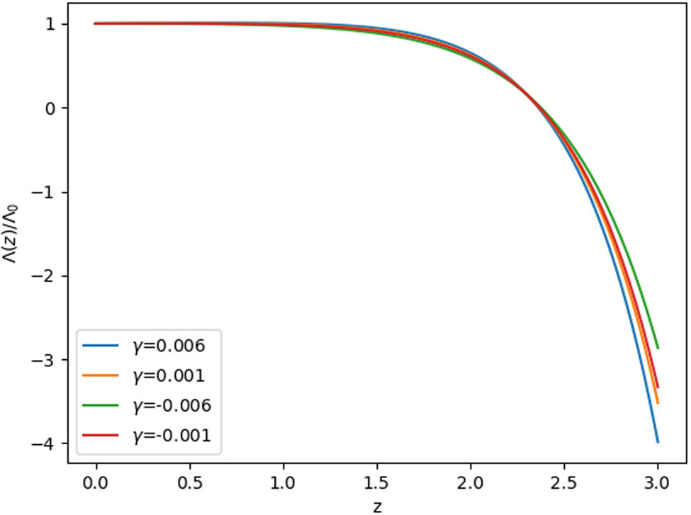
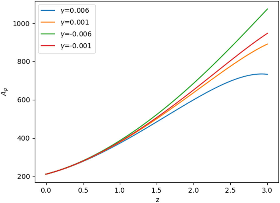
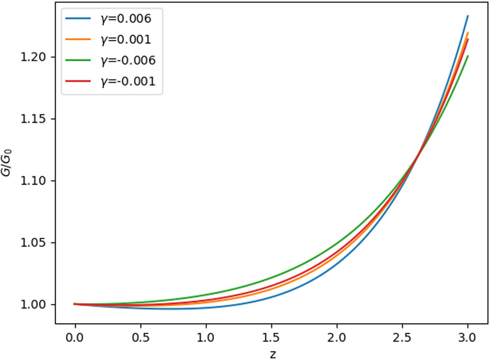
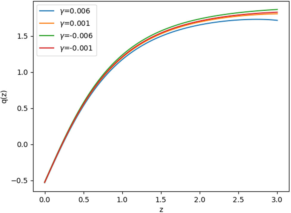
The variation of the deceleration parameter in redshift.

Figure 5

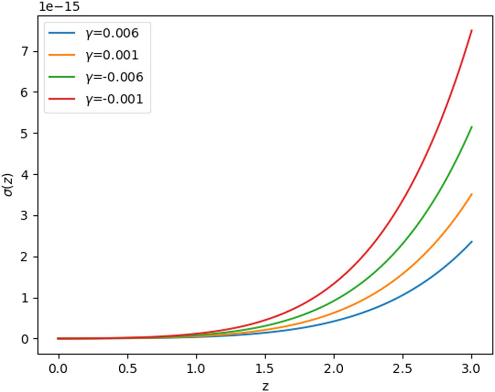
The evolution of the shear parameter in redshift.

Figure 6

The evolution of the anisotropy parameter in redshift.

From these figures, the plots for λ and g show that, as could be predicted from Eq. (8), Λ and G evolve in opposite trends: for values of the parameter γ for which G decreases with time (increases with redshift), Λ increases with time (decreases with redshift), and vice versa. Importantly, Figure 1 shows that Λ becomes significant today, which is in accordance with the late-time domination of the universe by dark energy. It is only interesting to note that it could have negative values in the past. In other words, the cosmological parameter Λ as one of the potential candidates for dark energy fits well into this description of dark energy dominating at the present time, but could have been dominated by other component fluids in the cosmological past. Similarly, one can think of Figure 2 as implying that because gravity is weaker today than in the past, an acceleration in the expansion is expected at late times. That is, since gravity is not be strong enough to keep bound structures, like galaxies, clusters, and superclusters together, the spacetime between these structures expands faster. These two results naturally complement each other, as depicted by Eq. (8). Another observation worth mentioning is the fact that at about redshift of z ∼ 2.5 , the ordering of the magnitudes of Λ and G changes as one varies the α parameter. We also note that each of H , σ , and A p parameters are decreasing functions of redshift for the different values of α considered. This is also consistent with observations as, for example, one has a more or less isotropic universe on large scales today but suggestions of more anisotropy in the past.

The plots of the deceleration parameter q show that for appropriate values of γ considered, positive q values in the past and negative q values in recent epochs – from a redshift of z ∼ 0.5 to about now – can be achieved, in agreement with observational data. Importantly, it is easy to see from the figure that q takes present-day values of slightly below − 0.5 for the parameter space of the model we considered.

4 Conclusion

In this work, we have found generic solutions for the Bianchi type-I cosmological model with time-varying Newtonian and cosmological “constants” for realistic multi-component perfect-fluid scenarios. In the solution process, we rewrote the EFEs for the specific model of our interest as a closed system of two first-order differential equations involving normalised and dimensionless cosmological parameters g ( z ) and h ( z ) in redshift space. We then integrated this system numerically using the fourth-order Runge–Kutta method and by inputting the observationally known values of the fractional energy densities today, as well as setting the initial condition today, with the normalised values of g ( z = 0 ) = 1 and h ( z = 0 ) = 1 today, by definition.

The predicted evolution of the different cosmological parameters for the Bianchi- I spacetimes endowed with multi-component fluids is depicted in Figures 1–6. Figure 3 shows that for each value of the defining parameter α in Λ = α S − 2 + β H 2 (redefined as the dimensionless parameter γ for the plotting), the Newtonian gravitational factor G decreases with time as Dirac would have it, and as can be predicted from the nature of Eq. (8), the opposite effect is observed for the evolution of Λ , the interesting aspect being both of them asymptoting towards constant values today. The results can help to rule out some values of the model parameters if we accurately know the observational values (and signs) of Λ and G throughout the cosmological evolution. Figure 2 shows that the larger value of α , the smaller the value of the Hubble parameter, whereas all values of α produce accelerated expansion ( q < 0 ) at late times. Figure 6 shows that even if we start with some anisotropic universe in the past, we will have an isotropic universe at late times, possibly indistinguishable from the FLRW universe. It is worth further exploring this last aspect, as well as putting more stringent constraints on the values of the defining parameters of the model, with more rigorous data and statistical analysis – using existing and upcoming cosmological data– including large-scale structure formation scenarios. This is a task we will come back to in the near future.

Acknowledgments

The authors extend their appreciation to the Deanship of Scientific Research at Imam Mohammad Ibn Saud Islamic University for funding this work through Research Group no. RG-21-09-18.

Author contributions: All authors have accepted responsibility for the entire content of this manuscript and approved its submission.
Conflict of interest: The authors state no conflict of interest.

References

Aghanim N, Akrami Y, Ashdown M, Aumont J, Baccigalupi C, Ballardini M, et al. 2008. Planck 2018 results-VI. Cosmological parameters. Astron Astrophys. 641:A6. 10.1051/0004-6361/201833910Suche in Google Scholar

Alfedeel AHA, Abebe A, Gubara HM. 2018. A generalised solutions of Bianchi type-V cosmological models with time dependent G and Λ. Universe. 4(8):83. 10.3390/universe4080083Suche in Google Scholar

Alfedeel AHA. 2020. Bianchi type-I model with time varying Λ and G: The generalised solution. Open Astron. 29(1):89–93. 10.1515/astro-2020-0012Suche in Google Scholar

Almeida JPB, Motoa-Manzano J, Noreña J, Pereira TS, Valenzuela-Toledo CA. 2022. Structure formation in an anisotropic universe: Eulerian perturbation theory. J Cosmol Astroparticle Phys. 2022(02):018. 10.1088/1475-7516/2022/02/018Suche in Google Scholar

Arbab IA. 1998. Bianchi type-I viscous universe with variable G and Lambda. Gen Relativ Gravit. 30(9):1401–1405. 10.1023/A:1018856625508Suche in Google Scholar

Banerjee JP, Duttachoudhuryi SB, Sanyal AK. 1985. Bianchi type-I cosmological model with a viscous fluid. J Math Phys. 26(11):3010–3015. 10.1063/1.526676Suche in Google Scholar

Belinskii VA. 1975. On influence of viscosity on the character of cosmological evolution. Zh Eksp Teor Fiz. 69:401–413. Suche in Google Scholar

Canuto V, Hsieh SH, Owen JR. 1979. Varying G. Mon Not R Astron Soc. 188(4):829. 10.1093/mnras/188.4.829Suche in Google Scholar

Carvalho JC, Lima JAS, Waga I. 1992. Cosmological consequences of a time-dependent Λ term. Phys Rev D. 46(6):2404. 10.1103/PhysRevD.46.2404Suche in Google Scholar

Dwivedi UK. 2012. Bianchi type-V models with decaying cosmological term Λ. Int J Management IT Eng. 2(7):568–573. Suche in Google Scholar

Farooq O, Ratra B. 2013. Hubble parameter measurement constraints on the cosmological deceleration-acceleration transition redshift. Astrophys J Lett. 766(1):7. 10.1088/2041-8205/766/1/L7Suche in Google Scholar

Mak MK, Harko T. 2002. Bianchi type-I universes with causal bulk viscous cosmological fluid. Int J Mod Phys D. 11(03):447–462. 10.1142/S0218271802001743Suche in Google Scholar

Mazumder A. 1994. Solutions of LRS Bianchi I space-time filled with a perfect fluid. Gen Relativ Gravit. 26(3):307–310. 10.1007/BF02108011Suche in Google Scholar

Misner CW. 1968. The isotropy of the universe. Astrophys J. 151:431. 10.1086/149448Suche in Google Scholar

Pereira TS, Pitrou C, Uzan JP. 2007. Theory of cosmological perturbations in an anisotropic universe. J Cosmol Astroparticle Phys. 09:006. 10.1088/1475-7516/2007/09/006Suche in Google Scholar

Pradhan A, Kumar A. 2001. LRS Bianchi I cosmological universe models with varying cosmological term Λ. Int J Mod Phys D. 10(03):291–298. 10.1142/S0218271801000718Suche in Google Scholar

Pradhan A, Ostarod S. 2006. Universe with time dependent deceleration parameter and Λ term in general relativity. Astrophys Space Sci. 306(1):11–16. 10.1007/s10509-006-9178-9Suche in Google Scholar

Pradhan A, Yadav L, Yadav AK. 2004. Viscous fluid cosmological models in LRS Bianchi type-V universe with varying Λ. Czech J Phys. 54(4):487–498. 10.1023/B:CJOP.0000020586.43735.b5Suche in Google Scholar

Saha B, Shikin GN. 1997. Interacting spinor and scalar fields in Bianchi type-I universe filled with perfect fluid: exact self-consistent solutions. Gen Relativ Gravit. 29(9):1099–1113. 10.1023/A:1018887024268Suche in Google Scholar

Saha B. 2001a. Dirac spinor in Bianchi-I universe with time-dependent gravitational and cosmological constants. Modern Phys Lett A. 16(20):1287–1296. 10.1142/S0217732301004546Suche in Google Scholar

Saha B. 2001b. Spinor field in a Bianchi type-I universe: regular solutions. Phys Rev D. 64(12):123501. 10.1103/PhysRevD.64.123501Suche in Google Scholar

Singh CP, Kumar S. 2009. Bianchi-I space-time with variable gravitational and cosmological constants. Int J Theor Phys. 48(8):2401–2411. 10.1007/s10773-009-0030-1Suche in Google Scholar

Singh PS, Singh JP. 2012. Bianchi type-V universe with bulk Viscous matter and time varying gravitational and cosmological constant. Res Astron Astrophys. 12:1457–1466. 10.1088/1674-4527/12/11/001Suche in Google Scholar

Singh JP, Tiwari RK. 2008. Perfect fluid Bianchi type-I cosmological models with time varying G and Λ. Pramana-J Phys. 70(4):565–574. 10.1007/s12043-008-0019-ySuche in Google Scholar

Singh CP, Ram S, Zeyauddin M. 2008. Bianchi type-V perfect fluid space-time models in general relativity. Astrophys Space Sci. 315(1):181–189. 10.1007/s10509-008-9811-xSuche in Google Scholar

Singh JP, Baghel PS, Singh A. 2014. Bianchi type-I cosmological models with viscous fluid and decaying vacuum. Prespacetime J. 5(8):785–803. Suche in Google Scholar

Tiwari RK. 2008. Bianchi type-I cosmological models with time dependent G and Λ. Astrophys Space Sci. 318(3):243–247. 10.1007/s10509-008-9924-2Suche in Google Scholar

Velten HE, Vom Marttens RF, Zimdahl W. 2014. Aspects of the cosmological coincidence problem. Eur Phys J C. 74(11):1–8. 10.1140/epjc/s10052-014-3160-4Suche in Google Scholar

Weinberg S. 1989. The cosmological constant problem. Rev Mod Phys. 61(1):1. 10.1007/978-3-662-04587-9_2Suche in Google Scholar

Yadav AK. 2013. Bianchi type-V matter filled universe with varying Lambda term in general relativity. Electron J Theor Phys. 28(10):169–182. Suche in Google Scholar

Received: 2022-01-29

Revised: 2022-03-19

Accepted: 2022-04-11

Published Online: 2022-05-24

This work is licensed under the Creative Commons Attribution 4.0 International License.

Artikel in diesem Heft

https://doi.org/10.1515/astro-2022-0027

Schlagwörter für diesen Artikel

Bianchi metric; anisotropic; varying Λ; varying G

Creative Commons

BY 4.0