Research on fault detection and principal component analysis for spacecraft feature extraction based on kernel methods

2.1 PCA

The basic idea of PCA is to construct a series of linear combinations of the original variables to form several integrated geometric indicators to remove the correlation of the data and to make the low-dimensional data maintain the variance information of the original high-dimensional data to the maximum extent. The essence of PCA is to extract several mutually orthogonal principal components from the multidimensional original vector space, where correlations exist to characterize the original data, thus simplifying the analytical model. These principal components retain most of the information of the original data and also represent the hyperplane direction, which captures the maximum possible residual variance in the original variables while maintaining orthogonality with other principal components. The eigenvectors of the raw data covariance matrix are the principal components, and the eigenvalues represent the variance captured by the corresponding eigenvectors. The original data matrix can also be solved for the eigenvectors and eigenvalues by singular value decomposition. In order to achieve dimension reduction, it is necessary to make the results of dimension reduction as dispersed as possible (too much overlap cannot recover the original status), i.e., to retain as much original information as possible, so that the principal components after dimension reduction are orthogonal to each other and have the largest variance in each dimension.

If the variables in the original data are redundant or correlated, the number of non-zero eigenvalues is equal to the rank of the covariance matrix, and the original data matrix can be reproduced exactly without considering the eigenvectors corresponding to the zero eigenvalues. Thus, PCA reduces the dimension of the covariance matrix by extracting the linear relationships in the covariance matrix. In practical applications, the measured variables are usually contaminated with errors, and none of the eigenvalues are exactly zero, but the eigenvectors corresponding to smaller eigenvalues consist almost exclusively of errors. Therefore, the effect of errors can be reduced by eliminating the eigenvectors corresponding to small eigenvalues and reconstructing the dimension-reduced eigenspace as the original data matrix.

The main process of the PCA dimension reduction is shown as follows:

1. Zero-average the original data matrix;

2. Derive the covariance matrix;

3. Calculate the eigenvalues and corresponding eigenvectors of the covariance matrix;

4. The eigenvectors are arranged into matrices according to the corresponding eigenvalue magnitudes, and the first k is taken to form matrix P (the largest k eigenvectors are retained).

Let the original data be n × n dimensional matrix X n × n , the transformation matrix be A k × n ( k < n ) , and the reduced dimensional data be k × n dimensional matrix Y k × n . The reduction process is as follows:

where the proportion of the variance corresponding to a principal component in the total variance is the contribution of that principal component, and the contribution of the principal component λ k is expressed as:

The principal components, as well as the corresponding eigenvalues and eigenvectors, are selected according to the desired contribution rate, and the final principal element model is obtained as follows:

where X is the original high-dimensional data and A is the transformation matrix.

For multivariate normal random variables, a univariate normal random variable can be obtained after dimension reduction via PCA because the eigenvalue of the one with the largest covariance matrix contains more than 99% of the information of the original data (as in Figure 1), so the transformation matrix is the eigenvector corresponding to the largest eigenvalue. It is known from the linear combination of multivariate normal distributions to maintain normality that the datum after dimension reduction is a univariate normal random variable.

Figure 1

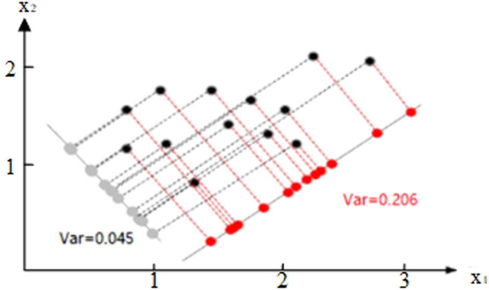
Schematic diagram of the projection variance of sample points.

2.2 Anomaly detection of T 2 statistic

Anomaly detection based on principal component analysis usually uses the T 2 statistic to detect whether the process is anomalous. The T 2 statistic measures the variation of variables in the principal component space. The detection function is as follows:

where x is the vector of correlation coefficients of the samples, Λ = diag { λ 1 , ⋯ , λ k } , and T α 2 is the T 2 control limit with confidence degree.

where F k , p − k ; α is the F distribution with the first degree of freedom k and second degree of freedom p − k .  α is usually taken as 0.01, 0.5, and 0.1. The test samples should satisfy T 2 ≤ T α 2 , otherwise it is judged as abnormal.

2.3 Further identification of anomalous telemetry

After the anomaly is detected by the earlier method, the data in the low-dimensional space are reconstructed into the high-dimensional space. The reconstruction error between the reconstructed high-dimensional data and the original low-dimensional data, as well as the contribution ratio of each component to the reconstruction error, is calculated. The larger the contribution ratio, the higher the possibility of an anomaly in that component. The telemetry parameters with anomalies can be roughly determined by cross-referencing the components with larger contribution ratios, which will serve as clues for further identification of fault locations.

The reconstruction error equation is as follows:

where X is the original high-dimensional data, and X ˆ is the reconstructed high-dimensional data. X ˆ is calculated as:

where A is the transformation matrix, and X ¯ is the mean value of the original high-dimensional data.

The proportion of each component to the reconstruction error is calculated as:

where X i j denotes the j th component of the i th original data, X ˆ i j the j th component of the i th reconstructed data, and U i denotes the reconstruction error of the i th original data.

3.1 Anomaly description

The following is an analysis of a power subsystem failure on one meteorological satellite. When the satellite entered the contact pass, the downloaded telemetry data indicated an anomalous telemetry voltage jump of one discharge module, from 28.79 to 54 V. Data playback showed that this voltage anomaly occurred at 5:46:24 the day before. After that, the telemetry voltage was maintained in an abnormal state. The telemetry curve directly reflecting the abnormal state is shown in Figure 2.

Figure 2

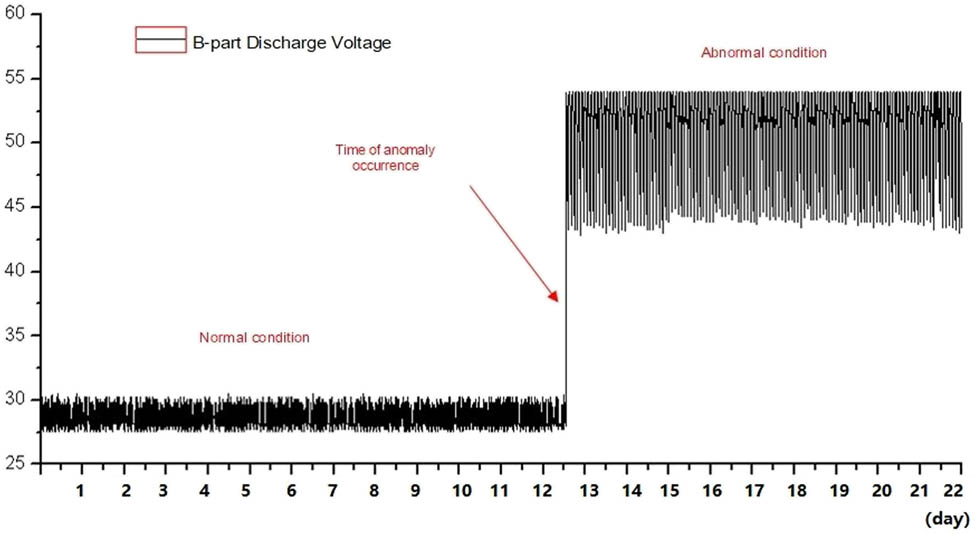
Telemetry curve directly correlated with the anomaly.

After the analysis of the data before and after the failure, the onboard power demand was just around the solar panel output power limit at the moment of the failure in the discharge regulator circuit, which resulted in frequent switch on/off of the discharge regulator controlled by the shunt error amplification signal and caused a high-power shock on the discharge regulator tube. Therefore, the most likely cause of the discharge regulator circuit failure is the short-circuit failure of the discharge regulator tube after the power shock. From Figure 2, it can be seen that the telemetry voltage of the B-channel discharge module (5) presented a sudden jump. In order to investigate the evolution of the satellite from normal to deviation and further to an anomaly, all features related to the anomaly need to be extracted. A total of 69 telemetry channels and 3,715,104 sample data were extracted from telemetry data collected within 1 month before and after the anomaly, respectively. In order to reduce the computational effort, 1/32 uniform sampling was performed on the samples, resulting in a total of 116,097 samples. Because some telemetry samples were correlated with the anomaly, and others were not, irrelevant telemetry needed to be eliminated.

3.2 Feature extraction

The telemetry was rejected according to the standard deviation. For telemetry that maintains a constant value throughout the process, the correlation with any telemetry or anomalies is zero. Initial statistics were performed for power subsystem telemetry. Since each telemetry represented a different physical meaning and range of values, the telemetry was first standardized to observe the fluctuation of each telemetry on the same scale. The standardized value of the telemetry fell in the range of [0,1]. The variance is then calculated for each telemetry, and we find that part of the telemetry signal is equal to 0 or close to 0. Combined with expert experience, it was determined that these telemetries were not related to anomalous states from a physical mechanism and were, therefore, excluded from the sample.

The satellite anomaly subsystem has at least dozens and even hundreds of telemetry. Each sample characterizes a point in a high-dimensional space, and the distribution of the samples in the high-dimensional space is unobservable. Therefore, the features need to be downscaled. On the other hand, in the subsequent anomaly identification, having too many features as the input to the algorithm will cause relatively large computation, and nonrelated telemetry input may also impact the algorithm’s convergence. It is necessary to reduce the dimensions of the anomaly features from the points of visualization, computational effort, and algorithm convergence.

In this article, to visualize the evolution of the satellite from normal to deviation to abnormality, the abnormal features were reduced in dimensionality by the principal component analysis method.

The dimension reduction will lead to the loss of information. The more the dimensions are reduced, the more information will be lost. After the dimension reduction of telemetry related to this anomaly for a satellite, the relationship between the information retention rate and the number of retained dimensions is shown in Figure 3.

Figure 3

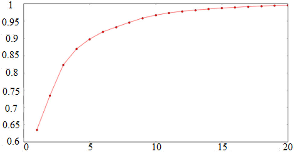
Information retention rate and retained dimensions.

Table 1 shows the information retention rate and the dimensions.

As shown in Figure 3, the information retention rate was about 63 % when the dimensions of power subsystem telemetry were reduced from 63 to 1 (5 telemetry had already been eliminated by the variance method). The retention rate was 73 % when the dimensions were reduced to 2. The rate was 99.6 % when the dimensions were reduced to 20, which implied that the 20 features contained 99.6 % of information in the original data, with an information loss of only 0.42.

4.1 Time-domain visualization

Satellite telemetry data are typical time-series data, whereas time-domain visualization is the most intuitive way to visualize the anomaly evolution. In the time-domain visualization, we drew the telemetry curves aligned with time, and investigated the evolution process by observing the telemetry curves, as shown in Figures 4, 5, 6.

Figure 4

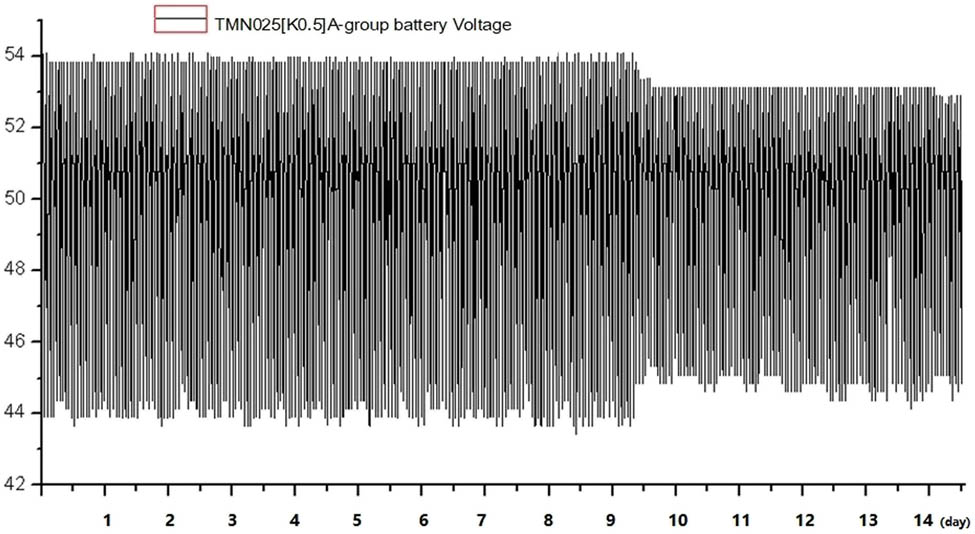
Battery voltage.

Figure 5

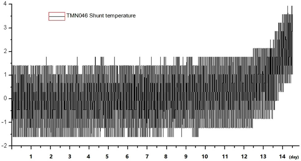
Shunt temperatures.

Figure 6

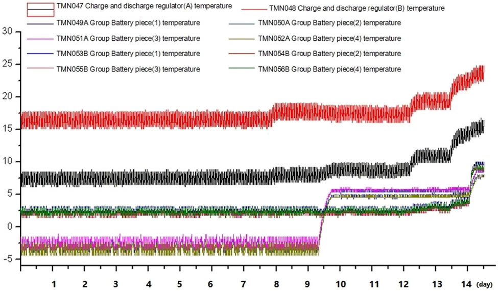
Battery pack temperatures.

4.2 Two-dimensional visualization

First, we downscaled all the extracted telemetry samples to two dimensions and displayed them on a two-dimensional diagram, as shown in Figure 7(a). The purple color in the figure denotes the normal sample points and the red denotes the abnormal sample points.

Figure 7

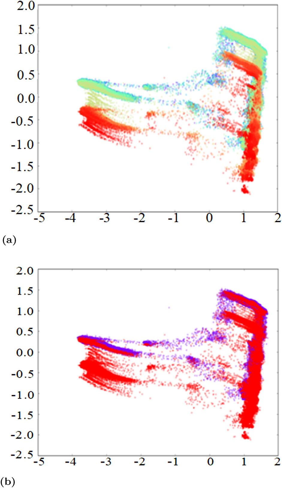
Two-dimensional diagram showing the anomaly evolution process. (a) Two-dimensional gamut map and (b) Two-dimensional gamut map of large sample.

The following conclusions can be drawn from the analysis of the earlier figure.

1. After the multidimensional features were reduced to two dimensions, there was a large portion of overlap between the two types of samples, which indicates that the classifier cannot distinguish well between normal and abnormal if two-dimensional features are used as input in the subsequent identification of the anomaly evolution process. Therefore, it is also necessary to expand the number of features to classify the two types of samples in a high-dimensional space.

2. Whether normal or abnormal samples, there was a large dispersion, which was due to the constantly changing power supply operating state during the satellite’s operation in orbit, including the battery charging/discharging state, the temperature of each battery, and the charging/discharging current.

3. The anomalous samples were more dispersed, and the center of gravity of the sample points had a significant shift before and after the anomaly occurred, indicating that there was a shift in the location of the sample distribution in the high-dimensional space.

As can be seen from the figure, with the passage of time, there was no obvious change in the position of the sample points when the sample was not abnormal, i.e., the green sample points in the figure. When the abnormality occurred, the position of the sample points gradually shifted, as shown in the earthy yellow sample points, and finally reached the position of the red sample points, i.e., the abnormal points.

4.3 3D visualization

We downscaled the telemetry of the power subsystem to a 3D, as shown in Figure 8(a), with the red color indicating the normal sample points and blue color indicating the abnormal samples. As can be seen from the figure, the differentiation of the two types of sample points in the three-dimensional space was improved relative to the two-dimensional, and the red samples had better aggregation. As the state changes to abnormal, the distribution of the samples in the three-dimensional space changes accordingly, as shown in the blue sample points, but some of the sample points and the red samples have overlapped.

Figure 8

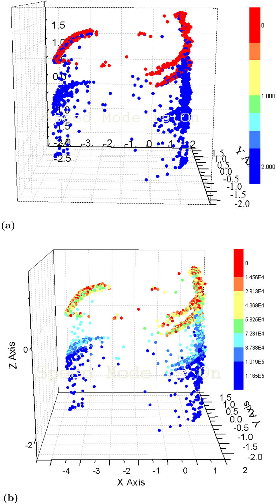
Three-dimensional diagram showing the anomalous evolution process. (a) 3D point cloud image and (b) 3D point cloud image of large sample.

In order to observe the evolution process of satellite status from normal to deviation to abnormal in more detail, the sample color was correlated with time, and the three-dimensional diagram was shown with the gradual change of time. As can be seen from Figure 8(a), the first 58,000 samples were more concentrated in distribution and were normal samples; the 58,000th to 87,000th samples gradually transitioned from normal to abnormal (the obvious abnormal point starts with the 62,000th sample); the 87,000th and later samples had been clearly separated from the normal samples, and, the subsequent classifier may be able to identify them effectively.

4.4 Visualization method analysis

The advantages and disadvantages of the three visualization methods can be summarized as: (i) Time-domain method is more intuitive with easy curve drawing. However, each diagram can only present one or a few telemetries. To fully understand all the information of anomaly, it is necessary to analyze all the telemetry one by one, which is unrealistic due to a large number of telemetries and a huge workload. (ii) Both two- and three-dimensional visualization can be classified as spatial visualization, where all changes in telemetry can be reflected in one diagram with a big picture. However, dimension reduction has to be performed, which will introduce information loss, resulting in incomplete and unintuitive information in the diagram.

References

Bolandi H, Abedi M, Haghparast M. 2013. Fault detection, isolation and accommodation for attitude control system of a three-axis satellite using interval linear parametric varying observers and fault tree analysis. J Aerosp Eng. 228(1):1403–1424. 10.1177/0954410013493230Search in Google Scholar
Bonfe M, Castaldi P, Geri W, Simani S. 2006. Fault detection and isolation for on-board sensors of a general aviation aircraft. Int J Adapt Control. 20(8):381–408. 10.1002/acs.906Search in Google Scholar
Flores-Abad A, Ma O, Pham K, Ulrich S. 2014. A review of space robotics technologies for on-orbit servicing. Prog Aerosp. 68(12):1–26. 10.1016/j.paerosci.2014.03.002Search in Google Scholar
Gao C, Duan G. 2014. Fault diagnosis and fault tolerant control for nonlinear satellite attitude control systems. Aerosp Sci Technol. 33(1):9–15. 10.1016/j.ast.2013.12.011Search in Google Scholar
Gueddi I, Nasri O, Benothman K, Dague P 2017. Fault Detection and Isolation of spacecraft thrusters using an extended principal component analysis to interval data. Int J Control Autom. 15(2):776–789. 10.1007/s12555-015-0258-xSearch in Google Scholar
Hou Y, Cheng Q, Qiu A, Jin Y. 2015. A new method of sensor fault diagnosis for under-measurement system based on space geometry approach. Int J Control Autom. 13(1):39–44. 10.1007/s12555-013-0514-xSearch in Google Scholar
Hu QL, Jiang CC. 2021. Relative Stereovision-based navigation for noncooperative spacecraft via feature extraction. IEEE/ASME Trans Mech. 10(11):1–11. 10.1109/TMECH.2021.3128402Search in Google Scholar
Ke L, Wu Y, Yi S. 2017. A novel method for spacecraft electrical fault detection based on FCM clustering and WPSVM classification with PCA feature extraction. J Aerosp Eng. 231(1):98–108. 10.1177/0954410016638874Search in Google Scholar
Li HN. 2010. Geostationary satellite orbital analysis and collocation strategies. BeiJing: National Defence Industry Press. Search in Google Scholar
Li WJ, Cheng XG, Wang YB. 2019. On-orbit service (OOS) of spacecraft: A review of engineering developments. Prog Aerosp. 108(5):32–40. 10.1016/j.paerosci.2019.01.004Search in Google Scholar
Marton L. 2015. Actuator fault diagnosis in mechanical systems-fault power estimation approach. Int J Control Autom. 13(1):110–119. 10.1007/s12555-013-0439-4Search in Google Scholar
Opromolla R, Fasano G, Rufino G, Grassi M. 2017. Pose estimation for spacecraft relative navigation using model-based algorithms. IEEE Trans Aerosp Electron. 53(1):431–437. 10.1109/TAES.2017.2650785Search in Google Scholar
Sun L, Huo W. 2016. Adaptive fuzzy control of spacecraft proximity operations using hierarchical fuzzy systems. IEEE/ASME Trans Mech. 21(3):1629–1640. 10.1109/TMECH.2015.2494607Search in Google Scholar
Tipaldi M, Bruenjes B. 2014. Spacecraft health monitoring and management. Proceedings of the 2014 IEEE Metrology for Aerospace. 2014 May 29-30; Benevento, Italy. IEEE, 2014. p. 68–72. Search in Google Scholar
Tong S, Huo B, Li Y. 2014. Observer-based adaptive decentralized fuzzy fault-tolerant control of nonlinear largescale systems with actuator failures. IEEE Trans Fuzzy Syst. 22(1):1–15. 10.1109/TFUZZ.2013.2241770Search in Google Scholar
Wu ZQ, Yang Y, Xu CH. 2015. Adaptive fault diagnosis and active tolerant control for wind energy conversion system. Int J Control Autom. 13(1):20–25. 10.1007/s12555-013-0148-zSearch in Google Scholar
© 2022 Na Fu et al., published by De Gruyter
This work is licensed under the Creative Commons Attribution 4.0 International License.
Articles in the same Issue
- Research Articles
- Deep learning application for stellar parameters determination: I-constraining the hyperparameters
- Explaining the cuspy dark matter halos by the Landau–Ginzburg theory
- The evolution of time-dependent Λ and G in multi-fluid Bianchi type-I cosmological models
- Observational data and orbits of the comets discovered at the Vilnius Observatory in 1980–2006 and the case of the comet 322P
- Special Issue: Modern Stellar Astronomy
- Determination of the degree of star concentration in globular clusters based on space observation data
- Can local inhomogeneity of the Universe explain the accelerating expansion?
- Processing and visualisation of a series of monochromatic images of regions of the Sun
- 11-year dynamics of coronal hole and sunspot areas
- Investigation of the mechanism of a solar flare by means of MHD simulations above the active region in real scale of time: The choice of parameters and the appearance of a flare situation
- Comparing results of real-scale time MHD modeling with observational data for first flare M 1.9 in AR 10365
- Modeling of large-scale disk perturbation eclipses of UX Ori stars with the puffed-up inner disks
- A numerical approach to model chemistry of complex organic molecules in a protoplanetary disk
- Small-scale sectorial perturbation modes against the background of a pulsating model of disk-like self-gravitating systems
- Hα emission from gaseous structures above galactic discs
- Parameterization of long-period eclipsing binaries
- Chemical composition and ages of four globular clusters in M31 from the analysis of their integrated-light spectra
- Dynamics of magnetic flux tubes in accretion disks of Herbig Ae/Be stars
- Checking the possibility of determining the relative orbits of stars rotating around the center body of the Galaxy
- Photometry and kinematics of extragalactic star-forming complexes
- New triple-mode high-amplitude Delta Scuti variables
- Bubbles and OB associations
- Peculiarities of radio emission from new pulsars at 111 MHz
- Influence of the magnetic field on the formation of protostellar disks
- The specifics of pulsar radio emission
- Wide binary stars with non-coeval components
- Special Issue: The Global Space Exploration Conference (GLEX) 2021
- ANALOG-1 ISS – The first part of an analogue mission to guide ESA’s robotic moon exploration efforts
- Lunar PNT system concept and simulation results
- Special Issue: New Progress in Astrodynamics Applications - Part I
- Message from the Guest Editor of the Special Issue on New Progress in Astrodynamics Applications
- Research on real-time reachability evaluation for reentry vehicles based on fuzzy learning
- Application of cloud computing key technology in aerospace TT&C
- Improvement of orbit prediction accuracy using extreme gradient boosting and principal component analysis
- End-of-discharge prediction for satellite lithium-ion battery based on evidential reasoning rule
- High-altitude satellites range scheduling for urgent request utilizing reinforcement learning
- Performance of dual one-way measurements and precise orbit determination for BDS via inter-satellite link
- Angular acceleration compensation guidance law for passive homing missiles
- Research progress on the effects of microgravity and space radiation on astronauts’ health and nursing measures
- A micro/nano joint satellite design of high maneuverability for space debris removal
- Optimization of satellite resource scheduling under regional target coverage conditions