Explaining the cuspy dark matter halos by the Landau–Ginzburg theory

1 Introduction

Cosmological simulations have revealed many almost universal properties of the “isolated” equilibrium cold dark matter halos (Navarro et al. 1997, 2010), and the most prominent one may be the NFW density profile, which shows the inner density slope − 1 and the outer slope − 3 . Recently, Wang et al. (2020) in their simulations shows that this universality can extend to the halos over twenty orders of magnitude in mass. Because the halos have finite mass, the outer slope should be smaller than − 3 , while outside the virial radius, there is a bump caused by the halos’ neighbor in the density profile (Francisco et al. 2006). Therefore, the outer slope should be shallower than some value, so it may be trivial that the outer slope is about − 3 , and most of the attentions have been paid to the inner slope. Because of its universality, any explanations invoking the initial conditions may be not convincing enough, therefore, although there are still other schemes (Dalal et al. 2010, Hansen and Sparre 2012, Dekel et al. 2003, Eilersen et al. 2017), the method of statistical mechanics is still always used trying to find the common physical origin of the cusps. For example, Hjorth and Williams (2010) assumed that the microstates should be counted in energy space and modifies the Stirling approximation in statistical mechanics, and they can show the r − 1 cusp; however, Destri (2018) found that Hjorth and Williams (2010)’s model can also allow the existence of the central core; Pontzen and Governato (2013) believed that, in the canonical ensemble, there exists another constraint caused by incomplete relaxation, but predicted much less low angular momentum orbits than simulations; Padmanabhan (2002) obtained the − 3 outer and − 1 inner slope of the dark matter halos by theoretical calculation, but he assumed that each halos have the same mass. Moreover, the new developments in studies of the vector resonant relaxation and isotropic-nematic phase transition (Kocsis and Tremaine 2015, Roupas et al. 2017, Roupas 2020) also indicate the great potential of statistical mechanics for self-gravitating systems. However, the statistical mechanics for self-gravitating systems still faces some challenges, such as the in-equivalence of ensembles, the broken of ergodicity, the thermodynamical limit problem, and so on (a recent review by Campa et al. 2014).

In this article, the almost universal r − 1 cusp will be explained by the LG theory, which is always used to study the system’s long-range correlations of fluctuations from the equilibrium state in the canonical ensemble (Plischike and Birgersen 2006), such as these studies of the density profile in the vapor–liquid interface, the LG coherence length in superconductivity, and others (Drrbeck et al. 2018, Paoluzzi et al. 2018). This theory is from the generalization of the Landau’s mean field theory (MFT) of phase transition near the critical point, and the physical meaning behind the MFT is clear, although it is not the most precise theory. Here, we do not prepare to study the phase transition of the dark matter, and with the help of the LG theory, we just try to discuss the density fluctuations from the equilibrium state and the correlation function of the density fluctuations at different places. On the basis of the following points, we think that the LG model in the critical phenomenon can be used to study the gravitating system: in the short-range systems, MFT is only correct for the cases with more than four dimensions because it neglected the long-range correlation near the critical point, and it is an approximation of the renormalization group theory, while some works (Cannas et al. 2000, Tsuda and Nishimori 2014) have proved that the MFT is exact for a wide range of long-range systems, and Kocsis and Tremaine (2015) even used the mean-field model to study the phase transition in the self-gravitating system; moreover, the LG model is used to study the long-range correlation of the system near the critical point, and the gravitating system always has the long-range correlation. It should be noted that the MFT is only exact for the short-range systems with more than four dimensions, which means that the main topic in this article may be finally resolved by the renomalization group.

The structure of the content is as follows: in Section 2, we will briefly review the result of the LG theory by considering the fluctuations of the Helmholtz and Gibbs free energy; in Section 3, we will apply this theory for simulated dark matter halos; finally, we will conclude this study in Section 4.

2 Landau–Ginzburg theory

In the statistical physics, each thermodynamical equilibrium state corresponds to one statistical distribution of the mechanical states, and the value of the thermodynamical quantity is the ensemble-average of all the mechanical states in this statistical distribution. Therefore, there always exists the fluctuations from this average value. The LG theory just describes the long-range correlation of fluctuations from the equilibrium state at least in an approximate fashion (Plischike and Birgersen 2006). For the homogeneous and isotropic systems, the two-point correlation function is expressed as follows:

where ρ ( r ) is the density at r , and ρ ¯ denotes its averaged value in the system.

In this article, we do not consider the effects of fluctuating temperature. With fixed temperature and volume, the Landau–Ginzburg theory assumes that the fluctuation of Helmholtz free energy can be expanded to the even powers of the density fluctuation:

If the density fluctuation is not large enough, a 4 and the following terms will be neglected. In Landau’s MFT of the critical phenomenon, the fluctuation of the order parameter is not considered, i.e., b = 0 ; a 2 should change the sign when the temperature crosses the critical temperature, which causes the second-order transition. b > 0 means that Δ F may be partly contributed by the fluctuation of ρ , which is just the character of the LG model. In this article, we aim to study the density profile of the fluctuations, which requires the equilibrium state to be stable at ρ − ρ ¯ = 0 , so a 2 > 0 and b > 0 . From the Appendix, we can know that

where

is the correlation length. The aforementioned results indicate that the two-point correlation function C ( r ) ∝ 1 / r for r ≪ ξ .

In fact, the LG theory can describe the more general cases if there exists other generalized forces and coordinates (Plischike and Birgersen 2006): the Gibbs free energy G can be expressed as follows:

where T is the temperature, h is the external perturbation, and M is the order parameter. M can be the magnetization in the Ising model for magnetic materials, the local density in liquid–vapor interface, the wave function in BCS theory for superconductivity, or the spins on the lattice of the crystal, etc. ( h , M ) is a pair of generalized force and coordinate, which can influence the Gibbs free energy. Therefore, the following ρ ( r ) will denote the general order parameter. For the inhomogeneous system, G is the functional of ρ ( r ) and M = ∫ ρ ( r ) d 3 r . Notice that LG theory can be valid even for discrete systems, as long as ρ ( r ) can vary significantly over large enough distances. By (5) and (2), we have

By calculating the minimum of the Gibbs free energy, we yield

where the last term is obtained by integration by parts and demanding δ ρ = 0 at the surface, and ϕ ( r ) = ρ ( r ) − ρ ¯ . Eq. (7) describes the change of order parameter ρ with r . If h is assumed to happen at r = 0 and be localized, i.e.,

where δ ( r ) is the Dirac function, and (7)’s analytical solution in the spherical coordinate is expressed as follows:

where the other solution e r / ξ / r has been abandoned. (9) is “coincidentally” proportional to (3), which has been explained in page 96 of Plischike and Birgersen (2006). It should be emphasized that this proportionality can set up only if (8) still holds, and the physics behind it is that if the perturbation h is localized, the fluctuations of the order parameter with different scales can be still statistically independent, then from the Appendix, the two-point correlation function (3) can still set up and will be proportional to the fluctuations of the order parameter. Besides, with many cases (but not all) of h ( r ) , the fluctuation of the order parameter will always show an inner r − 1 cusp.

3 Applications for cold dark matter halos

We first show the long-range nature of gravitating system indicated by the LG theory. Let us consider the self-gravitating gas contained in a box, whose virial theorem is (Padmanabhan 2002) (here, we do not consider the short-distance cutoff) expressed as follows:

where T is the total kinetic energy, U is the total potential energy, P is the pressure on the wall, and V is the total volume. If U ≪ T , then 2 T = 3 P V just can describe the ideal gas in a confined container; for the self-gravitating system, U cannot be neglected, especially if the system is steady, 2 T + U = 0 and P = 0 . Therefore, Eq. (10) can describe the gas with different potential energies. From Zhang (2005), a 2 in Eq. (2) can be written as follows:

where μ is the gas’s mole mass. In the short-range system near the critical point, ∂ P ∂ n ¯ = 0 , i.e., a 2 = 0 , and the system shows the long-range correlation. For the usual self-gravitating gas, we rewrite Eq. (10) as follows:

where t = T / M , u = U / M , and M is the total mass of the gas. Then,

The value of the pressure P (so a 2 ) of the self-gravitating system will be smaller than its value of the ideal gas because of the existence of the potential energy, so the correlation length of the self-gravitating system is longer than the short-range system. Especially for the steady self-gravitating system without the wall, 2 T + U = 0 , P = 0 will result in a 2 = 0 , ξ → ∞ . Therefore, the LG model also presents the long-range nature of the gravitating system.

Then, we try to use the LG theory to study the structure of dark matter halos in simulations. The order parameter in the LG theory always corresponds to certain symmetries, while the density distribution also can reflect the symmetries of the system, such as that the homogeneous and isotropic systems have translational and rotational invariant symmetries. Like works in the vapor–liquid interface, the order parameter will be the density in this work to explain the cusps of dark matter halos in simulations.

In the background cosmology, the cosmological principle states that the Universe is homogeneous and isotropic at large scale, and the whole Universe can be described as the ideal fluid; the matter is modeled as the ideal gas with nonrelativistic particles, and its pressure is (p. 109 in the study by Mo et al. 2010) expressed as follows:

The pressure of the matter is commonly regarded as zero if k B T ≪ m c 2 . In the CDM scenario, the structure formation is “bottom up,” and when perturbations with the smaller scale have entered the nonlinear regime so that sheets, filaments, and halos successively form, there exists a larger scale l c , which is just at the linear regime. Above the scale l c , the matter is highly homogeneous and can be assumed to be at thermal equilibrium from Eq. (14) (chapter 4 in the study by Mo et al. 2010). We can try to use the LG model to discuss the density fluctuations from this equilibrium state and the correlation between them because the most important in the matter-dominated Universe is that the gravities between matters gradually play more and more important roles, the correlation between density perturbations naturally exists in the system due to the long-range nature of gravity, and the LG theory is just the mean-field theory with considering the long-range correlations between fluctuations in the critical phenomenon. Besides, at the first step, we will neglect the contributions of baryons and compare our results with the dark matter-only simulations in the matter-dominated Universe, and the dark matter halos will be the densest fluctuations with nearly spherical shape. Therefore, we will try to use the LG theory to explain the almost universal density profile of dark matter halos shown in simulations (Navarro et al. 1997, 2010), and the mean density ρ ¯ in Section 2 can be the critical density ρ c in the matter-dominated Universe.

One problem is that someone may worry about whether the terms with high powers of ρ − ρ c can be neglected in Eq. (2). Our explanation is that, first, we have numerically checked that these terms will not have an import role in determining the inner cusp of the dark matter halos; besides, in this part, we only consider the early age of the halo formation, i.e., the average density fluctuation δ = ρ / ρ c − 1 is just a little larger than 1; at the same time because the structure formation is “bottom-up” in the CDM model, and the scale of the first structure may be small enough that h ( r ) can be localized (i.e., Eq. (8)), and the resulting profile is Eq. (9), and if Eq. (9) is simply approximated by ρ ( r ) = ρ c r c exp ( 1 − r / r c ) / r with ρ ( r c ) = ρ c , we can calculate that the average density perturbation inside the radius of r c is about 1.13, which is consistent with our assumption; finally, in the critical phenomenon, the fluctuations near the critical point even can be infinitely large, and the mean-field LG theory still shows the critical indices close to those from the renormalization group, which convinces us that it may be useful to consider the LG theory at the first step. Then we consider the larger structures and assume that the LG theory is still valid based on the aforementioned analysis, but we need to explore the form of h ( r ) . Commonly, the Universe is simulated in a box with fixed number of particles N and size L and with periodic boundary condition, which may be consistent with the condition of the canonical ensemble. The effect of the external perturbation h ( r ) is that it can change the gravities between particles, which will contribute the gravitational potential energy between particles and induce the change of the density fluctuations. The aforementioned process can change the Gibbs free energy. Therefore, the gravitational effect caused by the external perturbation will be the generalized force corresponding to the generalized coordinate density fluctuation. In the spherical coordinates, the expression of the potential energy is expressed as follows:

so we suggest that the perturbation h ( r ) for the self-gravitating system is

where M h is the equivalent mass scale of h ( r ) , and we can find that if M h is close to zero, h ( r ) can tend to be Eq. (8). For the dark matter-only simulations with boxsize L , M h can be about 4 π ρ b ¯ L 3 / 3 , where ρ b ¯ is the average density of the matter in the box. In cosmology different scales of dark matter, halos can be virialized if M v i r = 200 ∗ 4 π ρ c r 200 3 / 3 , where ρ c is the critical density of the Universe and r 200 is the radius within which the spherically averaged density is 200 times the critical density. Then we can directly combine Eq. (16) with Eq. (7), and the analytical solution is

where c and ξ can be determined by ρ ( r 200 ) = ρ c and 4 π ∫ 0 r 200 ρ r 2 d r = M v i r . For the static collisionless system, there exists a similar equation with (10) (page 235 of Mo et al. 2010), but the term at the righthand side is the work done by the external pressure W = ∫ ρ σ 2 ¯ r d S ( σ is the velocity dispersion), which for the spherical static collisionless system is equal to 3 P b V , where P b = W / 3 V is the pressure at the boundary of the halo. Therefore, we can also use Eq. (13) to evaluate a 2 but with P = P b . Eq. (17) shows that the inner cusp is still r − 1 . If M h is small enough ( GM h ≪ a 2 c ), h ( r ) will reduce to (8), and (17) will return to (9). In Figure 1, we compare Eq. (17) and NFW.

Figure 1

The density profile of (17) compared with NFW. Eq. (17) satisfies the conditions with the central density ρ LG ( 0 ) = ρ NFW ( 0 ) , the total mass M LG = M NFW , and the radius R LG = R NFW = 9 r s where r s is the scale radius in the NFW profile.

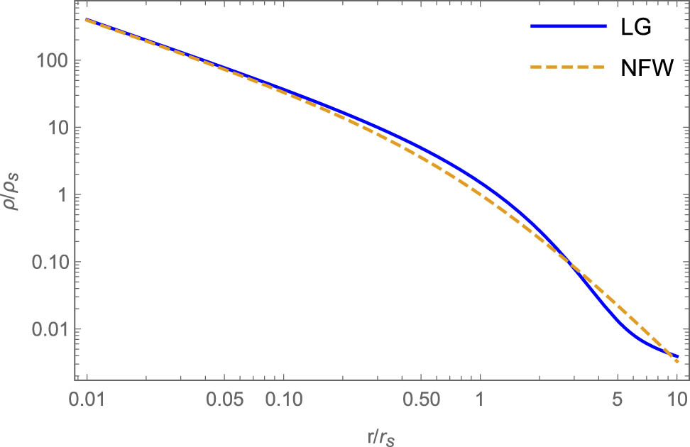
Eq. (9) is also close to the recent result of the study by Fielder et al. (2020) finding that the density profile of dark matter halos is better described by the generalized Einasto profile:

where γ and α are two parameters.

In the CDM scenario, the structure formation is bottom-up, and the larger halos is mainly from its progenitors’ mergers and accretions, and current simulations and theoretical analysis (El-Zant 2008, Syer and White 1998, Wang and White 2009) show that mergers and accretions will not change the inner r − 1 cusp. This work also supports this point, and we show that r − 1 cusp can form at the early stage of structure formation at each scale, which is consistent with the conclusion of Wang et al. (2020) that the cusps of halos with mass spanning more than 20 orders of magnitude are always r − 1 .

Besides, in the CDM scenario at time t , there exists a perturbation scale l h where the corresponding halos are just forming. At the scales smaller than l h the correlation function C ( r ) will scale as the density peak, so from Section 2 it is also proportional to r − 1 at the small scale. From the appendix we know that the LG theory shows the k − 2 power spectrum at the small scale. Both behaviors of C ( r ) and P ( k ) are also consistent with the analysis of Padmanabhan (2002), which shows that C ( r ) ∝ 1 / r for small r and n = − 2 (if the pow spectrum P ( k ) ∝ k n ) is the critical index in the nonlinear regime. For the scales larger than l h , it is not suitable to directly discuss them because there are other nonspherical structures such as sheets and filaments in the Universe. We will continue to study this issue in the future.

4 Discussion and conclusion

The LG theory is used to describe the fluctuations from the equilibrium state and to study the long-range correlations of fluctuations near the critical point in an approximate fashion, and the modern method is the renormalization theory of Wilson. This article first introduced this method, and then studied the fluctuations from the background equilibrium state of the homogenous and isotropic Universe in the CDM scenario. The gravitational instability and density perturbation can contribute to the Gibbs free energy, they are modeled as one pair of the generalized force and coordinate, and we make some approximations for the form of the gravitation instability. For the density fluctuations with the smallest scale, h ( r ) can be the Delta function, and with the assumptions of quasi-linear regime and the validity of the LG model, the inner r − 1 cusp can be obtained; for the larger scale, we suggest h ( r ) = GM h / r and the conclusion does not change. This may be consistent with the fact that the dynamical processes such as mergers and accretions do not change the inner cusp, and current works are also expected to show the existence of the inner r − 1 cusps for all the dark matter halos.

Our work indicates that the inner r − 1 cusp of the dark matter halos may originate from the long-range correlations of the fluctuations of the gravitating system. This correlation is common with other short-range or long-range systems near the critical point, such as that current ferromagnetic experiments and scattering experiments (Binney et al. 1992) also show that the two-point correlation function in the critical phenomena of three-dimensional systems is proportional to 1 / r 1 + η for large r compared with intermolecular distances, and η ∼ 0.07 is one of the critical indices, which also can be obtained from the theory of renormalization group. The difference is that, for the trivial short-range systems, the correlation length is very short on the macro level (except at the critical point), and the density fluctuations are not easily recognized; however, the correlation length in the gravitating system is much longer, and the smallest scale structures in the homogeneous and isotropic Universe still can be easily observed.

Padmanabhan (2002) also studied the physics behind the almost universal NFW profile. He assumed that the density field can be expressed as a superposition of several halos with the same mass, core radius etc and the correlation function is power law. Compared with his work, this article does not need to consider these assumptions, and we still obtained the critical k − 2 power spectrum in the nonlinear regime, which also appeared in Padmanabhan (2002). Here, we provide another train of thought to explain the universal r − 1 problem, but which may be still an open question. In the future work, we will continue to examine this idea and explore the possibility of completely solving it by the renomalization group. We also need to consider the issue of the cusp-core transformation.

References

Binney JJ, Newman MEJ, Fisher AJ, Dowrick NJ. 1992. The Theory of Critical Phenomena: An Introduction to the Renormalization Group. Oxford: Oxford University Press, Inc. 10.1093/oso/9780198513940.001.0001Search in Google Scholar
Campa A, Dauxois T, Fanelli D, Ruffo S. 2014. Physics of Long-range Interacting Systems. Bristol: IOP Publishing. 10.1093/acprof:oso/9780199581931.001.0001Search in Google Scholar
Cannas SA, de Magalhaes ACN, Tamarit FA. 2000. Evidence of exactness of the mean-field theory in the nonextensive regime of long-range classical spin models. PRB. 61:11521. 10.1103/PhysRevB.61.11521Search in Google Scholar
Dalal N, Lithwick Y, Kuhlen M. 2010. The Origin of Dark Matter Halo Profiles. arXiv:1010.2539. Search in Google Scholar
Dekel A, Arad I, Devor J, Birnboim Y. 2003. Dark halo cusp: asymptotic convergence. ApJ. 588:680.10.1086/374328Search in Google Scholar
Destri C. 2018. Cored density profiles in the DARKexp model. JCAP. 5:010. 10.1088/1475-7516/2018/05/010Search in Google Scholar
Drrbeck S, Hollerer M, Thurner CW, Redinger J, Sterrer M, Bertel E. 2018. Correlation length and dimensional crossover in a quasi-one-dimensional surface system. PRB. 98:35436. 10.1103/PhysRevB.98.035436Search in Google Scholar
Eilersen A, Hansen SH, Zhang XY. 2017. Analytical derivation of the radial distribution function in spherical dark matter haloes. MNRAS. 467(2):2061–2065.10.1093/mnras/stx226Search in Google Scholar
El-Zant AA. 2008. The persistence of universal halo profiles. ApJ. 681:1058. 10.1086/587022Search in Google Scholar
Fielder CE, Mao Y-Y, Zentner AR, Newman JA, Wu H-Y, Wechsler R. 2020. Illuminating dark matter halo density profiles without subhaloes. MNRAS. 499(2):2426–2444. 10.1093/mnras/staa2851Search in Google Scholar
Francisco P, Klypin AA, Simonneau E, Betancort-Rijo J, Patiri S, Gottlöber S, et al. 2006. How far do they go? The outer structure of galactic dark matter halos. ApJ. 645:1001. 10.1086/504456Search in Google Scholar
Hansen SH, Sparre M. 2012. A derivation of (half) the dark matter distribution function. ApJ. 756:100. 10.1088/0004-637X/756/1/100Search in Google Scholar
Hjorth J, Williams LLR. 2010. Statistical mechanics of collisionless orbits. I. Origin of central cusps in dark-matter halos. ApJ. 722:851. 10.1088/0004-637X/722/1/851Search in Google Scholar
Kocsis B, Tremaine S. 2015. A numerical study of vector resonant relaxation. MNRAS. 448(4):3265–3296. 10.1093/mnras/stv057Search in Google Scholar
Mo HJ, van den Bosch F, White SDM. 2010. Galaxy Formation and Evolution. New York: Cambridge University Press. 10.1017/CBO9780511807244Search in Google Scholar
Navarro JF, Frenk CS, White SDM. 1997. A universal density profile from hierarchical clustering. ApJ. 490:493–508. 10.1086/304888Search in Google Scholar
Navarro JF, Ludlow A, Springel V, Wang J, Vogelsberger M, White SDM, et al. 2010. The diversity and similarity of simulated cold dark matter haloes. MNRAS. 402(1):21–34. 10.1111/j.1365-2966.2009.15878.xSearch in Google Scholar
Padmanabhan T. 2002. Statistical mechanics of gravitating systems in static and cosmological backgrounds. In: Dauxois T, Ruffo S, Arimondo E, Wilkens M, Editors. Dynamics and Thermodynamics of Systems with Long-Range Interactions. Lecture Notes in Physics, Vol. 602. Berlin, Heidelberg: Springer. 10.1007/3-540-45835-2_7. Search in Google Scholar
Paoluzzi M, Marconi U, Maggi C. 2018. Effective equilibrium picture in the xy model with exponentially correlated noise. PRE. 97:022605. 10.1103/PhysRevE.97.022605Search in Google Scholar PubMed
Plischike M, Birgersen B. 2006. Equilibrium Statistical Mechanics. 3rd ed. Singapore: World Scientific Publishing Company. 10.1142/5660Search in Google Scholar
Pontzen A, Governato F. 2013. Conserved actions, maximum entropy and dark matter haloes. MNRAS. 430(1):121–133. 10.1093/mnras/sts529Search in Google Scholar
Roupas Z. 2020. Statistical mechanics of gravitational systems with regular orbits: rigid body model of vector resonant relaxation. JPA. 53:045002. 10.1088/1751-8121/ab5f7bSearch in Google Scholar
Roupas Z, Kocsis B, Tremaine S. 2017. Isotropic–Nematic Phase Transitions in Gravitational Systems. ApJ. 842:90. 10.3847/1538-4357/aa7141Search in Google Scholar
Syer D, White SDM. 1998. Dark halo mergers and the formation of a universal profile. MNRAS. 293(4):337–342. 10.1046/j.1365-8711.1998.01285.xSearch in Google Scholar
Tsuda J, Nishimori H. 2014. Mean-field theory is exact for the random-field model with long-range interactions. JPSJ. 83:074002. 10.7566/JPSJ.83.074002Search in Google Scholar
Wang J, White SDM. 2009. Are mergers responsible for universal halo properties? MNRAS. 396(2):709–717. 10.1111/j.1365-2966.2009.14755.xSearch in Google Scholar
Wang J, Bose S, Frenk CS, Gao L, Jenkins A, Springel V, et al. 2020. Universal structure of dark matter haloes over a mass range of 20 orders of magnitude. Nature. 585:39–42. 10.1038/s41586-020-2642-9Search in Google Scholar PubMed
Zhang Q-R. 2005. Statistical Mechanics (in Chinese), 2nd ed. Beijing: China Science Publishing. Search in Google Scholar
© 2022 Dong-Biao Kang and Tong-Jie Zhang, published by De Gruyter
This work is licensed under the Creative Commons Attribution 4.0 International License.
Articles in the same Issue
- Research Articles
- Deep learning application for stellar parameters determination: I-constraining the hyperparameters