Cooperative capture trajectory optimization of multi-space robots using an improved multi-objective fruit fly algorithm

Yong Wang; Jing Cao; Nan Ye; Shouming Sun; Junfeng Li; Zhenyong Bo

doi:10.1515/astro-2022-0198

Article Open Access

Cooperative capture trajectory optimization of multi-space robots using an improved multi-objective fruit fly algorithm

Yong Wang , Jing Cao , Nan Ye , Shouming Sun , Junfeng Li and Zhenyong Bo

Published/Copyright: December 21, 2022

Published by

Become an author with De Gruyter Brill

Submit Manuscript Author Information Explore this Subject

From the journal Open Astronomy Volume 31 Issue 1

Abstract

Considering that some tasks will require the consistency of the position and attitude of the end-effector, multi-space-robot cooperative capture also needs to consider the synchronization of the two capture arms. Taking the dual-space robots as example, the trajectory planning problem before cooperative capture is focused. First, a drive-transform method based on trapezoidal velocity interpolation is proposed, which combines the advantages of these two methods to obtain the SE(3) motion trajectory, in which the attitude and position are planned synchronously. Then, the trajectory optimization model of cooperative capture is established, which takes the optimal time and the minimum attitude disturbance of the base as the optimization goals, and simultaneously satisfies that the two capture arms reach the capture point synchronously. In order to solve this multi-objective optimization problem, a dual-population multi-objective fruit fly algorithm based on non-dominated sorting was proposed. Finally, the simulation example of dual-space robots shows that the proposed algorithm is effective, and the analysis of the optimal solution set demonstrates that the optimized cooperative capture trajectory is smooth and synchronous.

Keywords: space robots; cooperative capture; fruit fly algorithm; trajectory planning

1 Introduction

Space robot technology has always been one of the important options in on-orbit servicing technology (Yoshida 2007). On-orbit servicing can be applied to on-orbit refueling, on-orbit maintenance, module replacement, garbage cleaning, etc., (Chen et al. 2009, Liang et al. 2012). As one of the key technologies of on-orbit servicing, space manipulators can perform some important operations such as capture, detumbling, and transport (2007 and 2008). With the continuous expansion of service objects and the extremely high reliability requirements of space missions, (Friend 2008) single-arm and multi-arm space robots will face some incompetent operational tasks. The application of small satellites and the maturity of formation technology make it possible for multi-space robots to provide collaborative on-orbit servicing (Flores-Abad et al. 2014).

Rekleitis and Papadopoulos (2010, 2011, 2015) proposed the concept of using multiple free-flying service robots to cooperatively operate passive targets. Each robot is equipped with a manipulator arm and a switch thruster. By coordinating and controlling the direction of the external force applied by the manipulator arm, operations such as transport of passive targets can be realized. And the differences between multiple free-flying service robots and a single large space robot were also analyzed in detail (Rekleitis and Papadopoulos 2013). Boning and Dubowsky (2012) proposed the application of a team of automated space robots to build large-scale structures such as solar power stations and space telemetry stations in orbit. Each robot has different functions, including a multi-arm integrated robot, a transport robot, and an observation robot. Domestic scholars studied dual robots operating flexible beams in orbit (Yuan 2015). Other scholars studied formation flying space robots used for cooperative location (Zhai et al. 2014), non-cooperative targets operation (Zhai et al. 2013, Gao 2015), and mission planning (Wu et al. 2014).

Trajectory planning is very important for robotics (Lei 2020). The abstract operation task is transformed into exact trajectory by the planner, which is used as the input of the control mechanism (Chen 2021). Trajectory planning usually includes planning in joint space and in Cartesian space, which refer to the planning of joint variables and planning of trajectory of the end-effector, respectively. Both of them are very important, but usually selected according to the application requirements (Chujo et al. 2020). The planning in joint space can generate continuous smooth and non-singular joint trajectory. The disadvantage is that the trajectory of the end-effector in Cartesian space is not intuitive. Moreover, the trajectory planning in Cartesian space is suitable for some special tasks with strict constraints on the trajectory of the end-effector. For example, when the end effector pulls out a device during on-orbit maintenance, it is required that the end effector must move in a straight line to avoid unnecessary contact or collision (Chujo et al. 2020). According to the task requirements (Wang 2020), trajectory planning in Cartesian space includes point-to-point planning and continuous path planning. The continuous path can be interpolated to obtain multiple intermediate nodes if necessary.

Compared with traditional single-arm and multi-arm space robots, the cooperative capture by multi-space robots has many advantages and development potentials, such as:

The coordination of multiple robots can disperse the valuable payloads, and separate tasks, which can avoid the failure of the whole mission caused by problems of a certain robot or arm.
During on-orbit operation, capture and fixation of the target is one of the key steps. Cooperative capture of huge target can effectively improve the stability of the system and flexibility of the task.
The cost of on orbit operation tasks is very high, and small mass satellites have the characteristics of low launch cost, strong mobility and fuel saving. Taking advantage of these advantages, developing multi-space robots with small mass satellites as the carrier, and then flexibly combining them, can greatly improve the diversity and reusability of tasks.

For multi-space robots service system, the cooperative motion of each space robot must be considered during the trajectory planning in Cartesian space. The two capture arms need to reach the capture point at the same time during a capture process. On the one hand, it can reduce capture time and improve efficiency, which is very critical for some tasks with operating time restrictions; on the other hand, it can also ensure that the two arms can capture and fix the target at the same time, and then perform a stable operation to the target. It can avoid the interruption between systems and ensure the mission successfully. In addition, the execution of a single task usually needs to optimize multiple goals to meet different requirements such as the efficiency, reliability, and fuel. The goals usually include working time, base disturbance, and joint energy consumption. This work takes the dual-space robots as example to study the multi-objective collaborative planning problem for the point-to-point terminal of the two arms.

2 Cooperative capture system model

The cooperative capture system consists of a dual-arm space robot and a single-arm space robot (for convenience, hereinafter referred to as dual-arm system and single-arm system, respectively). Figure 1 presents a simplified model of the pre-capture system. The definitions of the symbols in the figure are as follows:

Σ_G represents the global inertial reference frame. Generally, the origin of the coordinate system can be placed at the center of mass of the capture system;
Σ_DI, Σ_SI, and Σ_T represent the fixed coordinate systems of the dual-arm system, the single-arm system, and the capture target, respectively, whose origins are located at their center of mass;
Vector ^G p _d represents the position vector of the center of mass of the dual-arm system in the global inertial frame;
Vector ^G p _s represents the position vector of the center of mass of the single-arm system in the global inertial frame;
Vector ^G p _t represents the position vector of the target center of mass in the global inertial frame.

Figure 1

A simplified model of the cooperative capture system.

3 Drive-transform method based on trapezoidal velocity interpolation

3.1 Linear path planning based on drive-transform method

The core idea of the drive-transform method is to use the constructed drive transform function to express the configuration of the end-effector. Moreover, in order to maintain the consistency of position and attitude, the configuration of the end-effector is expressed in a homogeneous form during the planning process. In fact, based on its own advantages of unity, it will be more convenient to apply theories of Lie groups and Lie algebras for derivation and planning. Here the derivation process of the drive-transform method is given by applying the Lie group SE(3) and the screw theory.

First, divide the motion process of the end-effector into N segments, with a total of N + 1 nodes. Assuming that the configuration of the end-effector at each node is known, which is expressed as g _i ∈ SE(3) (i = 0, 1,…, N). t _i represents the time corresponding to the i th node, as shown in Figure 2. The motion of the end-effector between t _i and t _i+1 is discussed below.

Figure 2

A sketch map of drive-transform method.

The configuration of the end-effector at time t is expressed by the following function,

(1) g ( t ) = g i D ( h ) ,

where D(h) is the drive-transform function. h is the normalized time expressed as

(2) h = t − t i t i + 1 − t i .

Obviously, 0 ≤ h ≤ 1.

According to the boundary constraints, the following conditions must be met,

(3) g ( 0 ) = g i D ( 0 ) = g i , g ( 1 ) = g i D ( 1 ) = g i + 1 ,

then there is,

(4) D ( 0 ) = E 4 × 4 , D ( 1 ) = g i − 1 g i + 1 .

Linear planning from g _i to g _i+1 can be achieved using the drive-transform function. And D(1) can be explained as the deviation of the configuration between t _i and t _i+1.

It is easy to know from the characteristic of SE(3) that D(h) ∈ SE(3). Then, let

(5) g i = R i p i 0 1 , g i + 1 = R i + 1 p i + 1 0 1 ,

as well as

(6) D ( h ) = R D ( h ) p D ( h ) 0 1 .

Substituting this equation in Eq. (4), then,

(7) D ( 0 ) = R D ( 0 ) D 0 1 = E 3 × 3 0 0 1 ,

(8) D ( 1 ) = R D ( 1 ) p D ( 1 ) 0 1 = g i − 1 g i + 1 = R i T R i + 1 R i T ( p i + 1 − p i ) 0 1 .

Performing linear planning of the translational part first, assume

(9) p D ( h ) = h c 1 + c 0 ,

where c ₁ and c ₀ are constant vectors. According to formulas (7) and (8), it can be obtained that

(10) c 1 = p D ( 1 ) = R i T ( p i + 1 − p i ) , c 0 = 0 .

Then, do a linear planning of the rotating part. As is known, R _D(0) = E _3×3, and R _D(1) can be expressed in exponential form as

(11) R D ( 1 ) = R i T R i + 1 = e θ e ω ˆ e ,

where θ _w and ω ˆ e can be obtained by the axis-angle method.

Let,

(12) R D ( h ) = e h θ e ω ˆ e ,

R _D(0) and R _D(1) can be satisfied. So, the expression for D(h) is,

(13) D ( h ) = e h θ e ω ˆ e h R i T ( p i + 1 − p i ) 0 1 .

Finally, the trajectory of the end-effector can be planned as,

(14) g ( h ) = g i D ( h ) = R i p i 0 1 e h θ e ω ˆ e h R i T ( p i + 1 − p i ) 0 1 = R i e h θ e ω ˆ e h p i + 1 + ( 1 − h ) p i 0 1 .

3.2 Improved drive-transform method

The motion velocity between two nodes planned by the drive-transform method is a constant value. Considering that there must be a start and stop process when the joint is driven, the acceleration and deceleration process of the trajectory must be considered during motion planning. At the same time, the selection of nodes also needs to be prudent, too many nodes will inevitably increase the amount of calculation, and too few nodes may decrease the accuracy of the trajectory.

Trapezoidal velocity interpolation can describe the motion process well and satisfies continuity. However, the trapezoidal velocity interpolation is only suitable for the planning of the translational part, while the attitude planning has to be done separately, which leads to inconvenience. The drive-transform method can just make up for this. Therefore, we propose an improved drive-transform method based on trapezoidal velocity interpolation to carry out the planning of the configuration of the end-effector in Cartesian space.

According to the definition of variables in Section 3.1, the initial moment and the configuration of the end-effector are given, respectively.

(15) g 0 = R 0 p 0 0 1 , g n = R n p n 0 1 .

Deviation of the configuration is

(16) g f = g 0 − 1 g n = R 0 T R n R 0 T ( p n − p 0 ) 0 1 .

First, linear velocity of the end-effector is planned. Let the distance to the initial position at time t be d(t), and d(0) = 0, so

(17) d ( t f ) = d f = ‖ p n − p 0 ‖ .

In order to meet the smoothness requirements at the same time, the trapezoidal velocity interpolation with parabolic transition is used, as shown in Figure 3, where v(t) denotes the linear velocity of the end-effector, v _c denotes the linear velocity of the constant velocity stage, which is the maximum linear velocity, and t _s denotes the end time of the constant velocity. From this, the equation of the linear trajectory can be given as follows

(18) d ( t ) = 3 v c 4 t a 2 t 3 , if 0 ≤ t < t a 3 , d ( t ) = v c 4 t − t a 3 + 3 v c 4 t a t − t a 3 2 + v c t a 36 , if t a 3 ≤ t < 2 t a 3 , d ( t ) = v c t − 2 t a 3 − 3 v c 4 t a 2 ( t − t a ) 3 + v c t a 6 , if 2 t a 3 ≤ t < t a , d ( t ) = v c ( t − t a ) + v c t a 2 , if t a ≤ t < t s , d ( t ) = v c ( t − t s ) − 3 v c 4 t a 2 ( t − t s ) 3 + v c t s − v c t a 2 , if t s ≤ t < t s + t a 3 , d ( t ) = 3 v c t 4 − 3 v c 4 t a t − t s − t a 3 2 + v c t s 4 − 4 v c t a 9 , if t s + t a 3 ≤ t < t s + 2 t a 3 , d ( t ) = 3 v c 4 t a 2 ( t − t a − t s ) 3 + v c t s , if t s + 2 t a 3 ≤ t ≤ t s + t a .

Figure 3

Diagram of trapezoidal velocity interpolation with parabolic transition.

Then, the total movement time is jointly determined by

(19) t f = t s + t a = d f / v c + t a .

The above planning can only satisfy the requirement that the motion path of the end-effector is a straight line, but cannot express complete configuration, that is, the variation of attitude is missing. At the same time, the joint variables cannot be solved only from the above planning results. Therefore, it is necessary to use the above results as the initial conditions of the drive-transform function. So, the entire movement process is divided into seven stages, with a total of eight nodes, and the corresponding moments of each node are as follows:

(20) t i = i t a 3 , i = 0 , 1 , 2 , 3 , t i = t s + ( i − 4 ) t a 3 , i = 4 , 5 , 6 , 7 .

The configuration of each node is

(21) g i = R i p i 0 1 = g 0 g i e = g 0 R i e p i e 0 1 ,

where the translational part of g _ie is

(22) p i e = d ( t i ) d f R 0 T ( p n − p 0 ) .

The rotating part is,

(23) R i e = e d ( t i ) d f θ f ω ˆ f ,

where θ _f and ω ˆ f can be solved by the axis-angle method according to

(24) R 0 T R n = e h θ f ω ˆ f .

In addition, there is a very important step: normalize the time between nodes, which is given by the following formula

(25) h ( t ) = d ( t ) − d ( t i ) d ( t i + 1 ) − d ( t i ) , t i ≤ t < t i + 1 .

Substitute Eqs. (20)–(25) in Eq. (14) to obtain the continuous trajectory equation of the end-effector. Only v _c and t _a are variable in the planning process. And there is

(26) t a = 3 v c 2 a c ,

where a _c is the maximum angular velocity. v _c and a _c can be used as the decision variables while optimizing.

4 Multi-objective cooperative planning problem for multi-space robots

4.1 Description of cooperative planning problem

Section 3.2 presents a point-to-point linear path planning method for a single-space robot. For the multi-space-robot service system, the coordination of the two capture arms must be considered. In order to distinguish the two systems, subscripts ()_s and ()_d are added to the right of the above quantities.

When a set of decision variables v _cs, a _cs, v _cd, and a _cd of the dual-robot system is given, the total movement time of each can be calculated separately

(27) t f s = d f s v c s + 3 v c s 2 a c s , t f d = d f d v c d + 3 v c d 2 a c d .

The capture mechanisms at the end of the arms are, respectively, close to the capture point. In order to stabilize as soon as possible after capture, it is desired that the arms reach the target as simultaneous as possible.

(28) | t f s − t f d | < ε t ,

where ε _t is a small amount, which can be set according to the task accuracy requirements.

In addition, in order to make sure the cooperative approaching process is safe and reliable, it is necessary to ensure that the movement process of the two arms is basically synchronized, so the following constraint is given:

(29) ∑ i = 0 7 d ( t i s ) d f s − d ( t i d ) d f d < ε d ,

where ε _d is the threshold value.

In addition to the constraints generated by the coordinated motion, the joint limit will also determine the range of the decision variables v _cs, a _cs, v _cd, and a _cd

(30) v c s min ≤ v c s ≤ v c s max , a c s min ≤ a c s ≤ a c s max , v c d min ≤ v c d ≤ v c d max , a c d min ≤ a c d ≤ a c d max .

4.2 Analysis of optimization goals

In order to improve the execution efficiency of the task, the total time of the end movement is required to be as short as possible. Considering constraints in Eq. (28), t _fd is chosen as optimization object, that is

(31) m i n : f 1 = t f d = d f d v c d + 3 v c d 2 a c d .

When the trajectory equations of the two capture arms are obtained by planning, the spatial velocities of the ends are, respectively,

(32) V d S E G = ( g ̇ d g d − 1 ) ∨ ,

(33) V s S E G = ( g ̇ s g s − 1 ) ∨ .

According to the definition of the generalized Jacobian matrix, the spatial velocities of the base of the dual-arm system and the single-arm system are, respectively,

(34) V d S B G = J B d J E d + V d S E G ,

(35) V s S B G = J B s J E s + V s S E G .

where J _Bd, J _Bs, J E d + , J E s + are the generalized Jacobian matrices of the base and end of the dual-arm system and the single-arm system, respectively.

Furthermore, the spatial angular velocity of the two bases ω d S ω s S can be obtained, respectively, then let

(36) v max d = max 0 ≤ t ≤ t f d { ( ω d S ) T ω d S } ,

(37) v max s = max 0 ≤ t ≤ t f s { ( ω s S ) T ω s S } .

At the same time, in order to avoid the instability of the base caused by the dynamic coupling, and considering the constraints of the communication orientation and the angle of the solar sail, it is required to minimize the disturbance to the attitude of the base during the motion process. Another optimization objective is designed as

(38) m i n : f 2 = v max d + v max s .

5 Strategy for the multi-objective optimization problem

5.1 The principle of Lèvy flight

Lèvy flight is a mathematical model that describes insect foraging flight strategies, that is, a combination of normal short-range random flight and occasional long-range flight. Its mathematical distribution is called the Lèvy distribution. The introduction of Lèvy flight into the evolutionary intelligent optimization algorithm can realize the effective combination of local and global search, and improve the global optimization ability of the algorithm.

Generally, the following formula is used to calculate the Lèvy flight distance:

(39) L s = α / | β | 1 / λ ,

where α obeys the normal distribution N ( 0 , σ α 2 ) , β obeys the normal distribution N(0,1), and λ is the adjustment parameter, usually 1.5. σ α 2 is given by

(40) σ α 2 = Γ ( 1 + λ ) × sin π λ 2 Γ 1 + λ 2 × λ × 2 λ − 1 2 1 λ .

5.2 Solution strategy based on multi-objective fruit fly algorithm

At present, the application of fruit fly algorithm to multi-objective optimization problems is still in the exploratory stage. In order to solve the proposed multi-objective planning problem and improve the optimization ability of the algorithm at the same time, the original fruit fly algorithm is improved, and a dual-population multi-objective fruit fly optimization algorithm is proposed. The solution flow based on this algorithm is as follows.

Step 1: Set constraints and calculation parameters, including population number N _p, search times N _s, search step S, boundary conditions P _min = [v _csmin a _csmin v _cdmin a _cdmin]^T, P _max = [v _csmax a _csmax v _cdmax a _cdmax]^T;

It should be noted that there are 4 variables in our problem, so the individual is actually a vector.

Step 2: Initialize the population position [X _pop, Y _pop]. Since the relationship between the decision variables and the fly position is not linear, it is difficult to directly convert the boundary conditions of the decision variables into constraints of the fly position. Therefore, the following initialization method is designed to obtain the initial population position that satisfies the constraints.

Two random numbers R rad ∈ ( 1 , inf ) , A rad ∈ 0 , π 4 are generated first, then, let

(41) X pop = R rad × cos ( A rad ) , Y pop = R rad × sin ( A rad ) .

It is easy to know that the search area is reduced to the lower half of the first quadrant, as shown by the shadow in Figure 4. This can not only improve the search efficiency, but also satisfy

(42) 0 ≤ 1 / X pop 2 + Y pop 2 = 1 / R rad ≤ 1 .

Figure 4

The search area of the improved fruit fly algorithm.

Also, set the location [X _pop, Y _pop] as the first-generation pioneer subpopulation.

Step 3: Dual-population olfactory search. Olfactory search is a crucial step in the fruit fly algorithm. Each individual has a random search direction and distance near the population location. This planar search method has better optimization ability than linear search. The search step size determines the search range of each step of the population, which affects the optimization speed and convergence performance of the algorithm. In this work, the population of each generation is divided into a pioneer subpopulation and a follower subpopulation. The pioneer subgroup is composed of the Pareto optimal solution set of the previous generation, and the individuals in the subgroup use Lèvy flight to conduct olfactory search globally

(43) p x i = p p x i + L s x , p y i = p p y i + L s y .

where p _pxi and p _pyi are the position of the individuals of the pioneer subpopulation before the Lèvy flight, and L _sx and L _sy are the random Lèvy flight distance.

The individuals in the follower subpopulation perform the olfactory search near the population location

(44) p x i = X pop + S × X rad , p y i = Y pop + S × Y rad ,

where X _rad, Y _rad ∈ (0,1) is a random value.

Step 4: Calculate the concentration judgement value of all individuals. The judgement value calculation method of the original method is:

(45) P i = 1 / p x i 2 + p y i 2 .

Considering the decision variable obtained by the above formula is a non-negative real number, which obviously cannot meet our demand. Therefore, we let

(46) P i = P min + ( P min − P min ) / p x i 2 + p y i 2 ,

which satisfies P _min ≤ P _i ≤ P _min.

Step 5: Then, the concentration value corresponding to each individual can be obtained according to formulas (31) and (38), respectively;

Step 6: Due to the contradiction between the two objective functions, optimal time and minimum disturbance, it is necessary to introduce fast non-dominated sorting to obtain a non-dominated solution set.

Step 7: In order to avoid similar solutions and ensure the diversity of the obtained optimal solution set, it is also necessary to perform sorting by crowded degree, and eliminate the solutions that are too crowded, so as to obtain the current Pareto optimal solution.

Step 8: The population performs visual search, updates the pioneer subpopulation with the current Pareto optimal solution set, and selects the position of the individual in the middle of the solution set as the new population position.

Step 9: Repeat Steps 2–8 until the stop condition is satisfied.

Step 10: Analyze the final optimal non-dominated solution set.

The planning strategy flow is shown in Figure 5.

Figure 5

Planning strategy flow.

6 Simulation and analysis

Take the capture service system composed of two planar three-link robots as the simulation object, and conduct multi-objective coordinated trajectory planning simulation. To simplify the simulation, the configuration and parameters of the two robots are the same. The simplified model of the service system in the initial position and the target to be captured is shown in Figure 6.

Figure 6

The simplified model of the service system in the initial position.

The configuration parameters and inertial parameters of the single-arm space robot are as follows

ω 1 = ω 2 = ω 3 = ( 0 , 0 , 1 ) T ,

m 0 = 400 , m 1 = 18 , m 2 = 18 , m 3 = 24 ; I z 0 = 260 , I z 1 = 6 , I z 2 = 6 , I z 3 = 7.8 .

At the initial moment, the configurations of the two space robots and the target’s center-of-mass fixed inertial frame in the global inertial frame are, respectively,

g D G = − 6.50 E 3 × 3 − 1.97 0 0 1 , g T G = − 6.21 E 3 × 3 − 0.61 0 0 1 , g T G = 0.09 E 3 × 3 0.79 0 0 1

At the initial moment, the configurations of the end-effectors of the two capture arms in their respective fixed inertial frames are

g 0 d = 3.55 R z ( 60 ° ) 2.06 0 0 1 , g 0 s = − 3.55 R z ( − 60 ° ) 2.06 0 0 1 .

When the capture is completed, the configurations of the two capture arms in the fixed inertial frame of the target are required to be

g n d = − 1.43 E 3 × 3 0 0 0 1 , T g n s = 0.92 E 3 × 3 0.45 0 0 1 .

Therefore, when the capture is completed, the configurations of the end-effectors of the two capture arms in their respective fixed inertial frames are

g n d = g − 1 D G g T G g n d T = 5.16 E 3 × 3 2.76 0 0 1 , g n s = g − 1 S G g T G g n s T = − 5.20 E 3 × 3 1.85 0 0 1 .

The parameters of the multi-objective fruit fly algorithm are set as N _p = 100, N _s = 150, and S = [4 4 4 4]^T. The boundary conditions are P _min = [0.01 0.005 0.01 0.005]^T, P _max = [0.6 0.35 0.6 0.35]^T.

Using Matlab programming for simulation calculation, the obtained Pareto non-dominated solution distribution is shown in Figure 7.

Figure 7

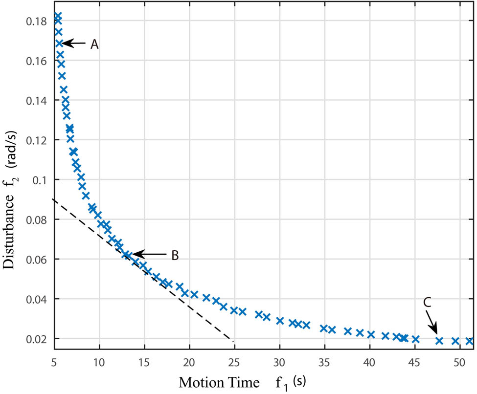
Distribution of non-dominated solutions.

It can be seen that the obtained Pareto frontier curve is in good shape, all non-dominated solutions are located on the curve or very close, and the distribution of points is relatively uniform. This can verify the effectiveness of the improved multi-objective fruit fly algorithm. The contradiction between the two optimization objectives can be seen more intuitively by the curve. Therefore, it is necessary to select typical solutions for detailed comparative analysis.

As marked in Figure 7, three representative non-dominated solutions, A, B, and C, are selected. Point A is the optimal solution for the motion time; point B is the solution where the slope of the tangent of the Pareto curve is 1, that is, the non-dominated solution when the weight of the base attitude disturbance and the motion time are equal; point C is the optimal solution for the base attitude disturbance. The decision variables and optimization target values of the three points are shown in Table 1.

Table 1

Variables and objective function values of typical solutions

Num	v _cs (m/s)	a _cs (m/s)	v _cd (m/s)	a _cd (m/s)	Motion time (s)	Attitude disturbance (rad/s)
A	0.495	0.35	0.506	0.281	5.54	0.169
B	0.143	0.209	0.122	0.169	12.84	0.062
C	0.0367	0.0113	0.0263	0.0108	51.04	0.019

The following is a detailed analysis of the motion process of the capture arm under these three conditions. Since the synchronization constraints have been satisfied in the optimization process, the motion processes of the two capture arms are similar. Change process of the joint angle, angular velocity, and base angular velocity of the single-arm system is given here.

First of all, it can be seen from Figures 8 and 9 that under these three conditions, the joint angle and angular velocity curves are continuous, and the change trends are relatively similar, which indicates that all these three conditions are valid. The difference is that the maximum value of the joint angular velocity decreases as the movement time increases, which is one of the factors that determines the final solution.

Figure 8

Joint angle curves under three conditions. (a) Condition A, (b) condition B, and (c) condition C.

Figure 9

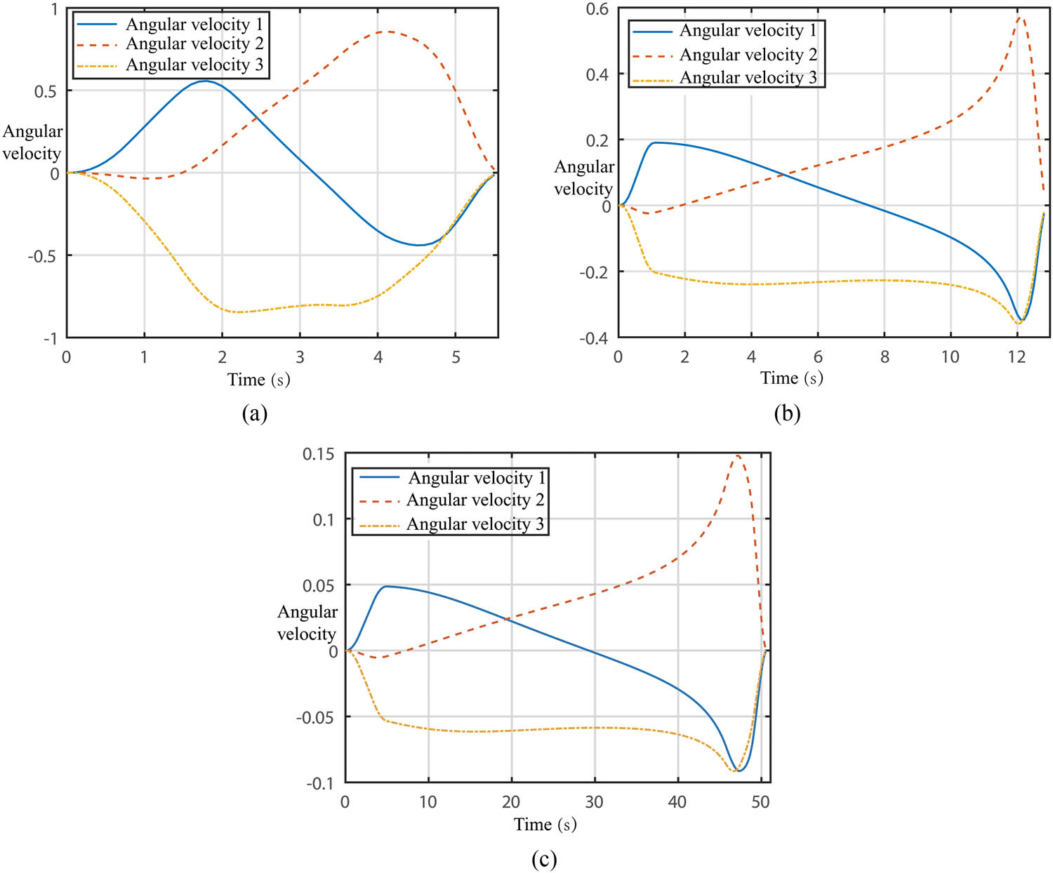
Joint angular velocity curves under three conditions. (a) Condition A, (b) condition B, and (c) condition C.

Through the detailed analysis of the three sets of non-dominated solutions, it can be concluded that the results obtained by the planning method proposed above are all feasible and effective, and the required optimal solution can be selected comprehensively with consideration of time, joint performance, and the disturbance toleration of the base. For example, if the disturbance toleration of the base is strict, while the limit of time is loose, condition C is the preferred solution.

Furthermore, taking condition B as an example, import the data calculated by Matlab into the Adams software to run the simulation, and intercept the states of several time nodes, as shown in Figure 10. It can be seen that the motion synchronization of the two capture arms is good, they can reach the corresponding capture point according to the required configuration. This result can support the effectiveness of the proposed coordination planning strategy strongly.

Figure 10

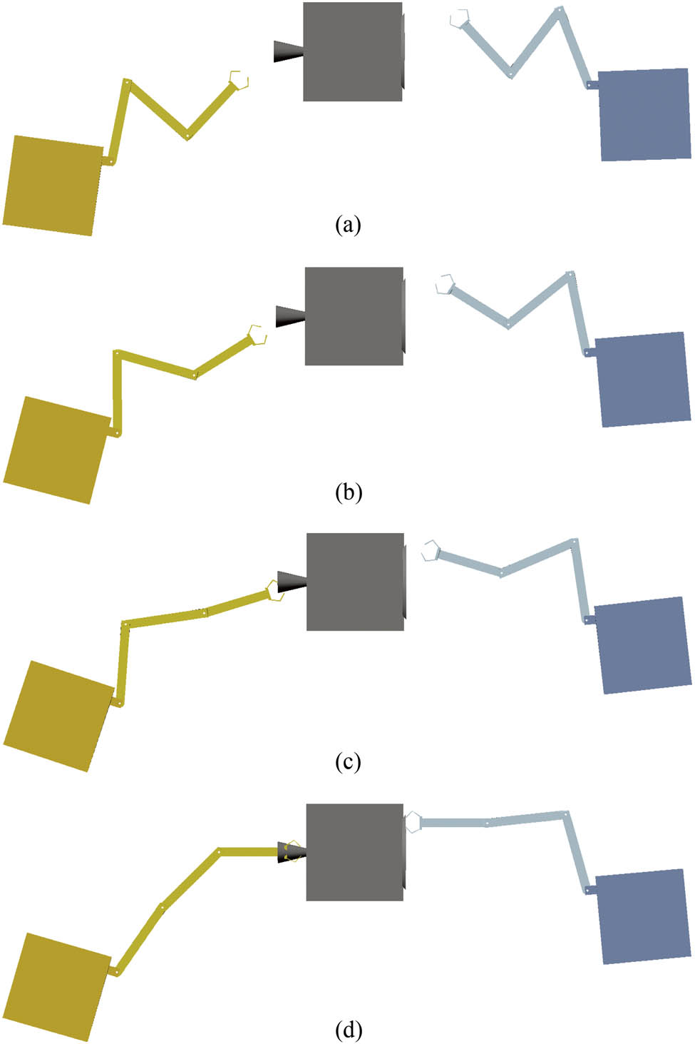
Motion process of the capture system under condition B. (a) 3 s, (b) 6 s, (c) 9 s, and (d) final.

7 Conclusion

First, combining the smoothness of the trapezoidal velocity interpolation and the unity of the drive-transform method, a trajectory planning method based on the trapezoidal velocity interpolation is proposed. Second, a multi-objective optimal model is established to describe the cooperative capture problem, with consideration of the performance of motion time and attitude disturbance. Based on all the above, an improved multi-objective fruit fly algorithm with dual populations is proposed. Finally, typical simulation is carried out. Simulation indicates that the cooperative capture problem can be well solved by the proposed method, and the motion process is smooth, and the different capture arms can reach the target at the same time.

Acknowledgments

This research is funded by the Shanghai Aerospace Science and Technology Innovation Foundation (No. SAST2017-020) and National Key Laboratory Fund for Equipment Pre-research (No. 6142210200301).

Author contributions: All authors have accepted responsibility for the entire content of this manuscript and approved its submission.
Conflict of interest: The authors state no conflict of interest.

References

Boning P, Dubowsky S. 2012. Coordinated control of space robot teams for the on-orbit construction of large flexible space structures. Adv Robot. 24(3):303–323.10.1163/016918609X12619993300665Search in Google Scholar

Chen T. 2021. Continuous leaderless synchronization control of multiple spacecraft on SO(3). Astrodynamics. 5(3):279–291.10.1007/s42064-021-0108-ySearch in Google Scholar

Chen X, Yuan J, Yao W. 2009. Spacecraft on-orbit service technology. Beijing: Aerospace Publishing Press (in Chinese)Search in Google Scholar

Chujo T, Watanabe M, Mori O. 2020. Mechanism-free control method of solar/thermal radiation pressure for application to attitude control. Astrodynamics. 4(3):205–222.10.1007/s42064-019-0062-0Search in Google Scholar

Flores-Abad A, Ma O, Pham K, Ulrich S. 2014. A review of space robotics technologies for on-orbit servicing. Prog Aerosp Sci. 68(8):1–26.10.1016/j.paerosci.2014.03.002Search in Google Scholar

Friend R. 2008. Orbital express program summary and mission overview. Proceedings of the International Society for Optical Engineering Conference. Marseille, France: SPIE. p. 2.10.1117/12.783792Search in Google Scholar

Gao X. 2015. Study on navigation and guidance of formation space robots for rendezvous with non-cooperative target of GEO. Harbin, China: Harbin Institute of Technology (in Chinese)Search in Google Scholar

Lei H. 2020. Dynamical models for secular evolution of navigation satellites. Astrodynamics. 4(1):17–23.10.1007/s42064-019-0064-ySearch in Google Scholar

Liang B, Du X, Li C, Xu W. 2012. Advances in space robot on-orbit servicing for non-cooperative spacecraft. Robot. 34(2):242–256.10.3724/SP.J.1218.2012.00242Search in Google Scholar

Rekleitis G, Papadopoulos E. 2010. Towards passive object on-orbit manipulation by cooperating free-flying robots. Proceedings of International Conference on Robotics and Automation; 2010 May 3–7; Anchorage (AK), USA. IEEE, 2010. p. 2247–2252.10.1109/ROBOT.2010.5509730Search in Google Scholar

Rekleitis G, Papadopoulos E. 2011. On on-orbit passive object handling by cooperating space robotic servicers. Proceedings of International Conference on Intelligent Robots and Systems; 2011 Sep 25–30; San Francisco (CA), USA. IEEE, 2011. p. 595–600.10.1109/IROS.2011.6094858Search in Google Scholar

Rekleitis G, Papadopoulos E. 2013. A comparison of the use of a single large vs a number of small robots in on-orbit servicing. Proceedings of 16th Workshop on Advanced Space Technologies for Robotics and Automation. Noordwijk, Netherlands: ESA. p. 1–6.Search in Google Scholar

Rekleitis G, Papadopoulos E. 2015. On-orbit cooperating space robotic servicers handling a passive object. IEEE T Aero Elec Sys. 51(2):802–814.10.1109/TAES.2014.130584Search in Google Scholar

Wang Y, Chen X, Ran D, Zhao Y, Chen Y, Bai Y. 2020. Spacecraft formation reconfiguration with multi-obstacle avoidance under navigation and control uncertainties using adaptive artificial potential function method. Astrodynamics. 4(1):16–22.10.1007/s42064-019-0049-xSearch in Google Scholar

Wu Z, Yin H, Yan H, Gao Y. 2014. Studies on the collaborative mission planning of multiple space robots based on multiple agent models. Proceedings of 26th Chinese Control and Decision Conference; 2014 31 May–2 June; Changsha, China. IEEE, 2014. p. 4644–4647.10.1109/CCDC.2014.6853002Search in Google Scholar

Yoshida K. 2007. ETS-VII flight experiments for space robot dynamics and control. Berlin Heidelberg: Springer. p. 209–218.10.1007/3-540-45118-8_22Search in Google Scholar

Yuan J. 2015. Research on dual robots manipulating flexible beam on-orbit cooperatively. Harbin, China: Harbin Institute of Technology (in Chinese).Search in Google Scholar

Zhai G, Zhang J, Zhang Y. 2013. Co-loclization of non-cooperative targets based on multiple space robot system. Robot. 35(2):249–256.10.3724/SP.J.1218.2013.00249Search in Google Scholar

Zhai G, Zhang J-R, Zhou Z. 2014. Coordinated localization method for cooperative target based on clustered space robot system. Trans Beijing Inst Technol. 34(10):1034–1039.Search in Google Scholar

Received: 2022-06-30

Revised: 2022-09-06

Accepted: 2022-09-07

Published Online: 2022-12-21

This work is licensed under the Creative Commons Attribution 4.0 International License.

Articles in the same Issue

https://doi.org/10.1515/astro-2022-0198

Keywords for this article

space robots; cooperative capture; fruit fly algorithm; trajectory planning

Creative Commons

BY 4.0