Deep learning application for stellar parameters determination: I-constraining the hyperparameters

1 Introduction

Machine learning (ML) applications have been used extensively in astronomy over the last decade (Baron 2019). This is mainly due to the large amount of data that are recovered from space and ground-based observatories. There is therefore a need to analyse these data in an automated way. Statistical approaches, dimensionality reduction, wavelet decomposition, ML, and deep learning (DL) are all examples of the attempts that were performed in order to derive more accurate stellar parameters such as the effective temperature ( T eff ), surface gravity ( log g ), projected equatorial rotational velocity ( v e sin i ), and metallicity ([M/H]) using stellar spectra in different wavelength ranges (Guiglion et al. 2020, Passegger et al. 2020, Portillo et al. 2020, Wang et al. 2020, Zhang et al. 2020, Bai et al. 2019, Kassounian et al. 2019, Fabbro et al. 2018, Gill et al. 2018, Li et al. 2017, Gebran et al. 2016, Paletou et al. 2015a, b). DL is an ML method based on deep artificial neural networks (ANN) that does not usually require a specific statistical algorithm to predict a solution but it is rather learned by experience and thus require a very large dataset (Zhu et al. 2016) for training in order to perform properly.

An overview of the automated techniques used in stellar parameter determination can be found in the study of Kassounian et al. (2019). We will mention some of the recent studies that involve ML/DL. The increase of the computational power and the large availability of predefined optimized ML packages (in e.g. Python, C++, and R) have allowed astronomers to shift from classical techniques to ML when using large data. One of the first trials to derive the stellar parameters using neural networks was carried out by Bailer-Jones (1997). This work demonstrated that networks can give accurate spectral-type classifications across the spectral-type range B2-M7.

Dafonte et al. (2016) presented an ANN architecture that learns the function which can relate the stellar parameters to the input spectra. They obtained residuals in the derivation of the metallicity below 0.1 dex for stars with Gaia magnitude G rvs < 12 mag, which accounts for a number in the order of four million stars to be observed by the radial velocity spectrograph of the Gaia satellite.^[1] Ramírez Vélez et al. (2018) used an ML algorithm to measure the mean longitudinal magnetic field in stars from polarized spectra of high resolution. They found a considerable improvement of the results, allowing us to estimate the errors associated with the measurements of stellar magnetic fields at different noise levels.

Parks et al. (2018) developed and applied a convolutional neural network (CNN) architecture using multi-task learning to search for and characterize strong HI Ly α absorption in quasar spectra. Fabbro et al. (2018) applied a deep neural network architecture to analyse both SDSS-III APOGEE DR13 and synthetic stellar spectra. This work demonstrated that the stellar parameters are determined with similar precision and accuracy to the APOGEE pipeline.

Sharma et al. (2020) introduced an automated approach for the classification of stellar spectra in the optical region using CNN. They also showed that DL methods with a larger number of layers allow the use of finer details in the spectrum, which results in improved accuracy and better generalization with respect to traditional ML techniques.

Wang et al. (2020) introduced a DL method, SPCANet, which derived T eff and log g and 13 chemical abundances for LAMOST Medium-Resolution Survey data. These authors found abundance precision up to 0.19 dex for spectra with a signal-to-noise ratio (SNR) down to ∼ 10 . The results of SPCANet are consistent with those from other surveys, such as APOGEE, GALAH, and RAVE, and are also validated with the previous literature values including clusters and field stars. Guiglion et al. (2020) derived the atmospheric parameters and abundances of different species for 420165 RAVE spectra. They showed that CNN-based methods provide a powerful way to combine spectroscopic, photometric, and astrometric data without the need to apply any priors in the form of stellar evolutionary models.

More recently, Landa and Reuveni (2021) introduced a multi-layer CNN to forecast solar flare events probability occurrence of M and X classes. Chen et al. (2021) introduced an AGN recognition method based on deep neural network. Almeida et al. (2021) used ML methods to generate model special entry distributions (SEDs) and fit sparse observations of low-luminosity active galactic nuclei. Rhea et al. (2020), Rhea and Rousseau-Nepton (2021) used CNNs and different ANNs to estimate emission-line parameters and line ratios present in different filters of SITELLE spectrometer. Curran et al. (2021) used DL combined with k-Nearest Neighbour and Decision Tree Regression algorithms to compare the accuracy of the predicted photometric redshifts of newly detected sources. Ofman et al. (2022) applied the ThetaRay Artificial Intelligence algorithms to 10,803 light curves of threshold crossing events and uncovered 39 new exoplanetary candidate targets. Bickley et al. (2021) reached a classification accuracy of 88% while investigating the use of a CNN for automated merger classification. Gafeira et al. (2021) used an assisted inversion techniques based on CNN for solar Stokes profile inversions. In the context of classification of galactic morphologies, Gan et al. (2021) used ML generative adversarial networks to convert ground-based Subaru Telescope blurred images into quasi Hubble Space Telescope images. Garraffo et al. (2021) presented StelNet, a deep neural network trained on stellar evolutionary tracks that quickly and accurately predict mass and age from absolute luminosity and effective temperature for stars of solar metallicity.

In this manuscript, we present both a new method to derive stellar atmospheric parameters, and we also demonstrate the effect of each of the CNN parameters (such as the choice of the optimizers, loss function, and activation function) on the accuracy of the results. We will provide the procedure that can be followed in order to find the most appropriate configuration independently of the architecture of the CNN. This is intended as the first in a series of papers that will help the astronomical community to understand the effect on the accuracy of the prediction from most of the parameters and the architecture of the network. CNN parameters are numerous and to find the optimal ones is a very hard task. To do so, we trained the CNNs with different configurations of the parameters using purely synthetic spectra for the three steps of training, cross-validation (hereafter called validation), and testing. Using synthetic spectra, we have access to the true parameters during our tests. Noisy spectra are tested in order to mimic observations.

We have limited our work to a specific type of objects, A stars, because as mentioned previously the purpose is not to show how well we can derive the labelled stellar parameters but what is the effect of specific parameters on stellar spectra analysis. By applying our models to A stars, we use previous results (Gebran et al. 2016, Kassounian et al. 2019) as a reference for the expected accuracy of the derived stellar parameters. In the same way, the wavelength range and the resolving power are chosen to be representative of values used by most available instruments. Once the calibration of the hyperparameters was performed, we have tested our optimal network configurations on a set of FGK stars in Section 6, using the wavelength range of Paletou et al. (2015a).

The training, validation, and test data are explained in Section 2. Section 3 discusses the data preparation previous to training. The neural network construction and the parameter selection are explained in Section 4. Results are summarized in Section 5. The application of the optimal networks to FGK stars is performed in Section 6. Discussion and conclusion are gathered in Section 7.

2 Training spectra

Our learning or training databases (TDB) are constructed from synthetic spectra for stars having effective temperature between 7,000 and 10,000 K, and the wavelength range of 4,450–5,000 Å. This range was selected because it is in the visible domain and contains metallic and Balmer lines sensitive to all stellar parameters ( T eff , log g , [M/H], v e sin i ), especially for the spectra types selected in this work. This region is also insensitive to microturbulent velocity which was adopted to be ξ t = 2 km/s based on the work of Gebran et al. (2016, 2014). Surface gravity, log g , is selected to be in the range of 2.0–5.0 dex. Projected rotational velocity, v e sin i , is calculated between 0 and 300  km s − 1 . The metallicity, [M/H], is in the range of − 1.5 and +1.5 dex. Table 1 displays the range of all stellar parameters. These spectra are used for both the training and the validation phases. Approximately 55,000 noise free synthetic spectra were calculated using a random selection of the stellar parameters in the range of Table 1. These spectra are used instead of the observations (test data without noise). Gaussian SNRs, ranging between 5 and 300, were added to these test spectra in order to check the accuracy of the technique on noisy data (test data with noise).

Details for the calculations of the synthetic spectra can be found in the study of Gebran et al. (2016) or Kassounian et al. (2019). In summary, 1D plane-parallel model atmospheres were calculated using ATLAS9 (Kurucz 1992). These models are in local thermodynamic equilibrium (LTE) and in hydrostatic and radiative equilibrium. We have used the new opacity distribution function in the calculations (Castelli and Kurucz 2003) as well as a mixing length parameter of 0.5 for 7,000 K ≤ T eff ≤ 8,500 K , and 1.25 for T eff ≤ 7,000 K (Smalley 2004).

We have used Hubeny and Lanz (1992) SYNSPEC48 synthetic spectra code to calculate all normalized spectra. The adopted line lists are detailed in the study of Gebran et al. (2016). This list is mainly compiled using the data from Kurucz gfhyperall.dat^[2], VALD^[3], and the NIST^[4] databases.

Finally, the resolving power is simulated to R = 60,000 . This value falls in the range between low and high resolution spectrographs. The technique that will be shown in the next sections can be used for any resolution. The construction and the size of the TDB will be discussed in Section 5. The use of synthetic spectra in ML to constrain the stellar parameters has shown to suffer from the so-called synthetic gap (Fabbro et al. 2018, Passegger et al. 2020). This gap refers to the differences in feature distributions between synthetic and observed data. We have decided to limit our work to synthetic data for two reasons: first we would like to remove the hassle of the data preparation steps (data reduction, flux calibration, flux normalization, radial velocity correction, and so on), and second because our intention is to find the strategy and technique that should be adopted in ML for deriving stellar parameters.

We are working on a future paper that deals with the architecture of the network as well as the choice of the kernel sizes and the number of neurons. Combining the best strategy to constrain the hyperparameters (this manuscript) as well as the most optimal architecture (future studies) will allow us to use a combination of synthetic and observational data in our training database. Having well-known stellar parameters, these observational data will allow us to remove/minimize the synthetic gap and better constrain the stellar parameters.

3 Data preparation

The TDB contains N spectra spectra that span the wavelength range of 4,450–5,000 Å. Having a wavelength step of 0.05 Å, this results in N λ = 10,800 flux points per spectrum. The TDB can then be represented by a matrix M of size N spectra × N λ . A colour map of a subsample of M is displayed in Figure 1. Although the synthetic spectra are normalized, some wavelength points could have fluxes larger than unity. This is due to the noise that is incorporated during the so-called data augmentation procedure, which will be explained in Section 4.1.1.

Figure 1

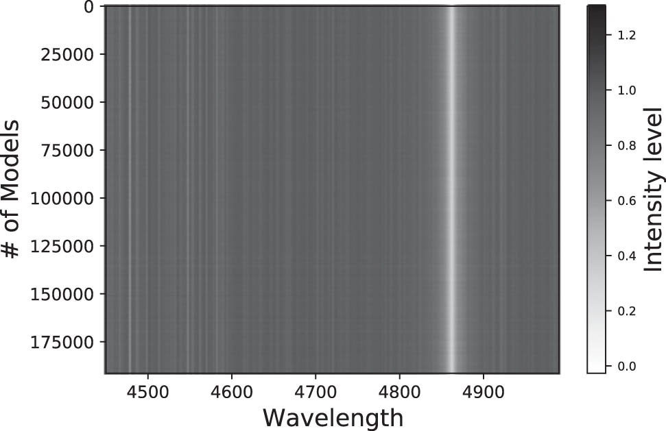
Colour map representing the fluxes for a sample of the training database using data augmentation. Wavelengths are in Å.

Training a CNN using the M matrix is time consuming, especially if one should use a larger wavelength range or a higher resolution. For that reason, we have applied a dimensionality reduction technique, i.e. principal component analysis (PCA), in order to reduce the size of the training TDB as well as the size of the validation, test, and noisy synthetic data. Although this step is optional, we recommend its use whenever the data can be represented by a small number of coefficients. The PCA can reduce the size of each spectrum from N λ to n k . The choice of n k depends on the many parameters, the size of the database, the wavelength range, and the shape of the spectra lines. As a first step, we need to find the principal components, and to do so, we proceed as follows.

The matrix M is averaged along the N spectra -axis and the result is stored in a vector M ¯ . Then, we calculate the eigenvectors e k ( λ ) of the variance–covariance matrix C defined as

where the superscript “T” stands for the transpose operator. C has a dimension of N λ × N λ . Sorting the eigenvectors of the variance–covariance matrix in decreasing magnitude will result in the “principal components.” Each spectrum of M is then projected on these principal components in order to find its corresponding coefficient p j k defined as

The choice of the number of coefficient is regulated by the reconstructed error as detailed in the study of Paletou et al. (2015a):

We have opted to a value for n k that reduces the mean reconstructed error to a value of < 0.5 % . As an example, using a database of 25,000 spectra with stellar parameters ranging randomly between the values in Table 1 requires less than seven coefficients to reach an accuracy < 1 % , and a value of n k = 17 to reach a 0.5% error as shown in Figure 2. This technique has shown its efficiency when applied to synthetic and/or real observational data with T eff > 4,000 K (see Gebran et al. 2016, Paletou et al. 2015a, b, for more details).

Figure 2

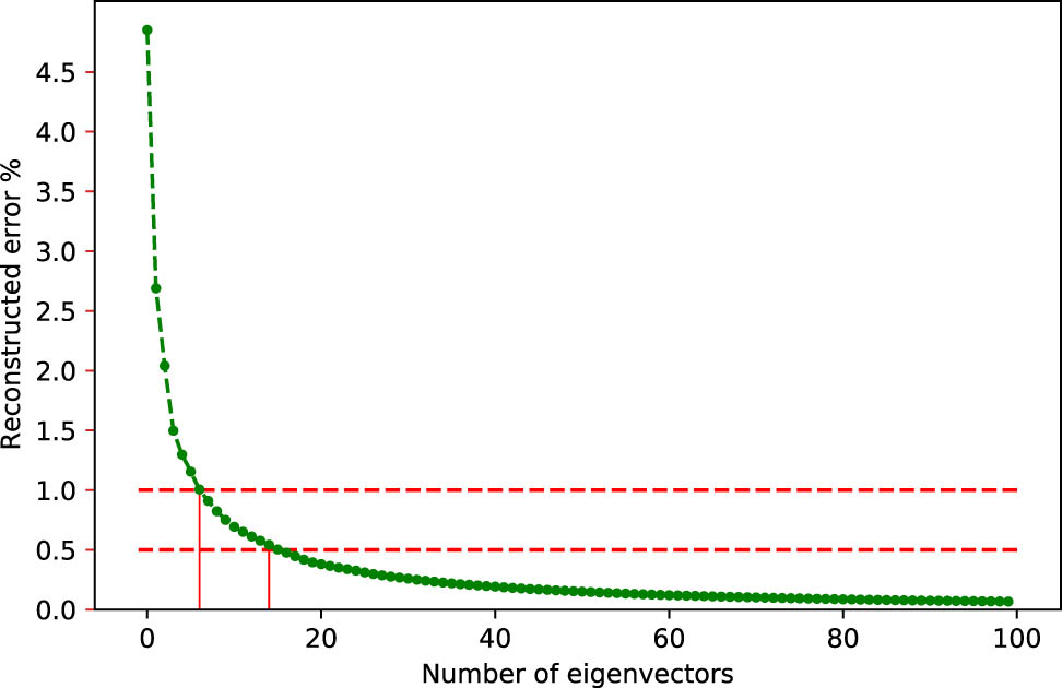
Mean reconstructed error as a function of the number of principal components used for the projection. The dashed lines represent the 1 and 0.5% error, respectively. For n k > 17 , the spectra can be reconstructed with more than 99.5% accuracy.

Applying the same procedure to all our TDB and taking the maximum value to be used for all, we have adopted a constant value for n k = 50 . This value takes into account all the databases that will be dealt with in this work, especially that some will be data augmented as will be explained in Section 4.1.1. This means that instead of training a matrix having a dimension of N spectra × N λ , we are using one with dimension of N spectra × n k , with n k ≪ N λ . In that case, our new data consist of a matrix containing the coefficients that are calculated by projecting the spectra on the n k eigenvectors.

This projection procedure over the principal components is then applied to the validation, test, and noisy spectra datasets.

4 DL: ANN

This section begins with a brief description of supervised^[5] learning. Given a data set ( X , Y ) , the goal is to find a function f such that f ( X ) is as “close” as possible to Y . For example, Y could be the effective temperature or surface gravity and X the corresponding spectra. This “closeness” is typically measured by defining a loss function L ( f ( X ) , Y ) that measures the difference between the predicted and actual values. Therefore, the goal of the learning process is to find f that minimizes L for a given dataset ( X , Y ) . Ultimately, the success of any learning method is assessed by how well it generalizes. In other words, once the optimal f is found for the training set ( X , Y ) , and given another data set ( U , V ) , how close is f ( U ) to V .

One of the most successful methods in tackling this kind of problem is ANN, a subset of ML. As the name suggests, an ANN is a set of connected building blocks called neurons which are meant to mimic the operations of biological neurons (Anthony and Bartlett 1999, Wang 2003). Different kinds of ANNs can be built by varying the number of connections between and operations of individual neurons. The operations performed by these neurons depend on a number of parameters called weights and some nonlinear function called the activation. At a high level, an ANN is just the function f that was described earlier. Since the network architecture is chosen at the start, finding the optimal f boils down to finding the optimal weight parameters that minimize the cost function L .

Regardless of the type of ANN used, the process of finding the optimal weights is more or less the same, and works as follows. After the network architecture is chosen, the weights are initialized, then a variant of gradient descent is applied to the training data. Gradient descent changes the parameters iteratively, at a certain rate proportional to their gradient, until the loss value is sufficiently small (Ruder 2016). The proportionality constant is called the learning rate. While this process is well-known, there is to date no clear prescription for the choice of different components. The main difficulty arises from the fact that the loss function contains multiple minima with different generalization properties. In other words, not all minima of the loss function are equal in terms of generalization. Which minimum is reached at the end of training phase depends on the initial values chosen for the weights, the optimization algorithm used, including the learning rate and the training dataset (Zhang et al. 2016). In the absence of clear theoretical prescriptions for the components, one has to rely on experience and best practices (Bengio 2012).

One popular type of ANN is the feedforward network, where neurons are organized in layers, with the outputs of each layer fully connected to the inputs of the next. By increasing the number of layers (whence the “deep” in “DL”), many types of data can be modelled to a high degree of accuracy. Fully connected ANNs, however, have some shortcomings, such as the large number of parameters, slow convergence, overfitting, and most importantly, failure to detect local patterns. Almost all the aforementioned shortcomings are solved by using convolution layers.

4.1 CNN

A CNN is a multi-layer network where at least one of the layers is a convolution layer LeCun (1989). As the name suggests, the output of a convolution layer is the result of a convolution operation, rather than matrix multiplication, as in feedforward layers, on its input. Typically, this convolution operation is performed via a set of filters. CNNs have been very successful in image recognition tasks (Yim et al. 2015). Most commonly, CNNs are used in conjunction with pooling layers. In this work, since the input to the CNN has been already processed with PCA to reduce the dimension of the training database, we decided to omit pooling layers in our work. Even though CNNs have been mostly used for processing image data, which can be viewed as 2D grid data, they can also be used for 1D data as well.

The architecture of a CNN differs among various studies. There is no perfect model, it all depends on the type and size of the input data, and on the type of the predicted parameters. In this work, we will not be constraining the architecture of the model but rather we will be providing the best strategy to constrain the parameters of the model for a specific and defined architecture. Figure 3 shows a flow chart of a typical CNN. Table 2 represents the different layers, the output shape for each layer, and the number of parameters used in our model. In the same table, “Conv” stands for convolutional layer, “Flat” for flattening layer which transforms the matrix of data to one dimensional, and “Full” stands for fully connected layer. The total number of parameters to be trained every iteration is 764,357. The choice of such an architecture is based on aF trial and error procedure that we performed in order to find the best model that can handle all types of training databases used in this work. The strategy of selecting the number of hidden layers and the size of the convolution layers will be described in a future paper. We decided to do all our tests using the ML platform TensorFlow ^[6] with the Keras ^[7] interface. The reason is that these two options are open-source and written in Python.

Figure 3

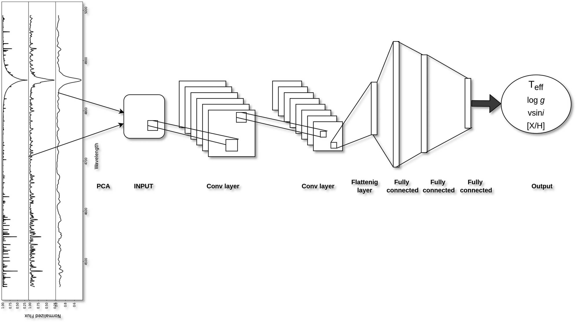
CNN architecture used in this work. A PCA dimension reduction transforms the spectra into a matrix of input coefficient. This input passes through several convolutional layers and fully connected layers in order to train the data and predict the stellar parameters.

Table 2

Different layers that are used in the CNN used in our work

Layer	Output shape	# Parameters
Conv	50 × 8	40
Conv	50 × 4	132
Conv	50 × 4	68
Flat	200	0
Full	1,024	205,824
Full	512	524,800
Full	64	32,832
Full	10	650
Full	1	11

Although the calculation time is an important parameter constraining the choice of a network, we have decided not to take it into consideration while selecting the optimal network. The reason for that is that the calculation time depends mainly on the network’s architecture which is not discussed in this article. Two parameters are also constraining the calculation time, the number of epochs, and the batch size (related to the size of the TDB). Calculation time increases with increasing epoch number and decreases with increasing batch size. The main goal of this work is to find the optimal configuration for the parameters independently of the calculation time and the Network architecture. As a rule of thumb, using a Database of 70,000 spectra and 50 eigenvectors, it takes around 17 h to run the CNN over 2,000 epochs using 64 batches and a Dropout of 30%. These calculations are done on a Intel Core i7-8750H CPU @ 2.20 GHz × 6 CPU.

4.1.1 Data augmentation

Data augmentation is a regularization technique that increases the diversity of the training data by applying different transformations to the existing one. It is usually used for image classification (Shorten and Khoshgoftaar 2019) and speech recognition (Jaitly and Hinton 2013). We tested this approach in our procedure in order to take into account some modifications that could occur in the shape of the observed spectra due to a bad normalization or inappropriate data reduction. We also took into account the fact that observed spectra are affected by noise and that the learning process should include the effect of this parameter.

For each spectrum in the TDB, five replicas were performed. Each of these five replicas has different amount of flux values but they all have the same stellar labels T eff , log g , [M/H], and v e sin i . The modifications are done as follows:

1. A Gaussian noise is added to the spectrum with an SNR ranging randomly between 5 and 300.

2. The flux is multiplied in a uniform way with a scaling factor between 0.95 and 1.05.

3. The flux is multiplied with a new scaling factor and noise was added.

4. The flux is multiplied by a second-degree polynomial with values ranging between 0.95 and 1.05 and having its maximum randomly selected between 4,450 and 5,000 Å.

5. The flux is multiplied by a second-degree polynomial and Gaussian noise added to it.

The purpose of this choice is to increase the dimension of the TDB from N spectra × N λ to 6 × N spectra × N λ and to introduce some modifications in the training spectra that could appear in the observations that we need to analyse. Such modifications are the noise and the commonly observed departures from a perfect continuum normalization. Distortions in observed spectra could appear due to bad selection in the continuum points. We have tested the two options, with and without data augmentation, and the results are shown in Section 5. Figure 4 displays one synthetic spectrum having T eff = 8,800 K , log g = 4.0 dex, v e sin i = 14 km s − 1 , and [M/H] = 0.0 dex as well as the extra five modifications that were performed on this spectrum. We have decided to use a continuous SNR between 5 and 300 but different modifications could be tested. As an example, González-Marcos et al. (2017) adapted the SNR of the spectra used in the training dataset to the SNR of the spectra for which the atmospheric parameters are needed (evaluation set). They concluded that in case of T eff , only two regression models are needed (SNR = 50 and 10) to cover the entire SNR range.

Figure 4

The effect of the data augmentation on the shape of the spectra. Upper left: spectrum represents the original synthetic spectra. Upper middle: Gaussian noise added to the synthetic spectra. Upper right: synthetic spectrum with the intensities multiplied by a constant scale factor. Bottom left: Gaussian noise added to the synthetic spectra and multiplied by a constant scale factor. Bottom middle: synthetic spectrum with the intensities multiplied by a second-degree polynomial. Bottom right: Gaussian noise added to the synthetic spectra and multiplied by a second-degree polynomial. All these spectra have the same stellar parameters ( T eff = 8,800 K , log g = 4.3 dex, v e sin i = 45 km s − 1 , [M/H] = 0.0 dex).

4.1.2 Initializers: Kernel and bias

The initialization defines the way to set the initial weights. There are various ways to initialize, and we will be testing the following:

1. Zeros: weights are initialized with 0. In that case, the activation in all neurons is the same and the derivative of the loss function is similar for every weight in every neuron. This results in a linear behaviour for the model.

2. Ones: a similar behaviour as the Zeros but using the value of 1 instead of 0.

3. RandomNormal: initialization with a normal distribution.

4. RandomUniform: initialization with a uniform distribution.

5. TruncatedNormal: initialization with a truncated normal distribution.

6. VarianceScaling: initialization that adapts its scale to the shape of weights.

7. Orthogonal: initialization that generates a random orthogonal matrix.

8. Identity: initialization that generates the identity matrix.

9. Lecun_uniform: LeCun uniform initializer (Lecun et al. 1998).

10. Glorot_normal: Xavier normal initializer (Glorot and Bengio 2010).

11. Glorot_uniform: Xavier uniform initializer (Glorot and Bengio 2010).

12. he_normal: He normal initializer (He et al. 2015).

13. Lecun_normal: LeCun normal initializer (Lecun et al. 1998).

14. he_uniform: He uniform variance scaling initializer (He et al. 2015).

For all of these initializers, the biases are initialized with a value of zero. It will be shown later that most of these initializers give the same accuracy except for the zeros and ones.

4.1.3 Optimizer

Once the (parameterized) network architecture is chosen, the next step is to find the optimal values for the parameters. If we denote by θ the collective set of parameters, then, by definition, the optimal values, θ ∗ , are the ones that minimize a certain loss function L ( θ ) ; a measure of difference between the predicted and the actual values. This optimization problem is, typically, solved in an iterative manner, by computing the gradient of the loss function with respect to the parameters.

Let θ t denote the set of parameters at iteration t. The iterative optimization process produces a sequence of values, θ 1 , … , θ ∗ that converges to the optimal values θ ∗ . At a given step t we define the history of that process as the set ℋ t = { θ i , L ( θ i ) , ∇ L ( θ i ) } i = 0 t . The values θ t + 1 are obtained from θ t according to some update rule U

(4) θ t + 1 = U ( H t , γ t ) ,

where γ t is a set of hyperparameters such as the learning rate.

Different optimization techniques use a different update rule. For example, in the so-called “vanilla” gradient descent, the update rule depends on the most recent gradient only:

(5) θ t + 1 = θ t − γ ∇ L ( θ t ) .

Other methods include the whole history with different functional dependence on the gradient and different rates for each step (see Choi et al. 2020 for a survey). Different optimization techniques are available in keras and we will be testing the following:

1. Adam: an adaptive moment estimation that is widely used for problems with noise and sparse gradients. Practically, this optimizer requires little tuning for different problems.

2. RMSprop: a root mean square propagation that iteratively updates the learning rates for each trainable parameter by using the running average of the squares of previous gradients.

3. Adadelta: it is an adaptive delta, where delta refers to the difference between the current weight and the newly updated weight. It also works as a stochastic gradient descent method.

4. Adamax: an adaptive stochastic gradient descent method and a variant of Adam are based on the infinity norm. It is also less sensitive to the learning rates than other optimizers.

5. Nadam: Nesterov-accelerated Adam optimizer that is used for gradients with noise or with high curvatures. It uses an accelerated learning process by summing up the exponential decay of the moving averages for the previous and current gradient. It is also an adaptive learning rate algorithm and requires less tuning of the hyperparameters.

4.1.4 Learning rate

As mentioned in the beginning of the section the training rate can affect the minimum reached by the loss function and therefore has a large effect on the generalization property of the solution. In this article, we followed the recommendation of Bengio (2012) and chose the learning rate value to be half of the largest rate that causes divergence.

4.1.5 Dropout

Dropout is a regularization technique for neural networks and DL models that prevent the network from overfitting (Srivastava et al. 2014). When dropout is applied, randomly selected neurons removed each iteration of the training and do not contribute to the forward propagation and no weight updates are applied to these neurons during backward propagation. Statistically, this has the effect of doing ensemble average over different sub-networks obtained from the original base network. We tried to find the optimal number for the dropped out fraction of neurons. Dropout layers are put after each convolutional one. Tests were performed with dropout fraction ranging between 0 and 1.

4.1.6 Pooling

Pooling layer is a way to down sample the features (i.e. reducing the dimension of the data) in the database by taking patches together during the training. The most common pooling methods are the average and the max pooling Zhou and Chellappa (1988). The average one summarizes the mean intensity of the features in a patch and the max one considers only the most intense (i.e. highest value) value in a patch. The size of the patches and the number of filters used are decided by the user. The standard way to do that is to add a pooling layer after the convolutional layer and this can be repeated one or more times in a given CNN. However, pooling makes the input invariant to small translations. In image detection, we need to know if the features exist and not their exact position. That is why this technique has shown to be valuable when analysing images (Goodfellow et al. 2016). This is not the case in spectra because the position of the lines needs to be well-known (Section 5). But also, as discussed previously, pooling layers are not needed in our case because the dimension of the TDB was already reduced drastically by applying PCA.

4.1.7 Activation functions

The activation function is a non linear transformation that is applied on the output of a layer and this output is then sent to the next layer of neurons as input. Activation functions play a crucial role in deriving the output of a model, determining its accuracy and computational efficiency. In some cases, activation functions might prevent the network from converging.

The activation function for the inner layers of deep networks must be nonlinear, otherwise no matter how deep the network is, it would be equivalent to single layer (i.e. regression/logistic regression). Having said that we have tested five activation functions that are as follows:

1. sigmoid: f ( x ) = 1 1 + e − x

2. tanh: f ( x ) = e x − e − x e x + e − x

3. relu: f ( x ) = Max ( 0 , x )

4. elu: f ( x ) = x x ≥ 0 α ( e x − 1 ) x < 0

5. selu: f ( x ) = λ x x ≥ 0 λ α ( e x − 1 ) x < 0 .

It is important to note that in this section we discuss the choice of the activation function for inner layers only. The choice of the activation for the last layer is usually more or less fixed by the type of the problem and how one is modelling it. For example, if one is performing binary classification, then a sigmoid-like activation is usually used (or softmax for multiclass classification) and interpreted as a probability. However, for regression-like problems a linear activation is usually used for the last layer. In our case, which is a purely regression problem, the last layer will have a linear activation function.

The sigmoid and tanh restrict the magnitude of the output of the layer to be ≤ 1 . Both, however, suffer from the vanishing gradient problem (Glorot et al. 2011). For relatively large magnitudes both functions saturate and their gradient becomes very small. Since deep networks rely on backpropagation for training the gradient, the first few layers, being a product of the succeeding layers, become increasingly small. The rectifier class of activation, relu, elu, and so on seem to minimize the vanishing gradient problem. Also, they lead to sparse representation, which seems to give better results (He et al. 2015, Maas 2013).

4.1.8 Loss functions

The loss function controls the prediction error of an NN as explained in Section 4. It is an important criterion in controlling the updates of the weights in an NN, mainly during the backward propagation. The selection of the type of the loss function is decided depending on the types of output labels. If the output is a categorical variable, one can use the categorical crossentropy or the sparse categorical crossentropy. If we are dealing with a binary classification, binary crossentropy will be the normal choice for a loss function. Finally, in case of a regression problem like the one used in stellar spectra parameters determination, variants of mean squared error loss functions are used. In our work, we have tested the following functions:

1. Mean squared error: 1 N ∑ i = 1 N ( y i − y ˆ i ) 2

2. Mean squared logarithmic error: 1 N ∑ i = 1 N ( log 1 + y i 1 + y ˆ i ) 2

3. Mean absolute error: 1 N ∑ i = 1 N ∣ y i − y ˆ i ∣

y being the actual label, y ˆ the predicted ones, and N the number of spectra in the training dataset.

Loss function selection can differ from one study to the other (Rosasco et al. 2004). For that reason, we have tested the above three functions in deriving the stellar parameters.

4.1.9 Epochs

The number of epochs is the number of times the whole dataset is used for the forward and the backward propagation. The number of Epochs controls the number of times the weights of the neurons are updated. While increasing the number of Epochs, we can move from underfitting to overfitting passing through the optimal solution for our network.

4.1.10 Batches

Instead of passing the whole training dataset into the NN, we can divide it in N Batches batches and iterate on all batches per epoch. In that case, the number of iteration will be the number of batches needed to complete one epoch. Batches are used in order to avoid the saturation of the computer memory and the decrease of iterations speed. However, the selection of the optimal batch number is not straightforward. Adopted values are usually 32, 64, or 128 (Keskar et al. 2016).

One of the most important measures of the success for a deep neural network is how well it generalizes on some test data, not included in the training phase. In current deep neural networks, the loss function has multiple minima. Many experimental studies have shown that, during the training phase, the path to reaching a minimum is as important as the final value (Neyshabur et al. 2017, Zou et al. 2019, Zhang et al. 2016). A good rule of thumb is that a “small,” less than 1% the size of the data, batch size generalizes better than “large” batches, about 10% of the training data (Keskar et al. 2016).

5 Results and analysis

The effect of each CNN parameter on the accuracy of the stellar parameters has been tested. To do so, we have used the same CNN with the same parameters for all our tests while changing only the concerned one at each time. For example, to find the best epoch numbers, we fix the activation function, the optimizer, the number of batches, the dropout percentage, the loss function, and the kernel initializer while iterating on the number of epochs. The same parameters are used again for finding the optimal dropout percentage and so on. The fixed values used in these calculations are the he_normal for the kernel initializer, the mean squared error for the loss function, the “ADAM” optimizer, the relu activation function, 50% of dropout, 64 batches. These tests are performed with epochs of 100, 500, 1,000, 2,000, 3,000, 4,000, and 5,000. In all tests, the distribution of Training and Validation is 80% and 20%, respectively.

The results will be a combination of test errors spanning over different number of epochs for each stellar parameter and CNN configuration. The variation with the number of epochs ensures that the trends are real and not due to local minima as a result of the low number of iterations. The tests are a collection of 110,000 synthetic spectra, half of them without noise and half with random noise as introduced in Section 2.

To better visualize the results and to have a better conclusion about the optimal configurations, we display in Figures 5–8 the relative error of the observations. These errors are calculated by dividing the values by the maximum observation standard deviation in all configurations (i.e. including all epoch simulations). This will allow us to target the minimum values and pinpoint the best parameters.

Figure 5

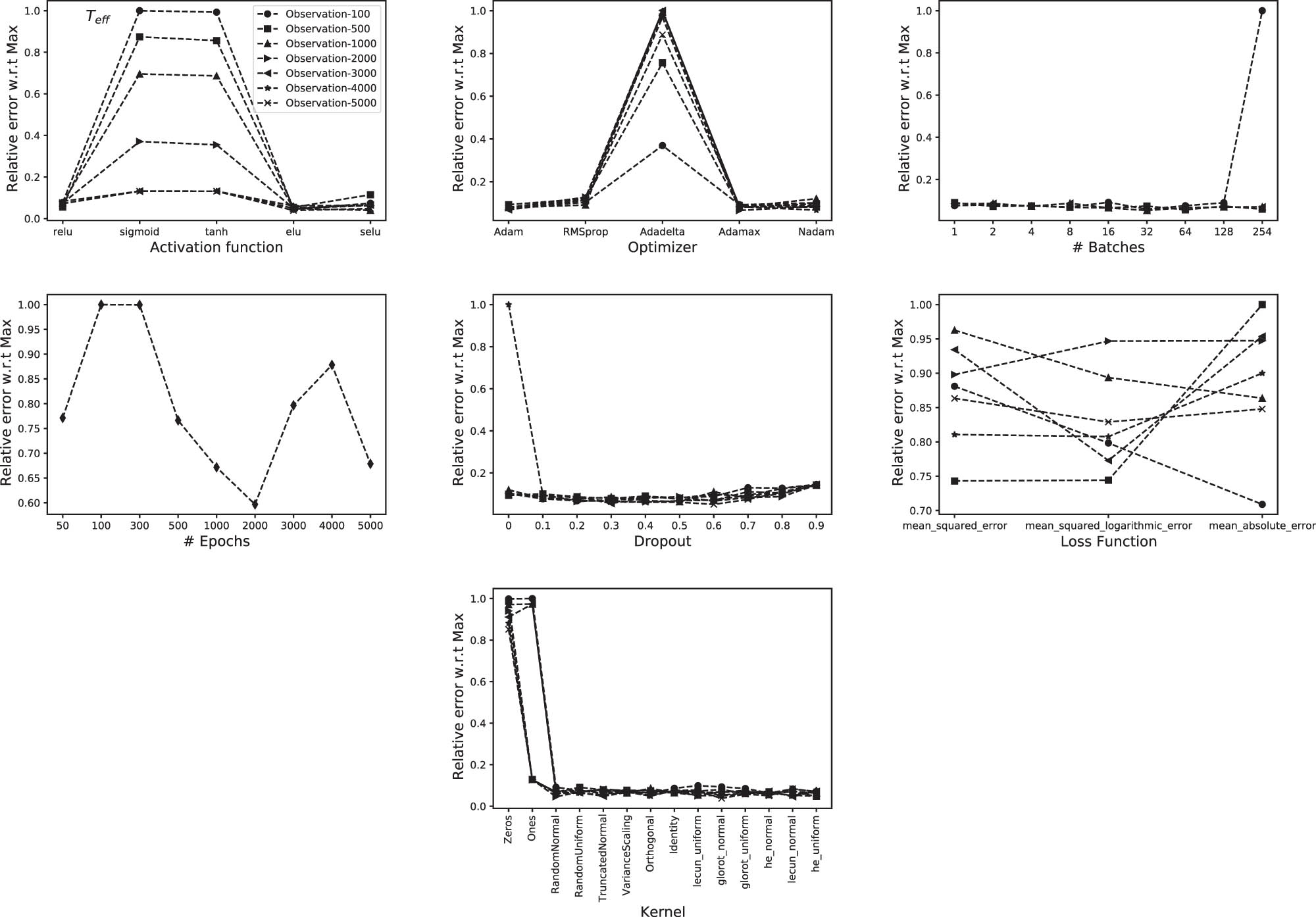
Effect of varying the CNN parameters on the accuracy of T eff for different epoch numbers. The results are displayed by dividing the observation standard deviation by their maximum value in each test.

In what follows, we show the results that were performed using a training dataset of 40,000 randomly generated synthetic spectra in the ranges of Table 1. In Section 5.5, we discuss the effect of using a small or a large training database and the effect of using or not data augmentation.

5.2 Surface gravity

The accuracies for gravity behave differently than the one of T eff with respect to the various parameters. According to Figure 6, the optimal values are found to be relu or tanh for the activation function; Adam, Adamax, or RMSprop for the optimizer, a number of batches between 32 and 128, an epoch number of 3,000, a Dropout fraction between 0.3 and 0.4, a mean squared logarithmic error loss function, and all kinds of initializers except for zeros and ones.

Figure 6

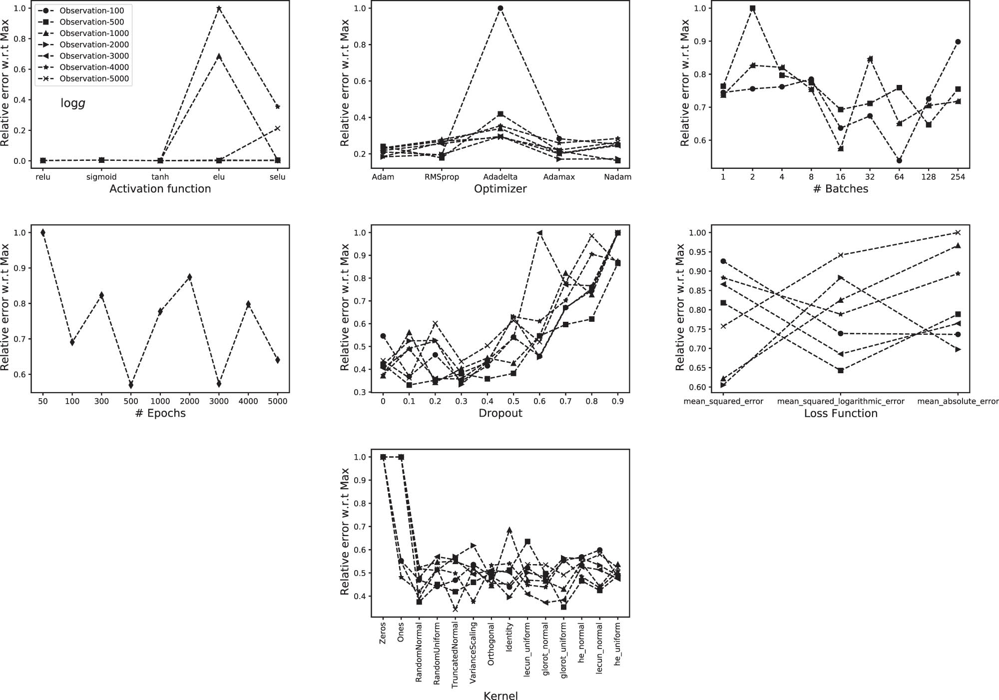
Same as Figure 5 but for log g .

In case of log g the optimal configuration is found to be using the following parameters:

• Activation function: tanh .

• Optimizer: Adamax.

• Batches: 128.

• Epochs: 3,000.

• Dropout: 30%.

• Loss function: mean squared logarithmic error.

• Kernel initializer: he_normal.

5.3 Metallicity

The metallicity parameter, [M/H], also behaves differently than T eff and log g . As seen in Figure 7, [M/H] requires a different combination of parameters in our CNN in order to reach optimal results. tanh or relu activation functions give the least error in most epoch number situations. Adam and RMSprop optimizer lead to similar results within few percents of differences. A combination of 16 batches and 1,000 epochs is appropriate to derive [M/H] with low errors. A dropout between 10 and 30%, a mean absolute error for a loss function, and a RandomUniform kernel initializer are to be used in order to reach the highest possible accuracy for [M/H]. Our technique was applied to A stars and extrapolated to FGK stars (Section 6). However, specific considerations should be taken into account when deriving the metallicities of cool stars due to forests of molecular lines that are present in the spectra (Passegger et al. 2021).

Figure 7

Same as Figure 5 but for [M/H].

In case of [M/H], the optimal configuration is found to be using the following parameters:

• Activation function: tanh .

• Optimizer: Adam.

• Batches: 16.

• Epochs: 1,000.

• Dropout: 20%.

• Loss function: mean absolute error.

• Kernel initializer: RandomUniform.

5.4 Projected equatorial rotational velocity

Finally, in case of the equatorial projected rotational velocity, v e sin i , tanh seems to be the optimal activation function independently of the epoch and batches number (Figure 8). Adam or Adamax optimizers can be used for v e sin i with small differences in the derived accuracies. A combination of 32 batches with 3,000 epochs is the one that gives the minimum error for the derived v e sin i values. A dropout fraction between 0.1 and 0.4 yields very close errors. A mean squared error can be used for the loss function and all kernel initializers can also be applied except the zeros and ones for the same reason explained in Section 5.1.

Figure 8

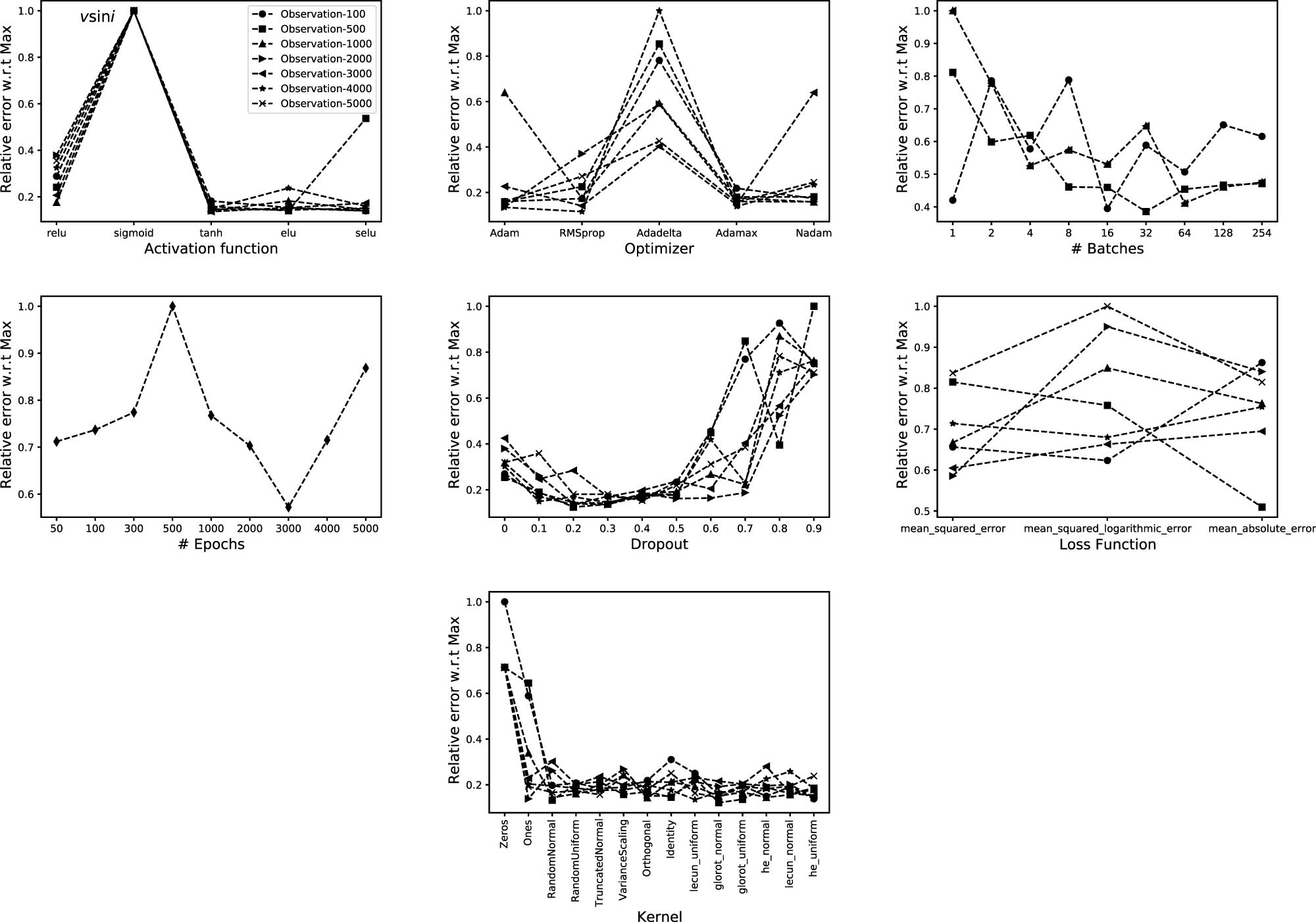
Same as Figure 5 but for v e sin i .

In case of v e sin i , the optimal configuration is found to be using the following parameters:

• Activation function: tanh .

• Optimizer: Adamax.

• Batches: 32.

• Epochs: 3,000.

• Dropout: 30%.

• Loss function: mean squared error.

• Kernel initializer: he_Uniform.

5.5 Database size and the role of augmentation

In order to check the dependency of the performance of the CNN on the size of the training set, three databases are used. The first database (TDB1) contains 25,000 random synthetic spectra as explained in Section 5, the second database (TDB2) contains 40,000 random spectra, and the third (TDB3) contains 70,000 spectra, resulting from the same TDB1 parameter ranges. We have also checked the importance of using Data Augmentation as a regularization technique for deriving accurate parameters (see Section 4.1.1 for details).

For each stellar parameter, we used the optimal CNN with the configuration that was derived in Sections 5.1–5.4. Each configuration was tested with TDB1, TDB2, and TDB3 with and without Data Augmentation. Figure 9 displays the average relative standard deviation for each stellar parameter with respect to the maximum values, for the training, validation, test, and observation sets. In order to quantify these proxies for the uncertainties of the techniques, Table 3 collects the standard deviations for the four stellar parameters as a function of the training database.

Figure 9

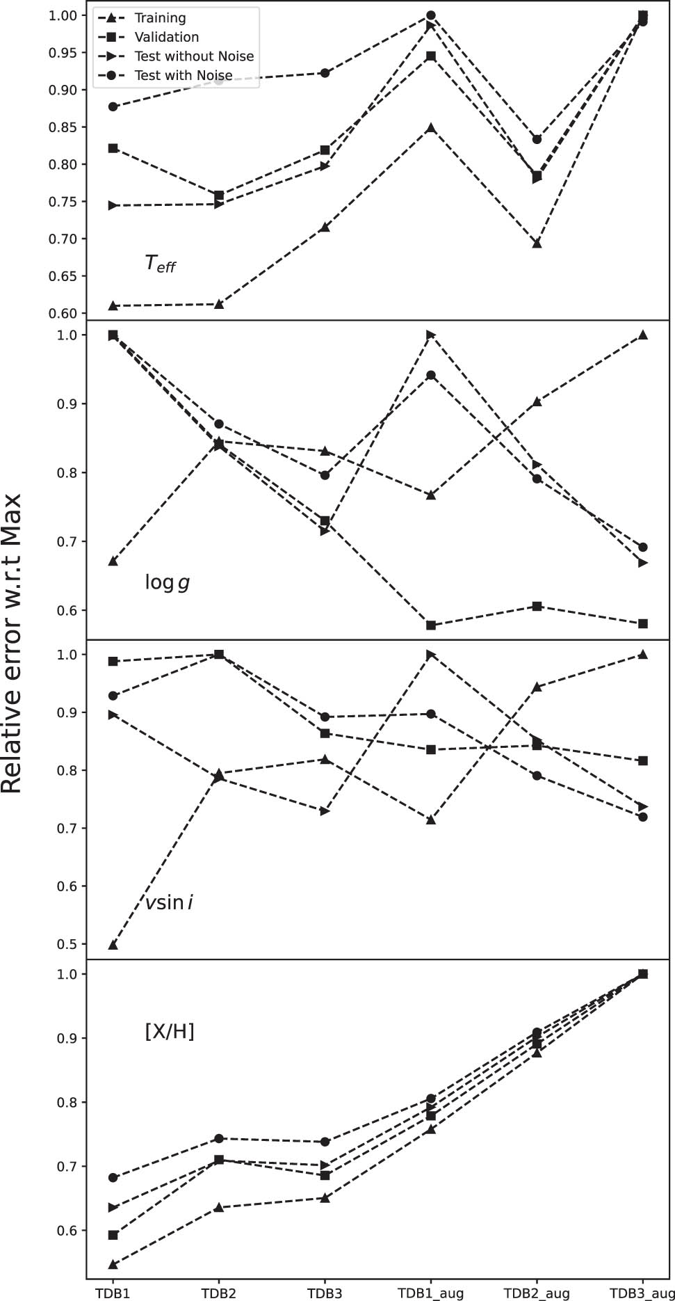
Relative errors for each stellar parameter using TDB1, TDB2, and TDB3 with and without data augmentation as a training dataset.

Table 3

Derived standard deviation for each parameter using TDB1, TDB2, and TDB3 with and without data augmentation

Database	σ T eff (K)	σ log g (dex)	σ [ M/H ] (dex)	σ v e sin i km s − 1
	TDB1
Training	78	0.03	0.06	0.97
Validation	112	0.11	0.07	4.00
Test without noise	98	0.10	0.07	3.30
Test with noise	133	0.13	0.07	5.25
	TDB1 with data augmentation
Training	109	0.03	0.09	1.40
Validation	129	0.07	0.09	3.36
Test without noise	129	0.10	0.10	3.66
Test with noise	152	0.12	0.10	5.00
	TDB2
Training	79	0.04	0.08	1.55
Validation	104	0.10	0.08	4.00
Test without noise	99	0.09	0.09	2.90
Test with noise	139	0.11	0.09	5.50
	TDB2 with data augmentation
Training	89	0.04	0.10	1.85
Validation	107	0.07	0.10	3.40
Test without noise	103	0.09	0.10	3.12
Test with noise	127	0.10	0.11	4.36
	TDB3
Training	92	0.04	0.07	1.60
Validation	112	0.08	0.08	3.50
Test without noise	105	0.08	0.08	2.70
Test with noise	140	0.10	0.09	4.90
	TDB3 with data augmentation
Training	128	0.04	0.11	1.95
Validation	136	0.06	0.11	3.20
Test without noise	131	0.07	0.11	2.70
Test with noise	150	0.08	0.12	3.90

The values for the Training, Validation, and the two sets of Test are depicted in this table.

According to Table 3, each parameter behaves differently with respect to the change of the databases. This is mainly due to the number of unique values of the parameter in the database. For that reason, [M/H] is well represented by TDB1 without data augmentation, whereas T eff log g and v e sin i require a larger database to be well represented. log g can be well represented with TDB3 with data augmentation, whereas T eff can be predicted with TDB2 with data augmentation. Finally, v e sin i can be predicted using TDB3 with data augmentation.

5.6 Accuracy for the optimal configuration

After selecting the optimal configuration for each stellar parameter, the predicted parameters are displayed in Figure 10 as a function of the input ones for the training, validation, and the two sets of test datasets. All data points are located around the y = x line. The dispersion of the observation around that line is due to spectra with very low signal to noise. The accuracy that we found using our CNN architecture seems to be appropriate for A stars as they are comparable to most of the previous studies using classical tools (Aydi et al. 2014) or more complicated statistical tools (Gebran et al. 2016, Kassounian et al. 2019). The same is true for all parameters.

Figure 10

Predicted stellar parameters using the optimal CNN configurations for T eff , log g , v e sin i , and [M/H] as a function of the input ones for the training, validation, and test databases as well as for the noise added observations.

In order to verify the effect of the noise on the predicted parameters, Figure 11 displays the variation of the accuracy of the predicted values with respect to the input SNR. The figure also displays the observations depending on the values of v e sin i . The reason for that is that increasing v e sin i induces blending in the spectra and thus less information to be used in the prediction. This is reflected in the case of low v e sin i for which the predicted values are found to be more accurate than the case of large v e sin i .

Figure 11

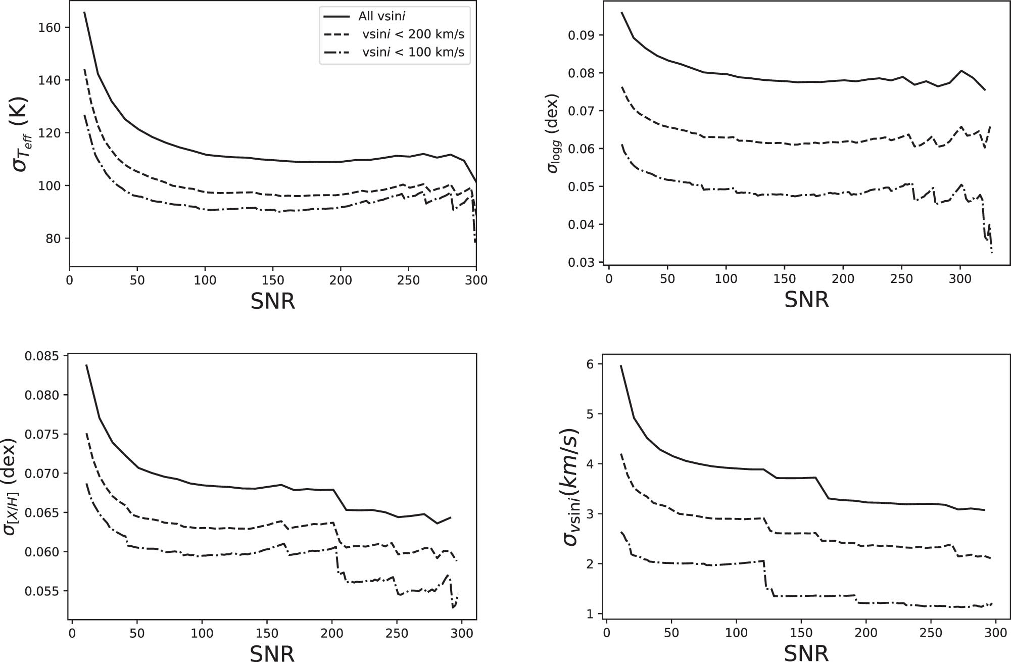
Average error bars for the observation predicted stellar parameters as a function of the SNR and for different ranges of stellar rotation.

6 Extrapolating to other spectral-types

In order to verify how universal the results are, we checked that the optimization of the code is not dependent on wavelength and/or spectral-type, we also tested the procedure on FGK stars. To do that, we have calculated a TDB specific for FGK stars using the parameters displayed in Table 4. The wavelength range was selected to coincide with the one of Paletou et al. (2015a). This range is sensitive to all the concerned stellar parameters.

A database of 50,000 random synthetic spectra with known stellar labels is used in the training. About 20,000 test data, with and without noise, were calculated in the same range of Table 4 to be used for verification. The optimal NNs that were introduced in Section 5 were used again, as a proof of concept, for the FGK TDB. The results are displayed in Table 5 for training, validation, and tests.

Because of the low rotational velocities for FGK stars ( v e sin i < 100 km s − 1 ), the results are more accurate. That is not surprising because v e sin i drastically affects the shape of the lines as in A stars. The derived errors on the stellar parameters are found to be 82 K, 0.07 dex, 0.90  km s − 1 , and 0.06 dex for T eff , log g , v e sin i , and [M/H], respectively (Table 5). These results are very promising, but we should be aware of the complications that would arise when using real observations, especially in the case of the cool M stars. These stars have been analysed in the context of exoplanet search (Shan et al. 2021, Passegger et al. 2020) and show complications in their spectra mainly related to the continuum normalization. Adapting the data preparation and the CNN will be inevitable in order to take into account these effects. These results also show that when deriving the stellar parameters for specific spectral-types, the wavelength region should be selected according to these spectral lines/bands most sensitive to the variations of the parameters one seeks.

7 Discussion and conclusion

The purpose of this work is not only to find the best tool for the accurate prediction of parameters but also to show the steps that should be taken in order to reach the optimal selection of the CNN parameters. Often scientists use DL as a black box without explaining the choice of the parameters and/or architecture. In this manuscript, we have explained the reason for selecting specific hyperparameters while emphasizing the pedagogical approach. To have a more effective tool, one should change the architecture of the model. The architecture of the model depends on the type and range of the input. In this work, we have fixed the architecture and iterated on the hyperparameters only. Sections 5.1–5.4 show that for each stellar parameter, the setup of the network should be changed. This means that for a specific network and a specific stellar parameter, a study should be made to find the optimal configuration of hyperparameters. This is due to the contribution of the specific stellar parameter on the shape of the input spectrum. Using the PCA decomposition, we have reduced the size of the input parameters to only 50 points per spectrum while keeping more than 99.5% of the information. This is recommended in case of large databases and wide wavelength range and could avoid the use of extra pooling layers in the network. This projection technique is not only applicable for AFGK stars but can also be used for cooler stars. Furthermore, (Houdebine et al. 2016, Paletou et al. 2015b), Sarro et al. (2018) have applied a projection pursuit regression model based on the independent component analysis compression coefficients to derive T eff , log g , and [M/H] of M-type stars.

Although the CNN architecture was not optimized, we were able, using a strategy of finding the best hyperparameters, to reach a level of accuracy that is comparable to other adopted techniques. In fact, we found for A stars, an average accuracy of 0.08 dex for log g , 0.07 dex for [M/H], 3.90 km s − 1 for v e sin i , and 127 K for T eff . In the case of stars with v e sin i less than 100 km s − 1 , we found the accuracy to be 90 K, 0.06 dex, 0.06 dex, and 2.0 km s − 1 , for T eff , log g , [M/H] and v e sin i , respectively. These accuracy values are signal to noise dependant and reduce as long as the signal to noise increases. Extrapolating the technique to FGK stars also shows that the same network could be applied to different spectral-types and different wavelength ranges.

The technique that we followed in this article could be transferable to any classification problem that involves neural network. In the future, we plan to develop a strategy to find the best CNN architecture depending on the input data and the type of the predicted parameters. Once the architecture and the configuration of the parameters are settled, we will be testing the procedure on observational spectra as we did in the studies of Paletou et al. (2015a), Paletou et al. (2015b), Gebran et al. (2016), and Kassounian et al. (2019). Using only observational data or a combination of synthetic spectra and real observations with well-known parameters will allow us to constrain the derived stellar labels while minimizing the critical synthetic gap (Fabbro et al. 2018). One more criterion that should be taken into account is when applying this technique to real observations, thorough data preparation work should be done to take into account the characteristics of each spectral-type (e.g. continuum normalization in M and giant stars, and low number of lines in hot stars).

References

Almeida I, Duarte R, Nemmen R. 2021. Deep learning model for multiwavelength emission from low-luminosity active galactic nuclei. arXiv e-prints. page arXiv: 2102.05809.Search in Google Scholar
Anthony M, Bartlett PL. 1999. Neural Network Learning: Theoretical Foundations. Cambridge: Cambridge University Press.10.1017/CBO9780511624216Search in Google Scholar
Aydi E, Gebran M, Monier R, Royer F, Lobel A, Blomme R. 2014. Automated procedure to derive fundamental parameters of B and A stars: Application to the young cluster NGC 3293. In: Ballet J, Martins F, Bournaud F, Monier R, Reylé C, editors, SF2A-2014: Proceedings of the Annual meeting of the French Society of Astronomy and Astrophysics, p. 451–455.Search in Google Scholar
Bai Y, Liu J, Bai Z, Wang S, Fan D. 2019. Machine-learning regression of stellar effective temperatures in the second gaia data release. AJ, 158(2):93.10.3847/1538-3881/ab3048Search in Google Scholar
Bailer-Jones CAL. 1997. Neural network classification of stellar spectra. PASP. 109:932.10.1007/978-1-4612-1968-2_42Search in Google Scholar
Baron D. 2019. Machine Learning in Astronomy: a practical overview. arXiv e-prints, page arXiv: 1904.07248.Search in Google Scholar
Bengio Y. 2012. Practical recommendations for gradient-based training of deep architectures. In Neural networks: tricks of the trade. Berlin, Heidelberg: Springer.10.1007/978-3-642-35289-8_26Search in Google Scholar
Bickley RW, Bottrell C, Hani MH, Ellison SL, Teimoorinia H, Yi KM, et al. 2021. Convolutional neural network identification of galaxy post-mergers in UNIONS using IllustrisTNG. MNRAS. 504:372–92.10.1093/mnras/stab806Search in Google Scholar
Castelli F, Kurucz RL. 2003. New grids of ATLAS9 model atmospheres. In Piskunov N, Weiss WW, Gray DF, editors. Modelling of Stellar Atmospheres. vol. 210, p. A20.Search in Google Scholar
Chen BH, Goto T, Kim SJ, Wang TW, Santos DJD, Ho SCC, et al. 2021. An active galactic nucleus recognition model based on deep neural network. MNRAS, 501(3):3951–3961.10.1093/mnras/staa3865Search in Google Scholar
Choi D, Shallue CJ, Nado Z, Lee J, Maddison CJ, Dahl GE. 2020. On empirical comparisons of optimizers for deep learning. arXiv preprint arXiv:1910.05446.Search in Google Scholar
Cropper M, Katz D, Sartoretti P, Panuzzo P, Seabroke G, Smith M, et al. 2014. Gaia radial velocity spectrometer performance. In EAS Publications Series. vol. 67–68 p. 69–73.10.1051/eas/1567011Search in Google Scholar
Curran SJ, Moss JP, Perrott YC. 2021. QSO photometric redshifts using machine learning and neural networks. MNRAS. 503:2639–2650.10.1093/mnras/stab485Search in Google Scholar
Dafonte C, Fustes D, Manteiga M, Garabato D, Álvarez MA, Ulla A, et al. 2016. On the estimation of stellar parameters with uncertainty prediction from generative artificial neural networks: application to Gaia RVS simulated spectra. A&A. 594:A68.10.1051/0004-6361/201527045Search in Google Scholar
Fabbro S, Venn KA, O’Briain T, Bialek S, Kielty CL, Jahandar F, et al. 2018. An application of deep learning in the analysis of stellar spectra. MNRAS. 475(3):2978–2993.10.1093/mnras/stx3298Search in Google Scholar
Gafeira R, Orozco Suárez D, Milić I, Quintero Noda C, Ruiz Cobo B, Uitenbroek H. 2021. Machine learning initialization to accelerate Stokes profile inversions. A&A. 651:A31.10.1051/0004-6361/201936910Search in Google Scholar
Gan FK, Bekki K, Hashemizadeh H. 2021. SeeingGAN: Galactic Image Deblurring with Deep Learning for Better Morphological Classification of Galaxies. arXiv e-prints, page arXiv:2103.09711.Search in Google Scholar
Garraffo C, Protopapas P, Drake JJ, Becker I, Cargile P. 2021. StelNet: Hierarchical Neural Network for Automatic Inference in Stellar Characterization. arXiv e-prints, page arXiv:2106.07655.10.3847/1538-3881/ac0ef0Search in Google Scholar
Gebran M, Farah W, Paletou F, Monier R, Watson V. 2016. A new method for the inversion of atmospheric parameters of A/Am stars. A&A. 589:A83.10.1051/0004-6361/201528052Search in Google Scholar
Gebran M, Monier R, Royer F, Lobel A, Blomme R. 2014. Microturbulence in A/F Am/Fm stars. In Mathys G, Griffin ER, Kochukhov O, Monier R, Wahlgren GM, editors. Putting A Stars into Context: Evolution, Environment, and Related Stars, Proceedings of the International Conference. 2013 Jun 3–7; Moscow, Russia. p. 193–198.Search in Google Scholar
Gill S, Maxted PFL, Smalley B. 2018. The atmospheric parameters of FGK stars using wavelet analysis of CORALIE spectra. A&A. 612:A111.10.1051/0004-6361/201731954Search in Google Scholar
Glorot X, Bengio Y. 2010. Understanding the difficulty of training deep feedforward neural networks. In Teh YW, Titterington M, editors. Proceedings of the 13th International Conference on Artifficial Intelligence and Statistics. 2010 May 13–15; Sardinia, Italy. JMLR, 2010. p. 249–256.Search in Google Scholar
Glorot X, Bordes A, Bengio Y. 2011. Deep sparse rectifier neural networks. In Gordon G, Dunson D, DudÃÂŋk M, editors. Proceedings of the Fourteenth International Conference on Artificial Intelligence and Statistics, volume 15 of Proceedings of Machine Learning Research. p. 315–323. FL, USA: Fort Lauderdale, JMLR Workshop and Conference Proceedings.Search in Google Scholar
González-Marcos A, Sarro LM, Ordieres-Meré J, Bello-García A. 2017. Evaluation of data compression techniques for the inference of stellar atmospheric parameters from high-resolution spectra. MNRAS. 465(4):4556–4571.10.1093/mnras/stw3031Search in Google Scholar
Goodfellow I, Bengio Y, Courville A. 2016. Deep Learning. MIT Press. http://www.deeplearningbook.org.Search in Google Scholar
Guiglion G, Matijevič G, Queiroz ABA, Valentini M, Steinmetz M, Chiappini C, et al. 2020. The RAdial Velocity Experiment (RAVE): Parameterisation of RAVE spectra based on convolutional neural networks. A&A. 644:A168.10.1051/0004-6361/202038271Search in Google Scholar
He K, Zhang X, Ren S, Sun J. 2015. Delving deep into rectifiers: Surpassing human-level performance on imagenet classification. In 2015 IEEE International Conference on Computer Vision (ICCV). p. 1026–1034. 10.1109/ICCV.2015.123.Search in Google Scholar
Houdebine ER, Mullan DJ, Paletou F, Gebran M. 2016. Rotation-activity correlations in K and M Dwarfs. I. Stellar Parameters and Compilations of v sin I and P/sin I for a Large Sample of Late-K and M Dwarfs. ApJ. 822(2):97.10.3847/0004-637X/822/2/97Search in Google Scholar
Hubeny I, Lanz T. 1992. Accelerated complete-linearization method for calculating NLTE model stellar atmospheres. A&A. 262(2):501–514.Search in Google Scholar
Jaitly N, Hinton E. 2013. Vocal tract length perturbation (VTLP) improves speech recognition. In Proceedings on ICML Workshop on Deep Learning for Audio, Speech and Language. vol. 117: p. 21.Search in Google Scholar
Kassounian S, Gebran M, Paletou F, Watson V. 2019. Sliced Inverse Regression: application to fundamental stellar parameters. Open Astron. 28(1):68–84.10.1515/astro-2019-0006Search in Google Scholar
Keskar NS, Mudigere D, Nocedal J, Smelyanskiy M, Tang PTP. 2016. On large-batch training for deep learning: Generalization gap and sharp minima. cite arxiv:1609.04836 Comment: Accepted as a conference paper at ICLR 2017.Search in Google Scholar
Kurucz RL. 1992. Atomic and molecular data for opacity calculations. RMXAA. 23:45.Search in Google Scholar
Landa V, Reuveni Y. 2021. Low dimensional convolutional neural network for solar flares GOES time series classification. arXiv e-prints, page arXiv: 2101.12550.Search in Google Scholar
Lecun Y, Bottou L, Bengio Y, Haffner P. 1998. Gradient-based learning applied to document recognition. Proc IEEE. 86(11):2278–2324.10.1109/5.726791Search in Google Scholar
LeCun Y. 1989. Generalization and network design strategies. Connectionism Perspect. 19:143–155.Search in Google Scholar
Li X-R, Pan R-Y, Duan F-Q. 2017. Parameterizing stellar spectra using deep neural networks. Res Astronom Astrophys. 17(4):36.10.1088/1674-4527/17/4/36Search in Google Scholar
Maas AL. 2013. Rectifier nonlinearities improve neural network acoustic models. In Proc ICML. Vol. 30, No. 1, p. 3.Search in Google Scholar
Neyshabur B, Bhojanapalli S, Mcallester D, Srebro N. 2017. Exploring generalization in deep learning. In Guyon I, Luxburg UV, Bengio S, Wallach H, Fergus R, Vishwanathan S, et al. editors. Advances in Neural Information Processing Systems. vol 30, p. 5947–5956. Curran Associates, Inc.Search in Google Scholar
Ofman L, Averbuch A, Shliselberg A, Benaun I, Segev D, Rissman A. 2022. Automated identification of transiting exoplanet candidates in NASA Transiting Exoplanets Survey Satellite (TESS) data with machine learning methods. New Astron. 91:101693.10.1016/j.newast.2021.101693Search in Google Scholar
Paletou F, Böhm T, Watson V, Trouilhet JF. 2015a. Inversion of stellar fundamental parameters from ESPaDOnS and Narval high-resolution spectra. A&A. 573:A67.10.1051/0004-6361/201424741Search in Google Scholar
Paletou F, Gebran M, Houdebine ER, Watson V. 2015b. Principal component analysis-based inversion of effective temperatures for late-type stars. A&A. 580:A78.10.1051/0004-6361/201526828Search in Google Scholar
Parks D, Prochaska JX, Dong S, Cai Z. 2018. Deep learning of quasar spectra to discover and characterize damped Lyα systems. MNRAS. 476(1):1151–1168.10.1093/mnras/sty196Search in Google Scholar
Passegger VM, Bello-García A, Ordieres-Meré J, Antoniadis-Karnavas A, Marfil E, Duque-Arribas C, et al. 2021. Metallicities in M dwarfs: Investigating different determination techniques. arXiv e-prints, page arXiv: 2111. 14950.10.1051/0004-6361/202141920Search in Google Scholar
Passegger VM, Bello-García A, Ordieres-Meré J, Caballero JA, Schweitzer A, González-Marcos A, et al. 2020. The CARMENES search for exoplanets around M dwarfs. A deep learning approach to determine fundamental parameters of target stars. A&A. 642:A22.10.1051/0004-6361/202038787Search in Google Scholar
Portillo SKN, Parejko JK, Vergara JR, Connolly AJ. 2020. Dimensionality reduction of SDSS spectra with variational autoencoders. AJ. 160(1):45.10.3847/1538-3881/ab9644Search in Google Scholar
Ramírez Vélez JC, Yáñez Márquez C, Córdova Barbosa JP. 2018. Using machine learning algorithms to measure stellar magnetic fields. A&A. 619:A22.10.1051/0004-6361/201833016Search in Google Scholar
Rhea C, Rousseau-Nepton L. 2021. Application of machine learning to optical spectra – kinematic constraints. In American Astronomical Society Meeting Abstracts. volume 53 of American Astronomical Society Meeting Abstracts. 208.01.Search in Google Scholar
Rhea C, Rousseau-Nepton L, Prunet S, Hlavacek-Larrondo J, Fabbro S. 2020. A machine-learning approach to integral field unit spectroscopy observations. I. H ii region kinematics. ApJ. 901(2):152.10.3847/1538-4357/abb0e3Search in Google Scholar
Rosasco L, Vito ED, Caponnetto A, Piana M, Verri A. 2004. Are loss functions all the same? Neural Comput. 16(5):1063–1076.10.1162/089976604773135104Search in Google Scholar PubMed
Ruder S. 2016. An overview of gradient descent optimization algorithms. CoRR. abs/1609.04747.Search in Google Scholar
Sarro LM, Ordieres-Meré J, Bello-García A, González-Marcos A, Solano E. 2018. Estimates of the atmospheric parameters of M-type stars: a machine-learning perspective. MNRAS. 476(1):1120–1139.10.1093/mnras/sty165Search in Google Scholar
Shan Y, Reiners A, Fabbian D, Marfil E, Montes D, Tabernero HM, et al. 2021. The CARMENES search for exoplanets around M dwarfs. Not-so-fine hyperfine-split vanadium lines in cool star spectra. A&A. 654:A118.10.1051/0004-6361/202141530Search in Google Scholar
Sharma K, Kembhavi A, Kembhavi A, Sivarani T, Abraham S, Vaghmare K. 2020. Application of convolutional neural networks for stellar spectral classification. MNRAS. 491(2):2280–2300.10.1093/mnras/stz3100Search in Google Scholar
Shorten C, Khoshgoftaar T. 2019. A survey on image data augmentation for deep learning. J Big Data. 6:1–48.10.1186/s40537-019-0197-0Search in Google Scholar
Smalley B. 2004. Observations of convection in A-type stars. In Zverko J, Ziznovsky J, Adelman SJ, Weiss WW, editors. Proceedings of the International Astronomical Union 2004 (IAUS224), The A-Star Puzzle. p. 131–138. Cambridge, UK: Cambridge University Press.10.1017/S1743921304004478Search in Google Scholar
Srivastava N, Hinton G, Krizhevsky A, Sutskever I, Salakhutdinov R. 2014. Dropout: a simple way to prevent neural networks from overfitting. J Mach Learn Res. 15(1):1929–1958.Search in Google Scholar
Wang R, Luo AL, Chen J-J, Hou W, Zhang S, Zhao Y-H, LAMOST MRS collaboration, et al. 2020. SPCANet: stellar parameters and chemical abundances network for LAMOST-II medium resolution survey. ApJ. 891(1):23.10.3847/1538-4357/ab6deaSearch in Google Scholar
Wang S-C. 2003. Artificial neural network. pp. 81–100. US, Boston, MA: Springer.10.1007/978-1-4615-0377-4_5Search in Google Scholar
Yim J, Ju J, Jung H, Kim J. 2015. Image classification using convolutional neural networks with multi-stage feature. In Kim J-H, Yang W, Jo J, Sincak P, Myung H, editors. Robot Intelligence Technology and Applications 3. Cham: Springer International Publishing, p. 587–594.10.1007/978-3-319-16841-8_52Search in Google Scholar
Zhang B, Liu C, Deng L-C. 2020. Deriving the Stellar Labels of LAMOST Spectra with the Stellar LAbel Machine (SLAM). ApJS. 246(1):9.10.3847/1538-4365/ab55efSearch in Google Scholar
Zhang C, Bengio S, Hardt M, Recht B, Vinyals O. 2016. Understanding deep learning requires rethinking generalization. In 5th International Conference on Learning Representations, ICLR 2017 - Conference Track Proceedings. arXiv:1611.03530.10.1145/3446776Search in Google Scholar
Zhou Y-T, Chellappa R. 1988. Computation of optical flow using a neural network. In ICNN. p. 71–78.10.1109/ICNN.1988.23914Search in Google Scholar
Zhu X, Vondrick C, Fowlkes CC, Ramanan D. 2016. Do we need more training data? Int J Comput Vision. 119(1):76–92.10.1007/s11263-015-0812-2Search in Google Scholar
Zou D, Cao Y, Zhou D, Gu Q. 2019. Gradient descent optimizes over-parameterized deep relu networks. Mach Learn. 109:467–492.10.1007/s10994-019-05839-6Search in Google Scholar
© 2022 Marwan Gebran et al., published by De Gruyter
This work is licensed under the Creative Commons Attribution 4.0 International License.
Articles in the same Issue
- Research Articles