Investigation of the mechanism of a solar flare by means of MHD simulations above the active region in real scale of time: The choice of parameters and the appearance of a flare situation

1 Introduction: the need for magnetohydrodynamic (MHD) simulations above the active region (AR) in the real scale of time to study the solar flare mechanism

Solar flares are the most powerful manifestations of solar activity, during which energy of 1 0 32 erg is released in a few tens of minutes. Since flares occur above ARs with a large magnetic field (the value of the field in the AR on the solar surface reaches several thousand G), there is now no doubt that magnetic energy is released during flares. The primordial energy release from the flare occurs high in the solar atmosphere (in the lower corona) at altitudes of 15,000–70,000 km, which is ∼1/40–1/10 of the solar radius. First of all, this has been proven by direct measurements of the thermal X-ray emission of flares on the limb (Lin et al. 2003). Evidence of the appearance of a flare in the corona is also the invariability of the magnetic field on the solar surface (Podgorny et al. 2015), and the analysis of temperature changes in time in the corona at the flare site according to observations of ultraviolet radiation of highly ionized iron ions (Podgorny and Podgorny 2018).

The main flare process high in the corona can be explained by the mechanism of Syrovatskii (1966): the accumulation of magnetic energy in the field of a current sheet, which is formed in the vicinity of an X-type singular line of magnetic field. As a result of quasi-stationary evolution, the current sheet transfers into an unstable state (Podgorny and Podgorny 2012). Instability causes a flare release of energy with all the observed manifestations of a flare, which are explained by the electrodynamic model of a flare proposed by I. M. Podgorny (Podgorny et al. 2010). The model was developed based on the results of observations and numerical MHD simulation and uses analogies with the electrodynamic substorm model proposed earlier by the author on the basis of Intercosmos-Bulgaria-1300 satellite data (Podgorny et al. 1988). The hard X-ray beam radiation on the surface of the sun during a flare is explained by the deceleration in the lower dense layers of the solar atmosphere of electron fluxes accelerated in field aligned currents caused by the Hall electric field in the current sheet. Studies have once again confirmed that the only mechanism that can explain the slow accumulation of magnetic energy in the solar corona in a stable configuration, and then its rapid release during a flare when the configuration transition to an unstable state, is the mechanism of the release of energy accumulated in the magnetic field of the current sheet.

Since the configuration of the magnetic field in the corona cannot be obtained from observations, in order to study the physical mechanism of the flare, as well as improve the prognosis of flares, it is necessary to carry out MHD simulation in the corona above the AR, in which all conditions are taken from observations. The results of recent studies lead to the conclusion that in order to study the mechanism of a solar flare, the calculation should begin several days before the appearance of flares, when the magnetic energy for the flare has not yet accumulated in the corona. When setting the problem, no assumptions about the flare mechanism were made at setting of the problem (Podgorny and Podgorny 2008), the purpose of the simulation was to determine the mechanism of the solar flare. For setting the boundary conditions, we used the magnetic field distribution observed in the photosphere; the other conditions were approximated by the free exit conditions.

The problem of studying the mechanism of a solar flare by MHD simulation of a flare situation in the corona above a real AR has not been completely solved at present. The problem is so complex that it cannot be completely solved using the already developed numerical methods, even using the most powerful computing clusters, such as the NASA Ames Research Center, with parallel computing on modern graphics cards (GPU). It is necessary to develop and optimize mathematical methods and to program the most optimal algorithm for parallel calculations specifically for our problem.

In order to speed up the calculation, a finite-difference scheme was specially developed, which had to remain stable for the largest possible time step (Podgorny and Podgorny 2004, 2008). The scheme was realized in the PERESVET program. The scheme is upwind, absolutely implicit, and conservative with respect to the magnetic flux, it is solved by the iteration method. Despite the use of specially developed methods, it was possible to carry out MHD simulations in the corona on a usual computer only on a greatly reduced (by a factor of 1 0 4 ) time scale (Podgorny and Podgorny 2013a, b, Podgorny et al. 2017, 2018). At MHD simulations on a greatly reduced time scale, instability arose at the photospheric boundary, caused by an unnaturally rapid change in the magnetic field; however, thanks to the application of the developed methods, it did not propagate into the calculated region of the corona and did not increase to infinity. In order to get rid of this instability, as well as to obtain the correct development of processes in time, it is necessary to carry out MHD simulations in real scale of time.

Since it is impossible to carry out MHD simulation in the corona in the real scale of time on a conventional computer for the foreseeable calculation time, it is necessary to carry out parallel computations using the CUDA technology (Borisenko et al. 2020a, b). Compute unified device architecture (CUDA) is the system of programming of parallel computations on graphic cards (GPU). At MHD simulations in the real scale of time, instabilities do not appear near the photospheric boundary caused by an unnaturally fast change in the magnetic field at the boundary. However, both near the photospheric boundary and near the non-photospheric boundary, instabilities arise, which have time to develop during a sufficiently long period of calculation time. To stabilize these instabilities, special methods have been developed and applied.

The physical and methodological results obtained make it possible to develop a plan for upgrading the methods of MHD simulation in the solar corona, including methods for stabilizing instabilities, which should make it possible to more accurately study the flare situation above the AR.

2 Computational domain and improving of methods for the MHD simulation

MHD simulation is performed in computational domain in corona above the AR 1 × 0.3 × 1 ( 0 < x < 1 , 0 < y < 0.3 , 0 < z < 1 ) (dimensionless unit of length is chosen as L 0 = 4 × 1 0 10 cm ). Y axis is directed from the Sun perpendicular to the photosphere, the y = 0 ( X , Z ) plane is located on the photosphere, the X axis is directed from East to West, the Z axis is directed from North to South. MHD simulation is performed above AR 10365 during 2.5 days from the moment May 24, 2003 at 20:48. The magnetic field measured on the photosphere by SOHO MDI (http://soi.stanford.edu/magnetic/index5.html) is used for setting boundary conditions.

The time of calculation of evolution of the field and plasma in the solar corona above the AR is determined by:

1. The size of the time step (at which the scheme remains stable).

2. The number of iterations.

3. The time of calculation of one iteration.

These values depend on:

1. Mathematical method: The type of difference scheme (within a given type of scheme, which is absolutely implicit and conservative with respect to the magnetic flux) and the parameters of the difference scheme, first of all, ordinary and artificial magnetic viscosity, which is used mainly near the boundary (where difficulties always arise with the correct setting of all boundary conditions).

2. The computation speed of a given processor, for us, is, first of all, the computation speed of graphics card (GPU) threads, which perform parallel computations.

3. Algorithm for parallelizing computations, in particular, the location and transfer of arrays on the graphics card, which are, in essence, copies of the arrays of distributions of all quantities in the computational domain contained in the main memory of the computer.

Parallelization of computations was carried out using CUDA technology on modern graphics cards (GPU). The modern software (Fortran PGI) was used. The methods of optimizing the parallelization of calculations were developed including minimization of data exchange between the memory of GPU and the memory of central processor.

For optimization of the algorithm parallelization calculation, more than 20 modernizations of the code were performed, as the result of which the speed of calculation increases 7.5 times and became 120 times faster than the calculation speed of a non-parallel program, in which the same difference scheme is realized. After the performed optimization, the computation time for one iteration on the used grid of the difference scheme 135 × 41 × 135 was 0.02 s.

3 Choice of parameters of MHD equations. Stabilization of instabilities arising near the boundary

The time step τ should not significantly exceed the time from Courant’s condition τ K : τ < τ K = h / ( V MV + V MA ) . Here h is the spatial step, V MV is the maximum of the velocity absolute value, and V MA is the maximum value of the absolute values of the magnetosonic and Alfven velocities. Calculations have shown that the time step τ should be less than τ K , despite the fact that an absolutely implicit scheme is used (apparently due to the fact that the system of equations with cross terms and the iteration method are used).

It was hoped that simulations in the real scale of time would eliminate the instability near the photospheric boundary caused by an unnaturally rapid change in the magnetic field in the photosphere when simulated on a greatly reduced time scale. However, as experience has shown, due to the difficulties in matching the solution in the computational domain with the values specified at the boundary, a calculation in the real scale time can lead to the development of a strong instability that has time to develop during a long time interval, both near the photosphere and non-photospheric boundaries. The strongest instabilities arise at low viscosities (magnetic and ordinary).

The problem of stabilization of instabilities arising at the boundaries of the computational domain was almost completely solved (Podgorny et al. 2020), for which artificial limitation of the rate of plasma inflow into the computational domain through the non-photospheric boundary, specifying weakly varying magnetic field components parallel to the boundary at the non-photospheric boundary (the perpendicular field components when using a finite-difference scheme conservative with respect to the magnetic flux are always specified from the condition [ div B ] = 0 ), the setting of artificial viscosity near the non-photospheric boundary, and other stabilization methods were used.

The viscosities were set in accordance with the principle of limited simulation (Podgorny 1978), according to which much larger or much smaller units, dimensionless parameters remain much larger or smaller than units when simulated without their exact preservation.

The principle of limited simulation was applied on the basis that the magnetic viscosity in the calculated region of the corona corresponds to the magnetic Reynolds number Rm = 1 0 16 (corresponds to a velocity of 0.65 × 1 0 10 cm / s , equal to the Alfven velocity V A = 4 π ρ for a corona density of 1 0 8 cm − 3 and a typical field in the corona region of 300 G), the usual viscosity corresponds to the Reynolds number Re = 1 0 4 and the Reynolds number across the magnetic field Re B = 1 0 20 . When choosing the dimensionless parameters, it was taken into account that the selected dimensionless viscosity (inverse to the Reynolds number ν = Re − 1 ) should not be less than the dimensionless grid viscosity ν grid = h V DimLess by more than 2–3 orders of magnitude ( h is the dimensionless grid step in units equal to the size of the region L 0 = 4 × 1 0 10 cm , for the selected grid h = 0.5 × 1 0 − 2 ; V DimLess is the dimensionless plasma velocity in units equal to the typical Alfven velocity V A = 0.65 × 1 0 10 cm / s , in the calculations the velocities V DimLess = 1 0 − 6 ÷ 1 0 − 3 appear). Of course, it would be better if the grid viscosity was always less than the specified viscosity (in this case, the thickness of the current sheet will be determined by the specified viscosity, not the grid), but this cannot be done if we want a sufficiently good fulfill of freezing-in condition at the initial stage of the formation of the current sheet, when the plasma velocity is still low ( V DimLess = 1 0 − 6 ).

For AR 10365, two calculations were carried out for two sets of parameters corresponding to relatively high and low viscosities within 3 days (Figure 1). In both calculations near the non-photospheric boundary, to stabilize the numerical instability, sufficiently large artificial viscosities were taken, their dimensionless values (inverse to the Reynolds numbers) are ν Art = ν mArt = 1 0 − 1 ÷ 1 0 − 2 .

Figure 1

Viscosity and artificial viscosity for two calculation variants.

In the first variant, the viscosities were taken equal to ν m = 0.3 × 1 0 − 5 ( R m = 3 × 1 0 5 ); ν = 1 0 − 4 ( Re = 1 0 4 ), the artificial viscosity near the photospheric boundary was taken relatively high ν Art Ph , ν m Art Ph = 0.3 × 1 0 − 2 . With these parameters, due to the suppression of the perturbation propagating from the photosphere by the artificial viscosity, a sufficiently intense accumulation of the flare energy does not occur in the region; therefore, a calculation with the second set of parameters with significantly lower viscosities was required. The calculation results with these parameters are given in Podgorny et al. (2020).

In the second variant of the calculation, a set of parameters was selected ν m = 1 0 − 9 ( Rm = 1 0 9 ); ν = 1 0 − 7 ( Re = 1 0 7 ); ν Art Ph , ν m Art Ph = 1 0 − 4 , the simulation results with these parameters are presented in the next chapter.

If instabilities did not arise at the boundary, then, proceeding only from the need to obtain a stable solution inside the region, it is possible to make the following estimate of the computation time of one day of evolution in the solar corona above the AR. The time step from the Courant condition τ K = h / ( V MV + V MA ) in the calculations is τ K = 1 0 − 8 ÷ 1 0 − 7 days. To estimate the computation time with a step τ K : the computation time of one iteration on graphics cards using the CUDA technology is 2 × 1 0 − 2 s , for five iterations the computation time of one step is 0.1 s, so that ( day ∼ 1 0 5 s ) the computation time of 1 day of evolution in the solar corona is 10 ÷ 100 days. At low viscosities, strong disturbances arise in some places of the computational domain (first of all, in places of accumulation of energy for flares). In the calculations according to the chosen difference scheme, such perturbations did not cause numerical instability within the region, as a result of which the continuation of the calculation becomes impossible. However, these disturbances are propagating towards the boundary. The perturbations are so strong that, despite setting a large artificial viscosity near the boundary, they cause numerical instability due to the inconsistency of the numerical solution with the boundary conditions, the elimination of which is one of the main problems of numerical methods for solving partial differential equations. For this set of parameters, the use of only the introduced methods is not enough; to stabilize the instabilities, it is also necessary to decrease the step (less than 1 0 − 8 days) and increase the number of iterations (in the calculations, their number reached 60 and more). As a result, the calculation time is greatly increased, reaching several months.

4 MHD simulation results. Flare M1.4 27.05.2003 at 2:43

MHD simulation above AR 10365 showed the appearance of singular lines in which a diverging magnetic field is superimposed on the configuration of the X-type magnetic field (Figure 2). For our purposes, it is more convenient to represent the X-type field configuration (Figure 2a) in the coordinate system rotated by 4 5 ∘ (Figure 2b). In this system, the X and Y coordinates are directed along the eigenvectors of the matrix ∇ B represented in the coordinate system with the Z axis directed along the magnetic field vector at the point of maximum current density. The matrix with field components in the X Y plane is diagonal for the matrix ∇ B (Figure 2c), since for the Z coordinates directed along the singular line, the components of the third row of the matrix ∇ B ∂ B z / ∂ x , ∂ B z / ∂ y and its third column ∂ B x / ∂ z , ∂ B y / ∂ z are equal to zero (actually, in the calculation on singular lines passing through the position of the maximum of the current density, these values are close to zero). The eigenvalues of the matrix ∇ B determine the configuration of the field in the vicinity of the singular line of the magnetic field. First of all, this is the configuration in the X Y plane, perpendicular to the singular line, which is called in Podgorny et al. (2017) the plane of the configuration of the current sheet, since MHD simulation shows that in this plane, the current sheet is most pronounced.

Figure 2

Superposition of X-type magnetic field and diverging magnetic field. (a) plane X-type configuration in usual coordinate system and (b) in the coordinate system rotated by 45°, in which it is convenient to consider the superposition of magnetic fields. (c) matrix ∇B, its representation in chosen coordinate system through eigenvalues, expression for magnetic lines of superimposed fields. (d) illustration of fields superposition

When the X-type field and the diverging field are superimposed (Figure 2d), the magnetic lines of the resulting field have the form y = C x α , where α = λ 2 / λ 1 , λ 1 , and λ 2 are the eigenvalues of the matrix ∇ B (Podgorny 1989). If the X-type field dominates, then the magnetic lines have the form of hyperbolas ( α < 0 , λ 1 and λ 2 have different signs). If the diverging field dominates, then the magnetic lines have the shape of parabolas ( α > 0 , λ 1 and λ 2 of the same sign). j × B magnetic forces in X-type configuration collect disturbances into current sheet (Figure 3a) and for diverging magnetic field cause rotation of plasma around the singular line (Figure 3b).

Figure 3

j × B forces for X-type configuration (a) and diverging magnetic field (b).

Examples of magnetic field configurations with plasma flow obtained as a result of MHD simulation are presented in Figure 4. The diverging magnetic field can be large, it can dominate the X-type field, fundamentally distorting its configuration. However, even in this case, the presence of the X-type configuration leads to the accumulation of perturbations with the formation of a current sheet, in the magnetic field of which the flare energy is accumulated. In this case, even with a dominant diverging magnetic field, a sufficiently powerful current sheet may appear (Figure 4, J Max 5, lower left corner; and even more powerful current sheet in Figure 7, J Max 4), which can lead to the appearance of not only a weak flare but also a flare of medium power.

Figure 4

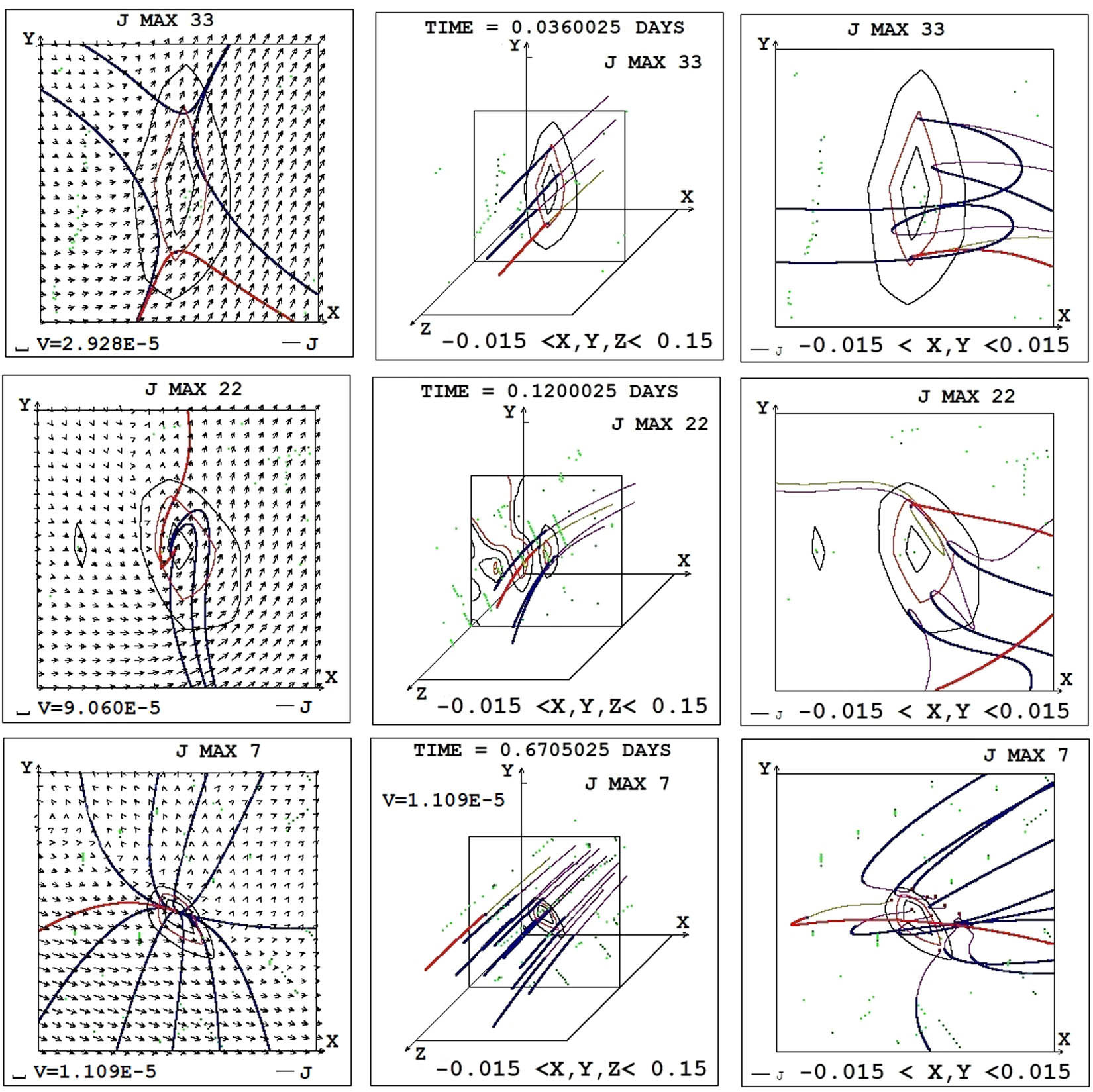
Examples of superposition of X-type and diverging magnetic field near current density maxima situated on singular lines obtained from MHD simulation. Magnetic field configurations and plasma flow in the plane of configuration which is perpendicular to the vector of magnetic field in the point of current density maximum. Plane magnetic field configuration is represented by lines tangent to the projections of the magnetic field vectors on the plane of configuration. The scale of the velocity vector is shown in dimensionless units (the unit is typical Alfven velocity equal to V A = 0.65 × 1 0 10 cm / s ). Constant current density lines are presented as thin lines. The linear size of region is 0.03 (12 mM).

Most often, the three-dimensional configuration of the magnetic field in the vicinity of the singular line is complex (examples are shown in Figure 5), from this configuration it is impossible to determine that the line is singular. Therefore, a system for finding points through which singular line pass is required. To study the field configuration in the vicinity of singular lines, we used a specially developed graphical system for searching for flare positions from the results of MHD simulation (Podgorny and Podgorny 2013a,b, Podgorny et al. 2017). The graphical system for searching is based on the fact that the absolute value of the current density is maximal in the middle of the current sheet. The positions of all local maxima of the current density are sought. In the vicinity of the point of maximum current density, which lie on an X-type singular line, the configuration of the magnetic field is investigated. The analysis of the magnetic field configuration is carried out primarily in the so-called configuration plane, i.e., in the plane perpendicular to the magnetic field vector. This vector is taken at the point of maximum current density. In this plane, the configuration of the magnetic field of the current sheet is most pronounced.

Figure 5

Field configurations near singular lines in the region with a linear size of 0.03 dimensionless units (12 mM) in the centers of which the maxima of the current density are located. The Z axis is directed along the magnetic field vector taken at the point of maximum current density. The plane ( X , Y ) perpendicular to the magnetic field vector is the plane of the configuration in which the current sheet is best expressed. Left column: Plane magnetic field configurations and plasma flows as on panels of Figure 4. Middle column: 3D configurations of the magnetic field near the point of maximum current density. Right column: Projections of magnetic lines onto the plane of the configuration.

The simulation results of the first flare in AR 10365 M1.9 on May 26, 2003 at 05:34 are presented in Borisenko et al. (2021).

Figure 6 shows the configuration of the magnetic field in the computational domain of corona at the time of the M 1.4 flare on May 27, 2003 at 2:43 am, which corresponds to 2.24 days from the beginning of the calculation. The current density maxima through which singular magnetic field lines can pass found by the graphical search system are indicated by green dots. The positions of the current density maxima in the region are shown, their projections onto the central plane, which passes through the central point of the computational region and is located perpendicular to the photosphere and parallel to the solar equator. A large number of the current density maxima in the picture plane are the located close to the thermal X-ray source. The 193rd maximum of the current density is located in the center of region of the source (all the maxima are numbered in decreasing order). The 4th maximum near the source of thermal X-ray radiation has the most powerful current sheet. The 4th maximum of the current density is at an altitude of 56 mM, and the 193rd maximum of the current density is at an altitude of 60 mM. The field configurations near the 193rd and 4th current density maxima (Figure 7) show the dominance of the diverging magnetic field over the X-type field. MHD simulation showed the coincidence of the positions of some current density maxima with the position of the source of the flare thermal X-ray radiation; the maximum of the current density with a sufficiently powerful current sheet is located at a distance of ∼ 1 0 ″ from the source center and at a distance of ∼ 5 ″ from the source region.

Figure 6

The configuration of the magnetic field in the main part of the computational domain with a strong magnetic field, where solar flares occur, and overlaying the results of MHD simulation on the distribution of soft X-ray emission of 3–6 keV, received by the RHESSI spacecraft during the M 1.4 flare on May 27, 2003 (http://rhessidatacenter.ssl.berkeley.edu). The 4th and 193rd maxima of the current density are marked; other current density maxima are shown by green points. (a) Projections of magnetic lines on the central plane of the computational domain ( 0.3 < x < 0.7 , 0 < y < 0.3 , z = 0.5 ) . (b) Plane magnetic field configuration is represented by lines tangent to the projections of the magnetic field vectors on the central plane. (c) 3D configuration of the magnetic field in the region ( 0.3 < x < 0.7 , 0 < y < 0.3 , 0.3 < z < 0.7 ) ; the plane ( z = 0.5 ) , in which 4th maximum of the current density is located, and the plane ( z = 0.44 ) , in which 193rd maximum of the current density is located, is shown. (d) Projections of magnetic lines and current density maxima positions on the picture plane (which is perpendicular to the line of sight). (e) Overlaying the current density maxima positions on the distribution observed of thermal X-ray emission. (f) Overlaying the projections of magnetic lines and current density maxima positions on the distribution observed of thermal X-ray emission.

Figure 7

Magnetic field configurations and plasma flow near the 193rd and 4th current density maxima in the region with a linear size of 0.03 dimensionless units. Plane magnetic field configurations and plasma flows (first line of panels), projections of magnetic lines onto the plane of the configuration (second line of panels), and 3D configurations of the magnetic field near the point of maximum current density (third line of panels) as in Figure 5.

5 Conclusion

Methods have been developed, without which it is impossible to carry out MHD simulation in order to study the mechanism of a solar flare, and physical results have been obtained that make it possible to better understand the mechanism of a solar flare.

1. The developed technique made it possible to carry out MHD simulation in the solar corona in the real scale of time, the results of which made it possible to better understand the mechanism of a solar flare. Boundary conditions are taken from observations.

   1. To reduce the calculation time, an absolutely implicit upwind finite-difference scheme was developed, conservative with respect to the magnetic flux, in order to maximize the time step at which the scheme remains stable.

   2. The equipment and software were selected that allowed parallelizing computations using CUDA technology on graphics processing units (GPU). A number of optimizations of the parallel computing algorithm were carried out, including minimization of data exchange between the GPU memory and the central processor memory. The computational speed has increased by 120 times, which made it possible to carry out MHD simulations in the real scale of time.

   3. The calculations showed the appearance of numerical instabilities near the boundary of the computational domain, which have time to develop significantly during the computational time interval, since it becomes rather long in simulations in real scale of time. Methods have been developed to stabilize these instabilities, including the use of artificial viscosity near the boundary. The use of stabilization methods made it possible to carry out the calculation during the entire selected time interval (2.5 days). However, for calculations with small values of viscosity (at the magnetic Reynolds number Rm = 1 0 9 and the usual Reynolds number Re = 1 0 7 ), in order to stabilize the numerical instabilities, in addition to using the developed methods, it was necessary to decrease the time step.

2. The mechanism of the release of energy accumulated in the magnetic field of the current sheet makes it possible to explain the accumulation of energy in a stable configuration and then its transition to an unstable state, in which a rapid release of energy occurs during a flare. The possibility of the appearance of configurations of a magnetic field near a current sheet with a superimposed diverging magnetic field is shown. Such configurations were not previously known, which made it difficult to find places of accumulation of magnetic energy for a flare and to carry out further work on using the results of MHD simulation to improve the forecast of solar flares. The results of MHD simulations above the AR confirmed the current sheet mechanism for a solar flare and made it possible to better understand the configuration of the magnetic field near the current sheet in the general case.

   1. The current density maxima appeared, located on singular lines of the X-type magnetic field. In the vicinity of such a line, a current sheet forms or a plasma flow arises, which deforms the magnetic field into a current sheet configuration. It is possible that the grid viscosity for the existing sufficiently large spatial step (1/200 of the dimensionless unit) prevents the formation of a pronounced current sheet, and a current sheet could appear for real viscosities in the places where a flow deforms the field configuration near singular lines.

   2. In addition, for the first time in the vicinity of a singular line a magnetic field was obtained, which is a superposition of an X-type configuration and a diverging magnetic field. A large number of current density maxima arise in places where the configuration of a singular X-type line is significantly distorted by the diverging magnetic field superimposed on it (the field of the mirror cell). The accumulation of disturbance energy in such features of the field is hampered by the rotational motion of the plasma around the singular line caused by the magnetic force j × B , which is equal to the product of the current along the singular line and the diverging magnetic field. Nevertheless, as calculations have shown, in such features, perturbations accumulate and even current sheets arise. Apparently, in the places of current density maxima with such a configuration, flares of low and medium power may appear.

   3. Comparison of the calculation results with observations showed the appearance of current density maxima at the flare sites with a field configuration strongly distorted by the superimposed diverging magnetic field. Perhaps for this reason, solar flares above AR 10365 on May 26 and 27, 2003 were not very large.

   4. Coincidence of position of flare emission with places on the singular lines where current sheets are created or can be created confirms the flare mechanism based on flare energy accumulation in the magnetic field of current sheet.

References

Borisenko AV, Podgorny IM, Podgorny AI. 2020a. Magnetohydrodynamic simulation of preflare situations in the solar corona with the use of parallel computing. Geomagnet Aeronom. 60:1101–1131.10.1134/S0016793220080034Search in Google Scholar
Borisenko AV, Podgorny IM, Podgorny AI. 2020b. Using of parallel computing on GPUs for MHD modeling of solar flare behavior in real time scale. Proceedings of the 12th Workshop Solar Influences on the Magnetosphere, Ionosphere and Atmosphere. Primorsko, Bulgaria, p. 81–86.Search in Google Scholar
Borisenko AV, Podgorny IM, Podgorny AI. 2021. Comparing results real-scale time MHD modeling with observational data for first flare M 1.9 in AR 10365. Open Astron. 31(1) (accepted for publication).10.51194/VAK2021.2022.1.1.119Search in Google Scholar
Lin RP, Krucker S, Hurford GJ, Smith DM, Hudson HS, Holman GD, et al. 2003. RHESSI observations of particles acceleration and energy release in an intense gamma-ray line flare. Astrophys J. 595:L69–L76.10.1086/378932Search in Google Scholar
Podgorny IM. 1978. Simulation studies of space. Fundamentals Cosmic Phys. 1(1):1–72.Search in Google Scholar
Podgorny IM, Dubinin EM, Israilevich PL, Nicolaeva NS. 1988. Large-scale structure of the electric field and field-aligned currents in the auroral oval from the Intercosmos-Bulgaria satellite data. Geophys Res Lett. 15:1538–1540.10.1029/GL015i013p01538Search in Google Scholar
Podgorny AI. 1989. On the possibility of the solar flare energy accumulation in the vicinity of the singular line. Sol Phys. 123:285–308.10.1007/BF00149107Search in Google Scholar
Podgorny AI and Podgorny IM. 2004. MHD simulation of phenomena in the solar Corona by using an absolutely implicit scheme. Comput Math Mathemat Phys. 44:1784–1806.Search in Google Scholar
Podgorny AI and Podgorny IM. 2008. Formation of several current sheets preceding a series of flares above the active region AR 0365. Astron Rep. 52:666–675.10.1134/S1063772908080076Search in Google Scholar
Podgorny IM, Balabin Yu V, Vashenuk EM, Podgorny AI. 2010. The generation of hard X-rays and relativistic protons observed during solar flares. Astron Rep. 54:645–656.10.1134/S1063772910070085Search in Google Scholar
Podgorny AI and Podgorny IM. 2012. Magnetohydrodynamic simulation of a solar flare: 1. Current sheet in the Corona. Geomagn Aeron (Engl Transl). 52:150–161.10.1134/S0016793212020107Search in Google Scholar
Podgorny AI and Podgorny IM. 2013a. MHD simulation of solar flare current sheet position and comparison with X-ray observations in active region NOAA 10365. Sun Geosph. 8(2):71–76.Search in Google Scholar
Podgorny AI and Podgorny IM. 2013b. Positions of X-ray emission sources of solar flare obtained by MHD simulation. Phys Auroral Phenomena Apatity Proc. 36:117–120.Search in Google Scholar
Podgorny AI, Podgorny IM, Meshalkina NS. 2015. Dynamics of magnetic fields of active regions in pre-flare states and during solar flares. Astron Rep. 59:795–805.10.1134/S1063772915080065Search in Google Scholar
Podgorny AI, Podgorny IM, Meshalkina NS. 2017. Magnetic field configuration in corona and X-ray sources for the flare from May 27, 2003 at 02:53. Sun Geosph. 12/2:85–92.Search in Google Scholar
Podgorny IM and Podgorny AI. 2018. Diagnostic of a solar flare via analyses of emission in spectral lines of highly ionized iron. Astron Rep. 62:696–704.10.1134/S1063772918100074Search in Google Scholar
Podgorny AI, Podgorny IM, Meshalkina NS. 2018. Current sheets in corona and X-ray sources for flares above the active region 10365. J Atmos Sol-Terr Phys. 180:16–25.10.1016/j.jastp.2018.02.009Search in Google Scholar
Podgorny AI, Podgorny IM, Borisenko AV. 2020. MHD simulation of flare situation above the active region AR 10365 in the real time scale. Phys Auroral Phenomena Apatity Proc. 43:56–59.10.37614/2588-0039.2020.43.013Search in Google Scholar
Syrovatskii SI. 1966. Dynamic dissipation of magnetic energy in the vicinity of a neutral magnetic field line. Zh Eksp Teor Fiz. 50:1133.Search in Google Scholar
© 2022 Alexander Igorevich Podgorny et al., published by De Gruyter
This work is licensed under the Creative Commons Attribution 4.0 International License.
Articles in the same Issue
- Research Articles
- Deep learning application for stellar parameters determination: I-constraining the hyperparameters
- Explaining the cuspy dark matter halos by the Landau–Ginzburg theory
- The evolution of time-dependent Λ and G in multi-fluid Bianchi type-I cosmological models
- Observational data and orbits of the comets discovered at the Vilnius Observatory in 1980–2006 and the case of the comet 322P
- Special Issue: Modern Stellar Astronomy
- Determination of the degree of star concentration in globular clusters based on space observation data
- Can local inhomogeneity of the Universe explain the accelerating expansion?
- Processing and visualisation of a series of monochromatic images of regions of the Sun
- 11-year dynamics of coronal hole and sunspot areas