Close-range leader–follower flight control technology for near-circular low-orbit satellites
-
Yuan Yang
 ,
Chongyuan Hou
,
Chongyuan Hou

Abstract
Based on the characteristics of near-circular orbits and close-range leader–follower flights, the relative dynamics equations of the eccentricity/inclination ( e/i ) vector method are introduced herein. Additionally, the constraint terms in the design of the leader–follower flight formation are found to satisfy the conditions of the line-of-sight angle and inter-satellite distance. The control box algorithm is proposed under the flying task’s constraints, such as the line-of-sight angle and distance between the satellites according to the e/i vector and Gauss perturbation equations. The algorithm comprehensively takes into account the relationship between the relative motion variations in the satellite formation in near-circular orbits as well as their relationship with the velocity increment applied to the satellites. The example simulated in this study not only illustrates the existence of a coupling relationship between the flight-following distance and flight-following line-of-sight angle but also verifies the influence of the relative eccentricity of the two satellites on the leader–follower flight stability. The simulation results show that when the control box algorithm was used to maintain the leader–follower flight, this method was simple, intuitive, and may be feasibly introduced as a flight-following control strategy.
1 Introduction
In a leader–follower flight formation, the target and tracking satellites fly along a flight path, one after the other. This is an accompanied mode of flight often used in applications such as space rendezvousing and docking, on-orbit services, and space operations. Using on-board measurement equipment, the tracking satellite performs close-range observations and monitoring of a target satellite. However, due to the presence of various perturbing forces in the low-orbit environment, the state of relative motion of the flight formation tends to diverge in a free flight. This can easily cause the configuration to drift and the target satellite to fly out of the observation range of the tracking satellite, leading to mission failure. Maintaining the flight configuration in various space environments is, therefore, the key to leader–follower flight control.
Presently, there are two main methods for describing the relative motion relationship of the satellite formations: orbital elements and dynamic equations (Zhao et al. 2022; Bai et al. 2021). Baranov et al. (2019) considered the maintenance of a given configuration of a satellite formation of the “TerraSAR-X-TanDEM-X” type using orbital elements for maintaining a large semi-axis, eccentricity, inclination, and their various combinations to achieve an adequate maintenance measurement accuracy. Chen and Dimarogonas (2020) addressed the problem of achieving relative position-based formation control for leader–follower systems using dynamic equations for a group of leaders to steer the entire system and achieve the target formation. The orbital element method is convenient for engineers to design the desired configuration, but it is not conducive for the analysis of the control strategy (Hwang et al. 2022). Dynamic equations are more convenient for the direct implementation and analysis of the control method, but it is challenging to change the formation configuration (Liu et al. 2022). Based on the Hill and linearized Lawden equations (the T–H equation), Parsay et al. (2021) converted the formation flying problem into a planning problem. The conversion between the relative state and orbital elements is achieved according to the orbital rendezvous task; however, the solution process is complicated. Eckstein et al. (1989) were the first to use an e/i vector relative motion state algorithm for the co-location problem of geostationary satellites. Because it is simpler to describe the relative motion of satellites based on the e/i vector equations and it is easier to conduct a dynamic analysis of this system, such an algorithm can be used in the close-range control of some low-orbit satellites. Lim et al. (2018) studied the InSAR satellite formation configuration design algorithm based on the e/i vector. Sharifi and Damaren et al. (2021) studied the satellite formation reconfiguration control algorithm based on the relative orbital elements. Liu et al. (2019) studied an e/i vector control method for the relative inclination configuration of formation flights.
On the basis of the above research results, we introduce an e/i -vector-based algorithm for describing the relative motion state of low-orbit satellites to satisfy the specified short-range flight-following distance, line-of-sight angle, and deviation angle conditions. We implement a flight-following configuration control algorithm by combining a formation control model design with a Gaussian perturbation equation. The algorithm described in this study is simple and reliable, and provides a method for achieving the short-range flight-following control of low-orbit satellites.
2 Description of a leader–follower flight problem
The leader–follower flight state is a state of flight in which the follower satellite S F follows the target satellite S T and maintains a certain distance. While satisfying the operating conditions of the observation equipment, such as the following distance, line-of-sight angle, and deviation angle, the follower satellite must form a specific following configuration and perform an actively controlled flight to achieve a real-time observation and monitoring of the target satellite S T.
As shown in Figure 1, a relative motion coordinate system is established at the center of mass of the follower satellite. The axis of the target satellite is
S
T, and
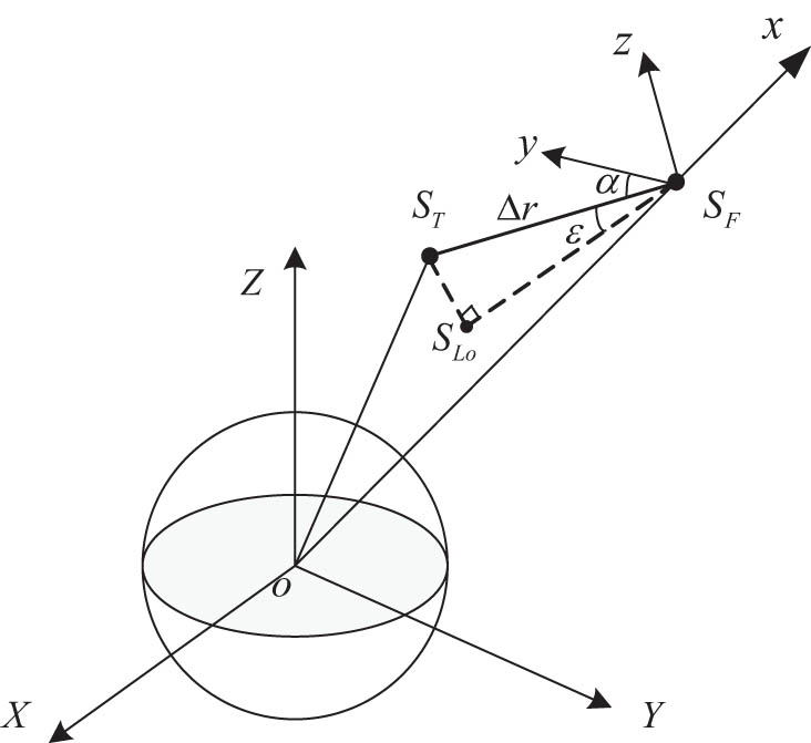
Relationship between the line-of-sight angles in a relative motion coordinate system.
This study mainly considers short-range flight-following missions in near-circular orbits, and the considered flight formation is defined as follows: (i) both the target satellite S T and follower satellite S F in the flight formation are in near-circular orbits such that the eccentricity of the two satellites is much less than 1; (ii) the follower satellite S F follows the target satellite in a close range such that the dimensionless Kepler element number of the two satellites is much less than 1.
3 Proposed relative orbital dynamics model based on the e / i vector
To address the control of near-circular short-range orbits, we introduce an e / i vector approximation to express the orbital dynamics equation. The relative eccentricity vector Δ e and relative inclination vector Δ i are defined by the following equations (D’Amico and Montenbruck et al. 2006):
where e i , i i , and Ω i (i = T, F) represent the eccentricity, orbital inclination, and right ascension of the ascending node of the target or follower satellite, respectively; θ and φ are the vector directions of Δ e and Δ i , respectively.
Following an approximate derivation, we obtain the e / i -based relative motion dynamics equations of the satellite as follows (Liu 2019):
where a F is the semi-major axis of the follower satellite; Δa = a L − a F; u is the angular amplitude; Δu = u L − u F; u 0 is the initial value of the angular amplitude. The relative motion in the orbital plane is decoupled from the relative motion in the normal direction of the orbital plane. The heading drift ellipse in the orbital plane has a semi-major axis that is twice the semi-minor axis. The difference in the eccentricities of the two satellites determines the size of the follower ellipse, and the difference in the semi-major axes of the two satellites determines the heading drift rate of the follower ellipse. This shows that by using the e / i vector, the geometric relationship of the relative motion can be described more clearly with fewer orbital elements, which is beneficial for the analysis of the orbital control of the follower formation.
4 Analysis of follower constraints and perturbation effects
Figure 1 provides a definition for the line-of-sight angle α and the deviation angle ε of the relative motion coordinate system. The constraints on the relative distance Δr, line-of-sight angle α, and deviation angle ε are as follows:
When the leader–follower satellite formation flies in low earth orbits, it is affected mainly by the aspheric J 2 perturbation of the earth and atmospheric perturbations, which prevent the constraints of the flight-following configuration from being satisfied. It is, therefore, critical to analyze these perturbations and their effects on flight-following control.
4.1 Effects of J 2 perturbations on the relative motion configuration
We shall only consider the long-term effects of a J 2 perturbation (Casalino and Forestieri 2022; Zgang and Ge 2021). According to the Gaussian perturbation equation, the rate of change in orbital elements can be expressed as follows (Yu and Jin 2010):
where R e is the radius of earth, and n is the average orbital speed. By converting Eq. (5) to the relative coordinate system shown in Figure 1 and retaining only the first-order terms in the linearization process, we obtain:
From the definition of the relative vector e / i , we obtain:
Under the influence of a J 2 perturbation, vectors Δ e and Δ i undergo the following changes:
By substituting Eqs. (8), (9), and (10) in Eq. (3), we find that the origin of the flight-following configuration changes on the y-axis, and the angle between the vectors Δ e and Δ i changes accordingly.
4.2 Effects of atmospheric drag perturbation on the relative motion configuration
Atmospheric drag is a non-conservative force. For satellite formations operating in low earth orbits, in the upper atmosphere, for extended periods of time, the micro-atmospheric drag caused by slight differences in the surface-to-mass ratio between the formations or slight differences in the satellite orbital elements under the same surface-to-mass ratio eventually accumulate (Izzo et al. 2019; Ben-Larbi et al. 2021) and cause significant effects that lead to the drift decay of the system configuration.
To analyze the effects of atmospheric drag perturbations on the system configuration, we introduced a first-order analytical solution for the atmospheric drag perturbation after introducing the average orbital elements. The average rate of change in each orbital element under the influence of atmospheric drag can then be expressed as follows (Schettino et al. 2019):
where C
D is the drag coefficient, which depends on the geometry of the satellite, variation in the altitude, and variation in the angle of attack, and it is generally set to a value of 2.2 in the calculations (Lorenzo and Andrea 2022). Additionally, K
S is the surface-to-mass ratio of the satellite,
5 Flight-following control model based on the Gaussian perturbation equation
When addressing the problem of flight-following in near-circular orbits, only the orbit of the follower satellite is controlled because the target satellite is executing a stable orbital flight without maneuvering (Sun et al. 2022). Based on the Gaussian perturbation equation, the equation of the formation control model may be rewritten as follows (Wang et al. 2021):
In this equation, Da = Δ a t − Δ a , where Δ a t is the difference between the semi-major axes of the satellites following the implementation of the control method, and Δ a is the difference between the semi-major axes of the satellites before implementing the control method. The parameters De, Di, and Du are similarly defined. Δv R, Δv T, and Δv N are the increments of the radial, tangential, and normal velocities, respectively. This simplifies the relationship between the orbital correction of the satellite in the near-circular orbit and velocity increment applied to the satellite. The above equation implies that the in-plane motion amplitude, initial phase, and drift distance along the trajectory can be varied by applying the control method in the direction of the trajectory. By applying the control method in the radial direction, the amplitude of the in-plane motion can be varied by changing the eccentricity. When the control method is applied in the direction perpendicular to the trajectory plane, the amplitude of the lateral movement can be controlled.
5.1 Control method for flight-following
5.1.1 Coarse adjustment control
Before executing the flight-following capture control technique, it is generally necessary to implement remote guidance control on the ground. The remote guidance and control terminal must maintain the follower satellite in a stable flight pattern following behind the target satellite, and the ellipse on the flight-following XY-plane must be as small as possible.
When the engine only provides a tangential thrust, it affects a, e x , and e y . For near-circular orbits, the control increments are as follows:
In this case, the satellite may drift to reduce the distance between the two satellites.
When the engine only provides a normal thrust N, there will be changes in i and Ω, but a, e x , and e y will not be affected. The control increments will therefore be:
Adjustments can be made to equalize the inclination angles of the two satellites and to approach the right ascension of the ascending node. If the two satellites are close to the right ascension of the ascending node, then in order to save fuel and to keep the ascending node’s right ascension unchanged, the pulse velocity increment should be applied over the equator to change the orbital inclination.
5.1.2 Fine adjustment control
To achieve a short-distance flight for the two satellites over a long period of time, the semi-major axes, eccentricities, and arguments of perigee of the two satellites should be as similar as possible, while satisfying the constraint conditions noted in Eq. (4). This is usually accomplished through the coordinated control of a, e, and ω. To save fuel, two pulses with the same sign are generally used to correct a, e, and ω. The position for applying the first velocity increment u 1 may be arbitrarily chosen. Once it is chosen, the magnitude of the velocity increment and the magnitude and position of the second velocity increment are fully determined as follows:
5.1.3 Hold control
When the orbits of the two satellites are in free decay and the distance between the two satellites reaches the flight-following boundary, the system should wait for the follower satellite to enter the backup control point. Backup control points are defined as the extremities, where the displacement of the follower satellite in the Z-direction of the follower coordinate system, relative to the target satellite, crosses from a positive to a negative value or from a negative to a positive value. According to Eq. (13), the increment in the tangential velocity and the position of backup control point can be maintained.
The reason for using the backup control point during orbital control is to suppress the relative value of the orbital eccentricity of the follower satellite and prevent the orbital eccentricity of the target satellite from increasing. By controlling the orbit of the follower satellite to satisfy the follower distance requirements, the orbits of the two satellites can re-enter free decay until their distance again reaches the boundary and the orbit of the follower is once again placed under control, and the cycle is then repeated.
5.2 Stability analysis of flight-following
According to the above relative orbital dynamics model and perturbation effect analysis, not only must the relative Da, De x , De y , Di, and D values between the formation satellites be controlled, the drift Du of the center of the follower must also be controlled. To address the pulse-type when considering orbit variation problems, we assume that the initial conditions of the follower satellite are t 0, r 0, and v 0, whereas the terminal conditions are t d , r d , and v d . To represent the time required for the orbit to change, the general description of the multi-pulse orbit change problem is considered as follows:
where
One out-of-plane control parameter Δv n1 is needed to make Di and D reach their target values using u 1. This process requires three in-plane controls Δv t2, Δv t3, and Δv t4 to ensure that Da, De x , De y , Di, D, and Du reach their target values using u 4. According to the actual situation, the orbit change task may be implemented using Da, De x , De y , Di, D, and Du along with the flight-following constraints.
6 Simulation examples
We conducted simulations in which the control goals of the flight formation were as follows: a following distance of R = 1 km to 3 km, line-of-sight angle of α = 0° to 45°, and deviation angle of ε = −90° to 90°. The surface-to-mass ratio of the atmospheric drag of the leading satellite was 0.044 m2/kg and that of the following satellite was 0.036 m2/kg. The initial orbit epoch Coordinated Universal Time (UTC) was 2022-02-27 00:30:00.0, and the initial states of the two satellites are shown in Table 1.
Initial orbits of the two satellites (instantaneous)
| Satellite | a (km) | E | i (°) | Ω (°) | w (°) | M (°) |
|---|---|---|---|---|---|---|
| Leader | 6860.832 | 0.001253 | 97.4866 | 270.8708 | 117.1055 | 167.3588 |
| Follower | 6859.633 | 0.001267 | 97.4961 | 270.8700 | 115.5678 | 166.3960 |
Based on the goal of achieving controlled flight-following, double pulses can be used to shorten the distance between the two satellites, while reducing the differences between the semi-major axes, eccentricities, and arguments of perigee of the two satellites. The flight-following capture control strategy of the tracking satellite is shown in Table 2.
Flight-following capture control strategy
| Orbit change sequence | Start control time (UTC) | Direction | Average control (m) | Δv (m/s) |
|---|---|---|---|---|
| 1 | March 1, 2022, 04:29:57.448 | +Y | Da = 152 | 0.084 |
| 2 | March 1, 2022, 11:18:57.551 | +Y | Da = 641 | 0.356 |
Using double-pulse control, the distance between the two satellites was approximately 17 km, eccentricity discrepancy of the two satellites was Δe = −6.0 × 10⁻⁶, right ascension of the ascending node was ΔΩ = 0.03579°, and argument of perigee was Δw = −0.22°. Figure 2 shows the variation in the relative distance between the two satellites caused by the flight-following capture control method, and Figure 3 shows the change in the line-of-sight angle of the two satellites caused by the flight-following capture control method.
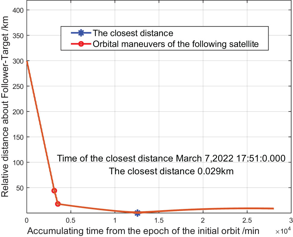
Variation in the relative distance of two satellites caused by the capture control method.
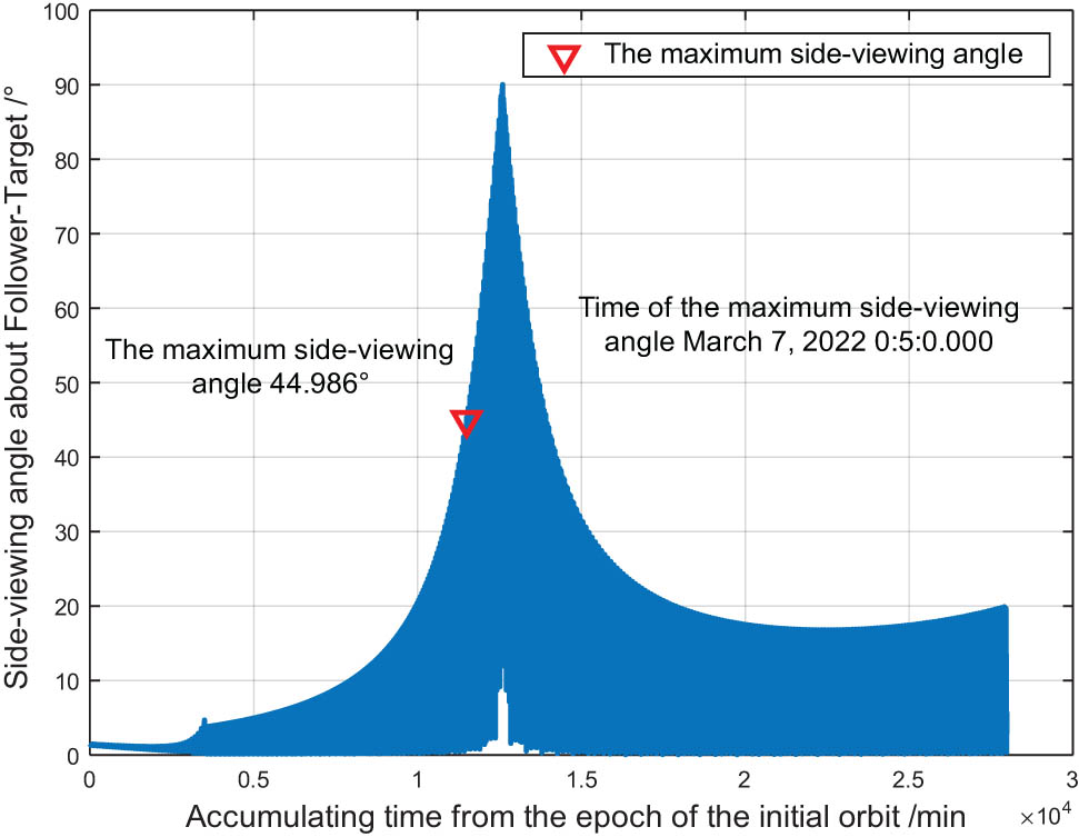
Variation in the line-of-sight angle of two satellites caused by the capture control method.
According to the evolution behavior of the binary satellites and flight-following constraints, when the two satellites reached the critical line-of-sight angle, the backup control point was calculated to raise the orbit. Afterward, the orbits of the two satellites underwent free decay again until the distance between the two satellites reached the critical value, and the backup control point was then calculated to lower the orbits. Based on this strategy, a cyclic design was carried out to form a flight-following control box. Table 3 shows a set of control strategies for the tracking satellite.
Flight-following hold control strategy
| Orbit change sequence | Start control time (UTC) | Direction | Average control (m) | Δv (m/s) |
|---|---|---|---|---|
| Line-of-sight angle is critical | March 6, 2022, 23:16:59.691 | +Y | Da = 17 | 0.009 |
| Distance is critical | March 8, 2022, 16:44:59.691 | −Y | Da = −17 | −0.009 |
Figure 3 shows that the line-of-sight angle reached a critical value at 0:5:0.00 on March 7, 2022, even though the distance between the two satellites was approximately 2.5 km. Based on Eqs. (12) and (20), the backup control point was calculated to be u = 270°, and the orbit was raised. During the process of maintaining the leader–follower relationship of the two satellites, when the relative distance between the two satellites was close to the critical value, a backup control point was calculated to be u = 90° for lowering the orbit. Figure 4 shows the variation in the relative distance of the two satellites during the flight-following control. Figure 5 shows the variation in the line-of-sight angle of the two satellites during the hold control implementation, whereas Figure 6 shows the variation in the relative in-plane distance between the two satellites during the hold control implementation.
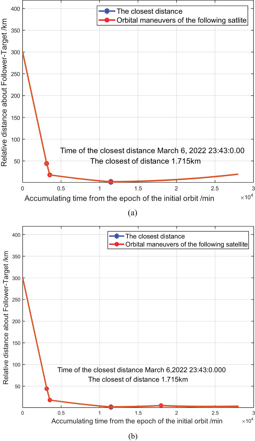
Variation in the relative distance between two satellites caused by (a) ascending orbit and (b) descending orbit during the hold control system implementation.
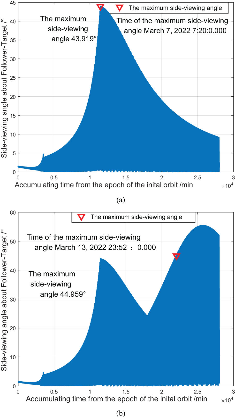
Variation in the line-of-sight angle of two satellites caused by (a) ascending orbit and (b) descending orbit during the hold control system implementation.
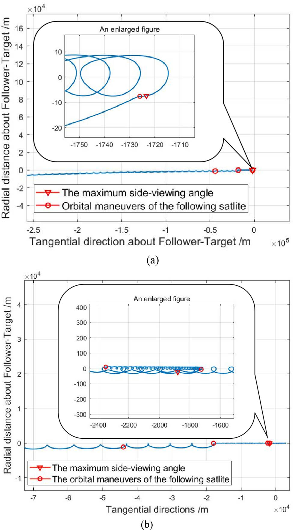
Variation in the in-plane relative distance of two satellites caused by (a) ascending orbit and (b) descending orbit during the hold control system implementation.
The analysis of the simulation process led to the following results:
When addressing a near-circular low-orbit flight-following problem, it is necessary to comprehensively consider the short-range following distance, line-of-sight angle, and deviation angle constraints. As shown in Figures 2 and 3, when the distance between the two satellites decreased, the line-of-sight angle increased. Therefore, considering only the relative following distance can adversely affect the implementation of the camera payload task.
To lower the risk of collision, the simulation step size was reduced when the height difference between the two satellites was large. This produced a more accurate real-time relative distance between the two satellites.
The simulation results further verified the e/i relative orbital dynamics model and Gaussian perturbation control model. Figure 6 shows that there was a drift ellipse in the XY-plane with a semi-major axis of 2aΔe. Furthermore, the eccentricity of the two satellites had the smallest relative value when the orbits were raised at u = 270° and lowered at u = 90°.
7 Conclusion
In this study, by elaborating upon the flight-following conditions of near-circular low-orbit satellites, we proposed a flight-following hold control box algorithm based on the e/i vector and Gaussian perturbation equation. We analyzed the effects of J 2 term and atmospheric perturbations on the relative motion configuration of this system, and we studied the flight-following hold control strategy when applied to near-circular low-orbit satellites. The simulation results showed that the algorithm of the flight-following control box is simple, meets the required flight-following conditions, and can conserve fuel.
-
Funding information: The authors state no funding involved.
-
Author contributions: All authors have accepted responsibility for the entire content of this manuscript and approved its submission.
-
Conflict of interest: The authors state no conflict of interest.
References
D’Amico S, Montenbruck O. 2006. Proximity operations of formation-flying spacecraft using an eccentricity/inclination vector separation. J Guid Control Dyn. 29(3):554–563.10.2514/1.15114Search in Google Scholar
Baranov AA, Chernov NV. 2019. Energy cost analysis to station keeping for satellite formation type “TerraSAR-X – TanDEM-X”. RUDN J Eng. 20(3):220–228.10.22363/2312-8143-2019-20-3-220-228Search in Google Scholar
Bai X, He Y, Xu M. 2021. Low-thrust reconfiguration strategy and optimization for formation flying using Jordan normal form. IEEE Trans Aerosp Electron Syst. 57(5):3279–3295.10.1109/TAES.2021.3074204Search in Google Scholar
Chen F, Dimarogonas DV. 2020. Leader–follower formation control with prescribed performance guarantees. IEEE Trans Control Netw Syst. 8(1):450–461.10.1109/TCNS.2020.3029155Search in Google Scholar
Eckstein MC, Rajasingh CK, Blumer P. 1989. Colocation strategy and collision avoidance for the geostationary satellites at 19 degrees west. International Symposium on Space Flight Dynamics; 1989 Nov 6-10; Toulouse, France. p. 55–61.Search in Google Scholar
Sharifi E, Damaren CJ. 2021. Nonlinear optimal approach to spacecraft formation flying using Lorentz and impulsive actuation. J Optim Theory Appl. 191(2):917–945.10.1007/s10957-021-01892-1Search in Google Scholar
Liu G, Cheng M, Meng Q, Tian Y, Li X. 2022. Robust fault-tolerant attitude synchronization control for formation flying satellites. Int J Adapt Control Signal Process. 36(3):503–520.10.1002/acs.3352Search in Google Scholar
Izzo D, Märtens M, Pan B. 2019. A survey on artificial intelligence trends in spacecraft guidance dynamics and control. Astrodynamics. 3(4):287–299.10.1007/s42064-018-0053-6Search in Google Scholar
Hwang J, Lee J, Park C. 2022. Collision avoidance control for formation flying of multiple spacecraft using artificial potential field. Adv Space Res. 69(5):2197–2209.10.1016/j.asr.2021.12.015Search in Google Scholar
Parsay K, Yienger K, Rowland D, Moore T, Glocer A, Garcia-Sage K. 2021. On formation flying in low earth mirrored orbits-A case study. Acta Astronaut. 184(6):142–149.10.1016/j.actaastro.2021.04.005Search in Google Scholar
Ben-Larbi MK, Jusko T, Stoll E. 2021. Input-output linearized spacecraft formation control via differential drag using relative orbital elements. Adv Space Res. 67(11):3444–3461.10.1016/j.asr.2020.12.005Search in Google Scholar
Zgang L, Ge P. 2021. High precision dynamic model and control considering J2 perturbation for spacecraft hovering in low orbit. Adv Space Res. 67(7):2185–2198.10.1016/j.asr.2021.01.015Search in Google Scholar
Casalino L, Forestieri A. 2022. Approximate optimal LEO transfers with J2 perturbation and dragsail. Acta Astronaut. 192:379–389.10.1016/j.actaastro.2021.12.006Search in Google Scholar
Liu P, Chen X, Zhao Y. 2019. Safe deployment of cluster-flying nano-satellites using relative E/I vector separation. Adv Space Res. 64(4):964–981.10.1016/j.asr.2019.05.036Search in Google Scholar
Schettino G, Alessi E, Rossi A, Valsecchi G. 2019. Exploiting dynamical perturbations for the end-of-life disposal of spacecraft in LEO. Astron Comput. 27:1–27.10.1016/j.ascom.2019.02.001Search in Google Scholar
Sun G, Zhou M, Jiang X. 2022. Non-cooperative spacecraft proximity control considering target behavior uncertainty. Astrodynamics. 6:399–411.10.1007/s42064-022-0133-5Search in Google Scholar
Wang Y, Han C, Sun X. 2021. Optimization of low-thrust Earth-orbit transfers using the vectorial orbital elements. Aerosp Sci Technol. 112(5):106614.10.1016/j.ast.2021.106614Search in Google Scholar
Lim Y, Jung Y, Bang H. 2018. Robust model predictive control for satellite formation keeping with eccentricity/inclination vector separation. Adv Space Res. 61(10):2661–2672.10.1016/j.asr.2018.02.036Search in Google Scholar
Yu BS, Jin DP. 2010. Deployment and retrieval of tethered satellite system under J2 perturbation and heating effect. Acta Astronaut. 67(7):845–853.10.1016/j.actaastro.2010.05.013Search in Google Scholar
Zhao L, Yuan C, Li X, He J. 2022. Multiple spacecraft formation flying control around artificial equilibrium point using propellantless approach. Int J Aerosp Eng. 23(1):1–26.10.1155/2022/8719645Search in Google Scholar
© 2022 Yuan Yang et al., published by De Gruyter
This work is licensed under the Creative Commons Attribution 4.0 International License.
Articles in the same Issue
- Research Articles
- Deep learning application for stellar parameters determination: I-constraining the hyperparameters
- Explaining the cuspy dark matter halos by the Landau–Ginzburg theory
- The evolution of time-dependent Λ and G in multi-fluid Bianchi type-I cosmological models
- Observational data and orbits of the comets discovered at the Vilnius Observatory in 1980–2006 and the case of the comet 322P
- Special Issue: Modern Stellar Astronomy
- Determination of the degree of star concentration in globular clusters based on space observation data
- Can local inhomogeneity of the Universe explain the accelerating expansion?
- Processing and visualisation of a series of monochromatic images of regions of the Sun
- 11-year dynamics of coronal hole and sunspot areas
- Investigation of the mechanism of a solar flare by means of MHD simulations above the active region in real scale of time: The choice of parameters and the appearance of a flare situation
- Comparing results of real-scale time MHD modeling with observational data for first flare M 1.9 in AR 10365
- Modeling of large-scale disk perturbation eclipses of UX Ori stars with the puffed-up inner disks
- A numerical approach to model chemistry of complex organic molecules in a protoplanetary disk
- Small-scale sectorial perturbation modes against the background of a pulsating model of disk-like self-gravitating systems
- Hα emission from gaseous structures above galactic discs
- Parameterization of long-period eclipsing binaries
- Chemical composition and ages of four globular clusters in M31 from the analysis of their integrated-light spectra
- Dynamics of magnetic flux tubes in accretion disks of Herbig Ae/Be stars
- Checking the possibility of determining the relative orbits of stars rotating around the center body of the Galaxy
- Photometry and kinematics of extragalactic star-forming complexes
- New triple-mode high-amplitude Delta Scuti variables
- Bubbles and OB associations
- Peculiarities of radio emission from new pulsars at 111 MHz
- Influence of the magnetic field on the formation of protostellar disks
- The specifics of pulsar radio emission
- Wide binary stars with non-coeval components
- Special Issue: The Global Space Exploration Conference (GLEX) 2021
- ANALOG-1 ISS – The first part of an analogue mission to guide ESA’s robotic moon exploration efforts
- Lunar PNT system concept and simulation results
- Special Issue: New Progress in Astrodynamics Applications - Part I
- Message from the Guest Editor of the Special Issue on New Progress in Astrodynamics Applications
- Research on real-time reachability evaluation for reentry vehicles based on fuzzy learning
- Application of cloud computing key technology in aerospace TT&C
- Improvement of orbit prediction accuracy using extreme gradient boosting and principal component analysis
- End-of-discharge prediction for satellite lithium-ion battery based on evidential reasoning rule
- High-altitude satellites range scheduling for urgent request utilizing reinforcement learning
- Performance of dual one-way measurements and precise orbit determination for BDS via inter-satellite link
- Angular acceleration compensation guidance law for passive homing missiles
- Research progress on the effects of microgravity and space radiation on astronauts’ health and nursing measures
- A micro/nano joint satellite design of high maneuverability for space debris removal
- Optimization of satellite resource scheduling under regional target coverage conditions
- Research on fault detection and principal component analysis for spacecraft feature extraction based on kernel methods
- On-board BDS dynamic filtering ballistic determination and precision evaluation
- High-speed inter-satellite link construction technology for navigation constellation oriented to engineering practice
- Integrated design of ranging and DOR signal for China's deep space navigation
- Close-range leader–follower flight control technology for near-circular low-orbit satellites
- Analysis of the equilibrium points and orbits stability for the asteroid 93 Minerva
- Access once encountered TT&C mode based on space–air–ground integration network
- Cooperative capture trajectory optimization of multi-space robots using an improved multi-objective fruit fly algorithm