Analytical study of the hybrid nanofluid for the porosity flowing through an accelerated plate: Laplace transform for the rheological behavior

Hussain Arafat; Moataz Alosaimi; Farhan Ali; Dana Mohammad Khidhir

doi:10.1515/arh-2025-0057

Article Open Access

Analytical study of the hybrid nanofluid for the porosity flowing through an accelerated plate: Laplace transform for the rheological behavior

Hussain Arafat , Moataz Alosaimi , Farhan Ali and Dana Mohammad Khidhir

Published/Copyright: November 11, 2025

Published by

Become an author with De Gruyter Brill

Author Information

From the journal Applied Rheology Volume 35 Issue 1

Abstract

This evaluation inspects an analytical computation of magneto carboxymethylcellulose (CMC)–water-based hybrid nanofluid containing molybdenum disulfide (MoS₂) and zinc oxide (ZnO) nanoparticles through an immersed porous surface. The flow is considered an exponential surface along a hybrid nanofluid. The energy and mass expression has been computed through thermal radiation, heat generation/absorption. The plate temperature obtains higher to T w , and the concentration of species C w surrounding the plate climbs linearly over time. Employing nondimensional factors allows a model’s leading equation to transform into dimensionless. The Laplace transformation methods are employed to address the nondimensional differential equations of hybrid nanofluid in the MATHEMATICA 12.0 software. The impact of developing factors on temperature, concentration, velocity, drag force, Nusselt, and Sherwood number is explored which are examined graphically and tabular form for the MoS₂ + ZnO/CMC–water and MoS₂/CMC–water. The flow variables such as porosity flow, radiative variable, heat source variable, Prandtl number, chemical reaction, and Schmidt number. It is concluded that the greater estimation of porosity and magnetic variable declined the velocity distribution for the MoS₂ + ZnO/CMC–water and MoS₂/CMC–water. Thermal radiation causes the temperature to rise distribution but declining phenomena is observed for Prandtl number. The porosity of flow and magnetic field enhances the drag force by 32.13–55.76%.

Keywords: porosity medium; nanofluid; hybrid nanofluid; thermal radiation flow; chemical reaction

Nomenclature

B 0: Magnetic field strength (−)
C *: Concentration of hybrid nanofluid (mol m⁻³)
Cf: Skin friction (−)
Ce: Chemical reaction parameter (−)
C ∞: Ambient concentration (−)
Erfc: Complementary error function (−)
g: Acceleration due to gravity (m/s²)
K 0: Porosity medium (−)
M: Magnetic field (−)
Pr: Prandtl number (−)
Q 0: Heat Sink parameter
Rd: Thermal radiation
Sc: Schmidt number
T: Temperature of the fluid (K)
t: Dimensionless time (−)
T ∞: Ambient temperature (−)
u * , v *: Velocity component (m/s)
U: Dimensionless velocity (−)
X: Coordinate horizontal to the plate (−)
Y: Coordinate normal to the plate (−)

Greek symbol

μ hnf: Coefficient of viscosity (m²/s)
v hnf: Kinematic viscosity of hyrid nanofluid (kg/ms)
ρ hnf: Density of hyrid nanofluid (kg/m³)
( ρ c p ) hnf: Specific heat of hyrid nanofluid (J/kg K)
σ *: Stefan Boltzmann constant
k hnf: Thermal conductivity of hyrid nanofluid (W/(m k))
Θ: Dimensionless temperature (−)
Φ: Dimensionless concentration (−)
γ: Porosity parameter (−)
( ϱ ): Similarity parameter (−)

Subscript

f: Base fluid
hnf: Hybrid nanoparticle
1s: Solid nanoparticle of MoS₂
2s: Solid nanoparticle of ZnO

Abbreviation

CMC: Carboxymethylcellulose
HNF: Hybrid nanofluid
MHD: Magnetohydrodynamics
TR: Thermal radiation

1 Introduction

Porosity flow is the flow of substances via a porous substance, where they pass via connected vacuums (pores). This occurrence is influenced by the material’s porosity as well as the movement of fluid within the pores. Porosity and fluid flow in porous materials are essential ideas in a variety of scientific and technical fields, particularly hydrogeology, chemical engineering, ecologic science, and material biology. Understanding the interplay between porosity and flow is crucial for accurate modeling of subsurface fluid dynamics, developing filtering systems, and maximizing recovery in hydrocarbon reservoirs. Sekhar [1] elucidated the magneto-porous time-dependent flow upon a vertical porous sheet with force convection through a Laplace transformation. Bajwa et al. [2] delineated the mechanism of porosity flow of Lorentz force past an accelerated exponential plate using an analytical solution. They noted that the magnetic field has a reducing impact on the velocity of the fluid. Khattak et al. [3] explicated the significance of Fourier heat theory embedded in a porous medium through numerical simulation. It was predicted that the temperature profile has been reduced for the larger magnitude of thermal relaxation time. Abbas et al. [4] reported the thermal slip porosity flow of viscoelastic nanomaterial immersed in a porous surface in the presence of the heat source past a slipping surface. They found that the heat transmission is enhanced by the heat source. Zeeshan et al. [5] reported the velocity effect on the nanoparticle impinging porosity sheet with nonlinear thermal radiation. It was illustrated that the velocity decayed due to the larger magnitude velocity slip effect. Jawad et al. [6] narrated the activation energy of the Maxwell nanoparticles subject to the porous flow past a stretchable sheet. They observed that the Maxwell fluid velocity augmented behavior through the numerical solution. Ahmed et al. [7] expressed the role of variable viscosity on the peristaltic nanomaterial immersed in the porous medium via numerical simulation. They noted that the porosity flow of nanofluid enhanced the reducing impact on the velocity of fluid. Pradhan et al. [8] presented the impact of heated radiation on the magneto mixed convective time-dependent flow past a porous flow via a heat source/sink considering the Laplace technique. From this analysis, the Garshof number provided the velocity goes up. Shafiq et al. [9] discussed the machine learning approach for the hybrid process of Darcy–Forchheimer flow of nanofluid past a wedge via a porous surface. They found that the escalating values of inertia coefficient and porosity medium decline the velocity of wedge. Haq et al. [10] noted the magneto flow of mixed convection in a cavity channel via a porosity surface. It was elaborated that the drag force reduces with the effect of magnetic field and mixed convection. Mahabaleshwar et al. [11] described the influence of porosity flow of viscous fluid via various conditions through the exact method.

Because of its many technical and commercial possibilities, nanofluids study has attracted significant attention from academics. Nanofluids are a significant, intriguing, and exciting topic of investigation in many technical and technological fields due to their numerous enhanced exchange of energy applications. Recent studies have shown that nanofluids transmit heat far more strongly than traditional liquids. As a result, using nanoliquids as substitutes for conventional fluids is safer. Researchers and academics have investigated the mechanical and thermal characteristics of nanofluids using a range of models. Choi [12] was the first to propose the inclusion of nanomaterials to a traditional fluid in order to increase its thermal conductivity. Aman et al. [13] discussed the thermal transportation of non-Newtonian nanoliquid, which comprises the CNTs past the various molecules. They observed that the drag force, heat, and mass transport are computed by numerical simulation. Song et al. [14] traced the effect of magnetized viscoelastic nanoliquid past a cylinder via heat generation and absorption. In this exploration, it was illustrated that the curvature variable reduces the velocity of the cylinder but enhances the temperature and concentration. Hussain et al. [15] considered the cooling features of non-Newtonian nanomaterials of chemical reactivity for the solar collector subject to the chemical reaction. It was delineated that the chemical reaction depreciates the concentration of nanomaterials. Shafiq et al. [16] illustrated the heat radiation of viscous nanofluid on the Darcy–Forchheimer flow past a stretchable sheet. It was noticed that the fluid parameter are enhanced on the machine learning process. Waqas et al. [17] observed the thermal radiative flow of nanoliquid subject to the Lorentz force within the rotating plate. Shafiq et al. [18] explained the effect of Lorentz force of simulation of microrotating nanofluid for the simulation of machine learning process. They probed that the larger estimation of micro-rotating values accelerates the drag force. Haq et al. [19] reviewed the effect of heat source on the forced convection of nanofluid subject to the chemical reaction past a tilt channel. Parmar et al. [20] explored the irreversibility exploration of magneto flow mixed convective nanofluid past a porous surface using fractional derivation solution. It was probed that the mixed convection accelerates the speed of the fluid particles. Zaheer et al. [21] inspected the stagnant point flow of the Lorentz force of nanofluid via semi-analytical solution. Bilal et al. [22] discussed the bioconvective flow of nanomaterial subject to the porosity flow and magneto dual diffusive mechanism. It was described that the porosity flow reduces the velocity of the fluid. Riaz et al. [23] computed the convective flow of viscoelastic nanofluidic in the presence of suction is influenced by triple stratification. They introduced the stratification in the thermal, concentration, and motile microorganism. Waseem et al. [24] elaborated the chemical species of nanofluid for the comparative analysis of viscoelastic fluid past an exponential sheet.

A novel fluid type known as hybrid nanofluid has recently aroused the curiosity of academics and experts. Compared to conventional nanofluids, such fluids demonstrated superior heat conduction. Whereas the standard nanofluid only includes a single kind of nanoparticle, a hybrid nanofluid has two different kinds. In order to improve the rate of thermal exchange, multiple investigators used the hybrid nanofluid models throughout their research period. Arshad et al. [25] computed the radiative flow of chemical species of the hybrid nanofluid for the rotating flow between parallel plates. They used the homotopy analysis method for the modeled equation. Shah et al. [26] discovered the microorganism effect of Prandtl hybrid nanofluid due to the chemical reaction past a stretchable sheet and illustrated that the velocity of the fluid declined due to the fluid parameter. Mishra et al. [27] performed the numerical simulation of hybrid nanofluid subject to the chemical species bioconvective mixture. In this problem, they noted that the buoyancy parameter enhanced the fluid velocity. Abbas et al. [28] obtained the effect of Marangoni convective flow condition for the buoyancy flow of tri-hybrid nanofluid subject to the heat source. They noted that the Marangoni parameter enhances the velocity of fluid and reduces the drag friction. Vijay and Sharma [29] reported the heated radiation of magneto hybrid nanofluid on the second law analysis with chemical species. It was expected that the greater magnitude of magnetic field declines the Bejan number and entropy generation. Das et al. [30] reported the chemical species of water-based hybrid nanofluid containing Cu–Al₂O₃ nanoparticles past a stretchable sheet. They observed that the larger estimation of Biot number intensifies the temperature profile. Shah et al. [31] narrated the homogenous–heterogenous chemical reaction of hybrid nanofluid subject to the tri-hybrid nanofluid past a cylinder. Jubair et al. [32] discussed the numerical simulation of hybrid nanofluid for the homogenous and heterogenous chemical species past a tilted porous cylinder. It was decided that the homogenous variable intensifies the Nusselt number. Hussain et al. [33] deliberated the dual diffusive of hybrid nanofluid immersed in a porous surface in a cavity surface. They identified that the bigger estimation of porosity flow of hybrid nanofluid decayed the velocity profile. Alqarni et al. [34] produced the mechanism flow of time-dependent squeezing flow containing Ag + TiO₂ based on blood hybrid nanofluid due to a Riga plate via the machine learning process. They detected that the nano and hybrid nanofluid accelerates the drag force for the unsteady parameter. Tassaddiq et al. [35] presented the significance of interspacing nanoparticle radius on Williamson hybrid nanofluid, the micro-squeezing surface for the Hall effect. They proved that the squeezing variable enhances the drag force for the two values of radii. Hussain et al. [36] discussed the effect of an incinerator on the micropolar hybrid nanofluid subject to the heat transportation analysis. They noted that the viscoelastic parameter influence on the drag force. Algehyne et al. [37] discussed the thermal analysis of the micropolar fluid containing hybrid nanoparticles upon a vertical sheet.

The analysis of heat radiation’s effect on the flow has gained attention for its everyday use in domains such as influence, crystal manufacturing, furnace design, and metal roll. Addressing the transfer of radiative heat is essential for designing equipment for things like nuclear reactors, turbines for gas, rockets, and atomic power plants, as numerous industrial operations involve elevated temperatures. Naqvi et al. [38] narrated the thermal radiation of second law analysis on the thermal radiation of hybrid nanofluid via numerical solution. From this analysis, they noted that the larger estimation of thermal radiation escalates the entropy generation. Reddy and Sreedevi [39] discovered the second law analysis on the thermal radiation of magento hybrid nanoflid within a square cavity. It was probed that the Lorentz reduces the velocity of the fluid. Kodi et al. [40] explained the chemical species of heated radiation of 3D rotating flow past a stretchable sheet, considering heat absorption. They obtained that the temperature enhances owing to the value of heat generation. Saleem et al. [41] described the heated radiation of hybrid nanofluid using shrinkable sheet. They exhibited that the shrinkable parameter enhances the skin friction. Naqvi et al. [42] obtained the irreversibility analysis on the hybrid nanofluid for the thermal radiation past a shrinkable sheet. It was explained that the Brikman number influences on the Bjean number for the increasing phenomena. Madhu et al. [43] explained the activated energy on thermal radiation for the hybrid nanofluid toward the stagnant surface. It was described that the activation energy parameter intensifies the concentration of nanoparticles. Gangadhar et al. [44] explained the thermodynamical analysis of the Lorentz force for the heated radiation of hybrid nanofluid-based MgO and Ag nanofluid. Ullah et al. [45] exhibited the convective flow of activated energy of heated radiation subject to the hybrid nanofluid past a stretchable sheet. In this analysis, bigger values of Biot number enhance the temperature profile. Mottupalle et al. [46] explored the heat radiation of micropolar nanofluid in the porosity flow past an oscillatory surface with bioconvection. They observed that the larger estimation of the heat radiation parameter enhances the heat transport.

Established on the works assessment, no study has been reported to produce the computation of the magnetised flow of hybrid nanofluid (MoS₂–ZnO/CMC–water) in an exponential surface impinging porous medium. This exploration communicates by studying the hybrid nanofluid in a porous medium. The thermal radiation and chemical equation have also been accounted. The fundamental equations have been transformed into non-dimensional partial differential equations by inserting non-dimensional quantities. The Laplace transformation method is used to solve the equations and determine the fluid velocity, temperature, and concentration. Graphs illustrate how flow factors affect fluid velocity, thermal distribution, and concentration. Moreover, carboxymethylcellulose (CMC–water) is considered a convectional fluid, and MoS₂–ZnO nanocomposites are added to ordinary CMC–water to improve heat and mass transmission rate. The current model is considered by applying the Laplace transforms. The final findings show the impact of physical characteristics through several plots, with a brief discussion of each graph. We tabulated the drag force, heat, and mass estimated the enhancement for hybrid nanofluid (MoS₂–ZnO). We also explored the uses of these nano-composites in CMC–water in detail.

2 Model formulation

We consider the time-dependent flow of magneto flow of CMC–water-based MoS₂ + ZnO hybrid nanofluid over a porous accelerated plate. Heat and mass computed through the expression of thermal radiative and chemical species. The y*-axis is considered vertical upward, while the x*-axis is considered horizontal. Here, an infinite plate with temperature T w and concentration C w is surrounded by the erratic flow of a viscous incompressible fluid that is initially at rest. At time t* > 0, the plate accelerates exponentially with a velocity u = u 0 exp ( a * t * ) in its own plane. The plate’s temperature rises to T w , and mass diffuses uniformly to the fluid below. A magnetic field strength B 0 is applied to the plate. Furthermore, a radiation heat flux of q r is thought to be absorbed into the plate.

Both the system of coordinates and the physical description are demonstrated graphically in Figure 1. The fluid is a CMC–water-based hybrid nanofluid that incorporates a variety of MoS₂, and ZnO nanoparticle combinations. Tables 1 and 2 list the hybrid nanoparticles’ physical characteristics.

Figure 1

Geometry of the hybrid nanofluid with porosity flow.

Table 1

Physical attributes of the nanoparticles with conventional liquid

Physical properties	C _p (J/kg K)	ρ (kg/m³)	k (W/mK)	σ (s/m)
CMC–water (<0.4%)	4,179	997.1	0.613	0.05
MoS₂	397.65	5,060	34.5	2.09 × 10⁻⁷
ZnO	495.2	5,600	13	7.261 × 10⁻⁹

Table 2

(a) Thermophysical significance of (MoS₂/CMC–water). (b) Thermophysical model for (MoS₂ + ZnO)

Properties	MoS₂/CMC–water
Viscosity ( μ )	μ nf μ f = 1 ( 1 − S 1 ) 2.5
Density ( ρ )	ρ nf ρ f = ( 1 − S 1 ) + S 1 ρ 1 s ρ f
Electric conductivity	σ nf σ f = σ 1 ( 1 + 2 S 1 ) + 2 σ f ( 1 − S 1 ) σ 1 ( 1 − S 1 ) + σ f ( 2 + S 1 )
Thermal conductivity (k)	k nf k f = k 1 + 2 k f − 2 S 1 ( k f − k 1 ) k 1 + 2 k f + S 1 ( k f − k 1 )
Heat capacity ( ρ C p )	( ρ c p ) nf ( ρ c p ) f = ( 1 − S 1 ) + S 1 ( ρ c p ) 1 s ( ρ c p ) f
Mass diffusive ( D nf )	D nf D f = ( 1 − S 1 ) − 1

Properties	MoS₂ + Zno/CMC–water
Viscosity ( μ )	μ hnf μ f = 1 ( 1 − S 1 ) 2.5 ( 1 − S 2 ) 2.5
Density ( ρ )	ρ hnf ρ f = ( 1 − S 1 ) ( 1 − S 2 ) + S 2 ρ 2 s ρ f + S 1 ρ 1 s ρ f
Electric conductivity	σ hnf σ nf = σ 2 ( 1 + 2 S 2 ) + 2 σ nf ( 1 − S 2 ) σ 2 ( 1 − S 2 ) + σ nf ( 2 + S 2 ) , σ nf σ f = σ 1 ( 1 + 2 S 1 ) + 2 σ f ( 1 − S 1 ) σ 1 ( 1 − S 1 ) + σ f ( 2 + S 1 )
Thermal conductivity (k)	k hnf k f = k s 1 + 2 k hnf − 2 S 1 ( k hnf − k 1 ) k s 1 + 2 k hnf + S 1 ( k hnf − k 1 ) × k s 2 + 2 k nf − 2 S 2 ( k nf − k s 2 ) k s 2 + 2 k nf + S 2 ( k nf − k s 2 ) k f
Heat capacity ( ρ C p )	( ρ c p ) hnf ( ρ c p ) f = ( 1 − S 1 ) ( 1 − S 2 ) + S 2 ( ρ c p ) 2 s ( ρ c p ) f + S 1 ( ρ c p ) 1 s ( ρ c p ) f
Mass diffusive ( D hnf )	D hnf D f = [ ( 1 − S 1 ) ( 1 − S 2 ) ] − 1

3 Assumption of the current flow problem

To create a realizable mathematical framework to simulate the unsteady flow of a hybrid nanofluid through a porous medium over an accelerating vertical plate, the following assumptions are made:

The hybrid nanofluid is deemed incompressible, with laminar flow throughout the domain.
Flow is assumed to be one-dimensional in the plate’s normal direction (along the y-axis), with no change in the horizontal or spanwise directions.
The physical parameters of both the base fluid and the suspended nanoparticles (such as viscosity, thermal conductivity, density, and specific heat) are assumed to be constant and unaffected by temperature or concentration.
The porous material is supposed to be homogenous and isotropic with consistent porosity and permeability.
The fluid is initially at rest. At time t > 0 t > 0, the vertical plate accelerates as a function of time. Far from the plate, the fluid velocity approaches zero.
A no-slip condition is imposed on the plate’s surface, which means that the fluid velocity precisely matches the plate’s velocity at the boundary.

The constitutive equations may be written in the boundary layer through magnetic, porosity heat radiation, and chemical reaction effects [41]

(1) ∂ u * ∂ x * + ∂ v * ∂ y * = 0 ,

(2) ∂ u * ∂ t * = μ hnf ρ hnf ∂ 2 u * ∂ y * 2 − μ hnf ρ hnf u * K 0 − σ hnf ρ hnf B 0 2 u * ,

(3) ∂ T * ∂ t * = k hnf ( ρ C p ) hnf ∂ 2 T * ∂ y * 2 − Q 0 ( T * − T ∞ ) ( ρ C p ) hnf + 16 σ * T ∞ 3 3 ( ρ C p ) hnf ,

(4) ∂ C * ∂ t * = D hnf ∂ 2 C * ∂ y * 2 − Ke ( C * − C ∞ ) .

The problem is solved analytically using the Laplace transform method under physically realistic boundary conditions

(5) t * ≤ 0 ; u * = 0 , T * = T ∞ , C * = C ∞ for all y * t * > 0 , u * = u 0 exp ( a * t * ) , T * = T ∞ + ( T w − T ∞ ) B t * C * = C ∞ + ( C w − C ∞ ) B t * at y * = 0 t * > 0 , u * = 0 , T * = T w , C * = C w at y * → ∞ ,

where B = u 0 2 ν .

Here, x and y are coordinates in terms of u * and v * velocity component, B 0 describes the magnetic field strength, ρ hnf denotes the density of the hybrid nanofluid, K 0 describes the porosity flow, σ hnf symbolized the electric conductivity of hybrid nanofluid, v hnf represents the kinematic viscosity of hybrid nanofluid, T * defines the temperature fluid, T ∞ describes far away from the temperature, C * describes the concentration, ( ρ c p ) hnf represents the heat capacity of hybrid nanofluid, t * elaborates the time, Q 0 is the rate of absorption, μ hnf is the dynamic viscosity of hybrid nanofluid, and K e is the chemical species.

The dimensionless variables are

(6) U = u * u 0 , X = x * u 0 u * , t = t * t 0 , Y = y * u 0 v * , γ = u 0 2 K 0 α f , Θ = T * − T ∞ T w − T ∞ , Rd = 16 v 2 T ∞ 3 k u o 2 , Pr = ρ v ( C p ) f k f , Ce = vK e u o 2 Φ = C * − C ∞ C w − C ∞ , Sc = v D , M = σ B 0 2 ρ u 0 2 , Q 1 = Q * v * ρ ( C p ) f u o 2 .

The molybdenum disulfide (MoS₂) and zinc oxide (ZnO) are displayed in Tables 1 and 2. The solid nanoparticles are indicated by S 1 and S 2 .

The constitution equations (1)–(4) produces

(7) ∂ U ∂ t = Π 1 ∂ 2 U ∂ Y 2 − Π 1 γ U − Π 2 MU ,

(8) ∂ Θ ∂ t = 1 Pr ∂ 2 Θ ∂ Y 2 + Π 3 Θ Rd + Π 3 Θ Q 0 ,

(9) ∂ Φ ∂ t = 1 sc ∂ 2 Φ ∂ Y 2 − K 6 Ce Φ .

Here, porosity parameter γ = v 0 K 0 a , heat sink parameter Q 0 = Q * ρ ( C p ) f u o 2 , magnetic field ( M = σ B 0 2 ρ u 0 2 ), Prandtl number Pr = μ C p k , Schmidt number Sc = v D , thermal radiation Rd = 16 v 2 T ∞ 3 k u o 2 , chemical reaction parameter Cr = vK 0 u o 2 .

The relevant boundary conditions are

(10) Φ = 0 , U = 0 , Θ = 0 , for all Y , t ≤ 0 Φ = t , U = e at , Θ = t , at Y = 0 Φ → 0 , U → 0 , Θ → 0 , as Y → ∞ ,

Dynamic viscosity = K 1 = μ hnf μ f = 1 ( 1 − S 1 ) 2.5 ( 1 − S 2 ) 2.5 ,

Density = K 2 = ρ hnf ρ f = ( 1 − S 2 ) ( 1 − S 1 ) + S 1 ρ 1 s ρ f + S 2 ρ 2 s ρ f ,

Electric conductivity K 3 = σ hnf σ nf = σ 2 ( 1 + 2 S 2 ) + 2 σ nf ( 1 − S 2 ) σ 2 ( 1 − S 2 ) + σ nf ( 2 + S 2 ) , σ nf σ f = σ 1 ( 1 + 2 S 1 ) + 2 σ f ( 1 − S 1 ) σ 1 ( 1 − S 1 ) + σ f ( 2 + S 1 ) ,

Thermal conductivity = K 4 = k hnf k f = k s 1 + 2 k hnf − 2 S 1 ( k hnf − k 1 ) k s 1 + 2 k hnf + S 1 ( k hnf − k 1 ) × k s 2 + 2 k nf − 2 S 2 ( k nf − k s 2 ) k s 2 + 2 k nf + S 2 ( k nf − k s 2 ) k f ,

Heat capacity = K 5 = ( ρ c p ) hnf ( ρ c p ) f = ( 1 − S 2 ) ( 1 − S 1 ) + S 1 ( ρ c p ) 2 s ( ρ c p ) f + S 2 ( ρ c p ) 1 s ( ρ c p ) f ,

Mass diffusion = K 6 = D hnf D f = [ ( 1 − S 1 ) ( 1 − S 2 ) ] − 1 .

4 Exact analytic solution

A function time-dependent f ( t ) may be changed into a function of complex frequency f ( s ) using the Laplace transform, a potent mathematical tool. It is particularly helpful in the processing of signals, system control analysis, and the solution of linear differential problem.

For the specified circumstances (10) the Laplace transformed technique is used precisely as following to equations (7)–(9): The flow chart for the specified analytical approach is shown in Figure 2.

(11) L ( U ) = Exp − Y Π 1 s + M 1 s − a ,

(12) L ( ϑ ) = e − Y a 1 s − d 4 s ,

(13) L ( Ω ) = e − Y Sc ( Ce + s ) s 2 .

Figure 2

Flow chart of Laplace transformation.

Equations (11)–(13) are converted via employing inverse Laplace.

4.1 Velocity profile

(14) U = e at 2 [ e − Y M 1 + Π 1 Erfc ( ϱ − M 1 + Π 1 ) + e Y M 1 + Π 1 Erfc ( ϱ + M 1 + Π 1 ) ] .

4.2 Temperature profile

(15) Θ = [ 1 4 Π 3 R 1 ⅇ − Π 3 Pr R 1 Y ( ( 2 Π 3 R 1 t − Y Pr ) ( 1 + Er f [ ϱ − Y Pr ] ) + ⅇ 2 Pr Π 3 R 1 Y ( 2 Π 3 R 1 t + Pr Y ) Erfc [ ϱ + Y Pr ] ) .

4.3 Concentration profile

(16) Φ = 1 2 ( e − y Sc ( Ce ) ) [ Erfc ( ϱ K 6 Sc ) − Sc ( K 6 Ce t ) ] + ( e y Sc ( K 6 Ce ) ) [ Erfc ( ϱ K 6 Sc ) − K 6 Sc ( Ce t ) ] .

4.4 Engineering variables

Engineering quantities are described by drag force, Nusselt, and Sherwood number

(17) Cf = ∂ U ∂ Y Y = 0 = ∂ U ∂ ϱ ϱ = 0 = 1 2 ⅇ at − 2 ⅇ − M − γ − Π 1 − Y M − γ + Π 1 π − 2 ⅇ ⅇ − M − γ − Π 1 − Y M − γ + Π 1 π ,

(18) Nu = ∂ Θ ∂ Y Y = 0 = ∂ Θ ∂ ϱ ϱ = 0 = − 2 t π ⅇ − Q Rd − PrRd a 3 t Q Rd + PrRd Π 3 − t Erfc − Q Rd + PrRd Π 3 t Q Rd + PrRd Π 3 ,

(19) Sh = ∂ Φ ∂ Y Y = 0 = ∂ Φ ∂ ϱ ϱ = 0 = − K 6 CeSc − 2 ( Sc − K 6 CeSc t ) π .

5 Results and discussion

This section focuses on the technique of the Laplace transform that is employed to address the variables defining a flow and obtain accurate analytical results regarding velocity, temperature, and concentration. A graphical analysis of the influence of multiple physical attributes on the movement of fluids was also conducted. The numerical results are displayed in graphs and tables in order to examine the properties of hybrid nanofluids along with nanofluids. The nanofluid and hybrid nanofluid in this discussion are represented by MoS₂ + ZnO/CMC–water and MoS₂/CMC–water, respectively. Drag force, heat, and mass varied depending on various physical parameters; these values are shown in Tables 3–5.

Table 3

Computation of the drag friction for the various magnitudes of a, γ, t, M

				Cf
M	γ	t	a	MoS₂/CMC–water	MoS₂ + ZnO/CMC–water
0.1				0.155331	0.160613
0.4				0.140034	0.144787
0.7				0.126255	0.130537
	0.1			0.411089	0.457303
	0.2			0.394123	0.437573
	0.3			0.373621	0.426748
		0.1		0.155332	0.206191
		1.0		0.166594	0.221141
		2.0		0.178674	0.237176
			0.1	0.269271	0.278482
			1.0	0.297592	0.307773
			2.0	0.328889	0.340134

Table 4

Computation of the Nusselt number for various magnitudes of Pr, Q ₀, t, Rd

				Nu
Pr	Q ₀	t	Rd	MoS₂/CMC–water	MoS₂ + ZnO/CMC–water
6.2				0.651454	0.668753
6.7				0.696560	0.708765
7.3				0.715656	0.728595
	0.2			0.106586	0.124346
	0.3			0.116884	0.134556
	0.4			0.125674	0.146564
		0.1		0.218736	0.248113
		0.2		0.465232	0.496226
		0.3		0.707673	0.744739
			0.1	0.817673	0.867687
			0.2	0.863627	0.898760
			0.3	0.908373	0.926538

Table 5

Exhibits variation in the Sherwood number for various magnitudes of Sc, t, Ce

			Sherwood number
Sc	t	Ce	MoS₂/CMC–water	MoS₂ + ZnO/CMC–water
1.0			0.441538	0.454456
2.0			0.405080	0.416564
3.0			0.376055	0.398575
	0.01		0.243204	0.267951
	0.02		0.236079	0.244687
	0.03		0.228081	0.234096
	0.1	1.0	0.301878	0.323535
		2.0	0.86363	0.897660
		2.5	1.086471	1.109886

Figure 3 shows the mechanism of velocity of the fluid for the variation with respect to magnetic field. A magnetic field from the outside provided transverse to the flow direction creates a Lorentz force in magnetohydrodynamics that prevents the electrically conducting fluid, in this case a nano and hybrid nanofluid. Figure 4 shows the significance of time (t) on the velocity of the fluid. It is observed that the greater estimation of the time (t) the fluid of velocity enhances near the exponential plate in the scenario of MoS₂ + ZnO and MoS₂. Figure 5 shows the velocity field with the variation of porosity medium ( γ ). Greater values of the porosity medium ( γ ) decline the velocity of the fluid in the scenario of MoS₂ + ZnO and MoS₂. Physically, the velocity profile of a hybrid nanofluid passing through a porous media is strongly influenced by the porosity parameter. The consequences of time (t) for the temperature of fluid is shown in Figure 6. The augmented flow rate enhances the effect in the scenario of MoS₂ + ZnO and MoS₂. It is a basic idea in heat transmission that is transient (time-dependent). Figure 7 shows the effect of radiation (R _d) over temperature of fluid Θ . A fluid with a larger radiation has a greater temperature of fluid, whereas a fluid with a larger heat flux has a higher temperature. The influence of heat source ( Q 0 ) over the fluid temperature Θ is shown in Figure 8. As the larger estimation of heat source variable causes the augments of fluid temperature. In thermodynamic evaluation, a value or term that denotes the source (or sink) of thermal power inside a system is called a heat source variable. The heat equation, computer simulations, or thermodynamic models where heat generation or absorption takes place can all contain it. The variation of Prandtl number against the fluid temperature Θ is shown in Figure 9. It is clear from the graphic that the thermal distribution exhibits retarding behavior as the amount of Pr increases. This occurs in thermal the physical behavior of the momentum diffusivity to thermal diffusivity ratio. This happens more frequently with MoS₂ nanofluid than MoS₂ + ZnO. The impact of the time (t) on the concentration of fluid is shown in Figure 10. The concentration of fluid is enhanced due to the larger estimation of time (t) for the scenario of MoS₂ + ZnO and MoS₂. Figure 11 depicts the influence of Schmidt number (Sc) against the concentration of fluid. Mass fluxes shift from lower to higher concentration species when the concentration of fluid grows with growing values of this variable, indicating the physical situation caused by the temperature gradient. The graph makes it clear that the chemical reaction parameter (Ce) has a substantial impact on the concentration profile as depicted in Figure 12. A rapid depreciation in the concentration of fluid occurs as chemical reaction (Ce) enhances. This mechanism is consistent with the scientific knowledge that enhanced molecular mobility brought on by greater chemical reaction (Ce) enhances mass transfer, which lowers the local fluid concentration in both MoS₂ + ZnO and MoS₂.

$Figure 3 Display of M against velocity of fluid U if γ = 0.2 , t = 0.2 , \gamma =0.2,t=0.2, S 1 = 0.01 , S 2 = 0.08 , {{\mathscr{S}}}_{1}=0.01,{{\mathscr{S}}}_{2}=0.08, Q 0 = 0.4 , Pr = 6.7 , Rd = 0.4 , Sc = 0.9 , {Q}_{0}=0.4,\Pr =6.7,{\rm{Rd}}=0.4,{\rm{Sc}}=0.9, Ce = 2.2 {\rm{Ce}}=2.2 .$

Figure 3

Display of M against velocity of fluid U if γ = 0.2 , t = 0.2 , S 1 = 0.01 , S 2 = 0.08 , Q 0 = 0.4 , Pr = 6.7 , Rd = 0.4 , Sc = 0.9 , Ce = 2.2 .

$Figure 4 Display of t t against velocity of fluid U U if γ = 0.2 , M = 0.2 , \gamma =0.2,M=0.2, S 1 = 0.01 , {{\mathscr{S}}}_{1}=0.01, S 2 = 0.08 , Q 0 = 0.4 , {{\mathscr{S}}}_{2}=0.08,{Q}_{0}=0.4, Pr = 6.7 , Rd = 0.4 , Sc = 0.9 , Ce = 2.2 \Pr =6.7,{\rm{Rd}}=0.4,{\rm{Sc}}=0.9,{\rm{Ce}}=2.2 .$

Figure 4

Display of t against velocity of fluid U if γ = 0.2 , M = 0.2 , S 1 = 0.01 , S 2 = 0.08 , Q 0 = 0.4 , Pr = 6.7 , Rd = 0.4 , Sc = 0.9 , Ce = 2.2 .

$Figure 5 Display of γ \gamma against velocity of fluid U U if t = 0.2 , M = 0.2 , t=0.2,M=0.2, S 1 = 0.01 , S 2 = 0.08 , {{\mathscr{S}}}_{1}=0.01,{{\mathscr{S}}}_{2}=0.08, Q 0 = 0.4 , Pr = 6.7 , Rd = 0.4 , Sc = 0.9 , {Q}_{0}=0.4,\Pr =6.7,{\rm{Rd}}=0.4,{\rm{Sc}}=0.9, Ce = 2.2 {\rm{Ce}}=2.2 .$

Figure 5

Display of γ against velocity of fluid U if t = 0.2 , M = 0.2 , S 1 = 0.01 , S 2 = 0.08 , Q 0 = 0.4 , Pr = 6.7 , Rd = 0.4 , Sc = 0.9 , Ce = 2.2 .

$Figure 6 Display of t t against temperature of fluid Θ \Theta if γ = 0.2 , M = 0.2 , \gamma =0.2,M=0.2, S 1 = 0.01 , S 2 = 0.08 , {{\mathscr{S}}}_{1}=0.01,{{\mathscr{S}}}_{2}=0.08, Q 0 = 0.4 , Pr = 6.7 , Rd = 0.4 , Sc = 0.9 , {Q}_{0}=0.4,\Pr =6.7,{\rm{Rd}}=0.4,{\rm{Sc}}=0.9, Ce = 2.2 {\rm{Ce}}=2.2 .$

Figure 6

Display of t against temperature of fluid Θ if γ = 0.2 , M = 0.2 , S 1 = 0.01 , S 2 = 0.08 , Q 0 = 0.4 , Pr = 6.7 , Rd = 0.4 , Sc = 0.9 , Ce = 2.2 .

$Figure 7 Display of Rd {\rm{Rd}} against temperature of fluid Θ \Theta if γ = 0.2 , M = 0.2 , \gamma =0.2,M=0.2, S 1 = 0.01 , S 2 = 0.08 , {{\mathscr{S}}}_{1}=0.01,{{\mathscr{S}}}_{2}=0.08, Q 0 = 0.4 , Pr = 6.7 , t = 0.4 , Sc = 0.9 , {Q}_{0}=0.4,\Pr =6.7,t=0.4,{\rm{Sc}}=0.9, Ce = 2.2 {\rm{Ce}}=2.2 .$

Figure 7

Display of Rd against temperature of fluid Θ if γ = 0.2 , M = 0.2 , S 1 = 0.01 , S 2 = 0.08 , Q 0 = 0.4 , Pr = 6.7 , t = 0.4 , Sc = 0.9 , Ce = 2.2 .

$Figure 8 Display of Q 0 {Q}_{0} against temperature of fluid U U if γ = 0.2 , M = 0.2 , \gamma =0.2,M=0.2, S 1 = 0.01 , S 2 = 0.08 , {{\mathscr{S}}}_{1}=0.01,{{\mathscr{S}}}_{2}=0.08, t = 0.4 , Pr = 6.7 , Rd = 0.4 , t=0.4,\Pr =6.7,{\rm{Rd}}=0.4, Sc = 0.9 , Ce = 2.2 {\rm{Sc}}=0.9,{\rm{Ce}}=2.2 .$

Figure 8

Display of Q 0 against temperature of fluid U if γ = 0.2 , M = 0.2 , S 1 = 0.01 , S 2 = 0.08 , t = 0.4 , Pr = 6.7 , Rd = 0.4 , Sc = 0.9 , Ce = 2.2 .

$Figure 9 Display of Pr \Pr against temperature of fluid Θ \Theta if γ = 0.2 , M = 0.2 , \gamma =0.2,M=0.2, S 1 = 0.01 , S 2 = 0.08 , {{\mathscr{S}}}_{1}=0.01,{{\mathscr{S}}}_{2}=0.08, t = 0.4 , Q 0 = 6.7 , Rd = 0.4 , Sc = 0.9 , t=0.4,{Q}_{0}=6.7,{\rm{Rd}}=0.4,{\rm{Sc}}=0.9, Ce = 2.2 {\rm{Ce}}=2.2 .$

Figure 9

Display of Pr against temperature of fluid Θ if γ = 0.2 , M = 0.2 , S 1 = 0.01 , S 2 = 0.08 , t = 0.4 , Q 0 = 6.7 , Rd = 0.4 , Sc = 0.9 , Ce = 2.2 .

$Figure 10 Display of t t against concentration of fluid Φ \Phi if γ = 0.2 , \gamma =0.2, M = 0.2 , M=0.2, S 1 = 0.01 , {{\mathscr{S}}}_{1}=0.01, S 2 = 0.08 , {{\mathscr{S}}}_{2}=0.08, Pr = 1.4 , Q 0 = 6.7 , \Pr =1.4,{Q}_{0}=6.7, Rd = 0.4 , {\rm{Rd}}=0.4, Sc = 0.9 , {\rm{Sc}}=0.9, Ce = 2.2 {\rm{Ce}}=2.2 .$

Figure 10

Display of t against concentration of fluid Φ if γ = 0.2 , M = 0.2 , S 1 = 0.01 , S 2 = 0.08 , Pr = 1.4 , Q 0 = 6.7 , Rd = 0.4 , Sc = 0.9 , Ce = 2.2 .

$Figure 11 Display of Sc against concentration of fluid Φ \Phi if γ = 0.2 , \gamma =0.2, M = 0.2 , S 1 = 0.01 , M=0.2,{{\mathscr{S}}}_{1}=0.01, S 2 = 0.08 , {{\mathscr{S}}}_{2}=0.08, Q 0 = 1.4 , Pr = 6.7 , {Q}_{0}=1.4,\Pr =6.7, Rd = 0.4 , {\rm{Rd}}=0.4, Sc = 0.9 , {\rm{Sc}}=0.9, Ce = 2.2 {\rm{Ce}}=2.2 .$

Figure 11

Display of Sc against concentration of fluid Φ if γ = 0.2 , M = 0.2 , S 1 = 0.01 , S 2 = 0.08 , Q 0 = 1.4 , Pr = 6.7 , Rd = 0.4 , Sc = 0.9 , Ce = 2.2 .

$Figure 12 Display of Ce against concentration of fluid U U if γ = 0.2 , \gamma =0.2, M = 0.2 , S 1 = 0.01 , M=0.2,{{\mathscr{S}}}_{1}=0.01, S 2 = 0.08 , t = 0.4 , {{\mathscr{S}}}_{2}=0.08,t=0.4, Q 0 = 6.7 , Rd = 0.4 , {Q}_{0}=6.7,{\rm{Rd}}=0.4, Rd = 0.9 , {\rm{Rd}}=0.9, Sc = 2.2 {\rm{Sc}}=2.2 .$

Figure 12

Display of Ce against concentration of fluid U if γ = 0.2 , M = 0.2 , S 1 = 0.01 , S 2 = 0.08 , t = 0.4 , Q 0 = 6.7 , Rd = 0.4 , Rd = 0.9 , Sc = 2.2 .

Figure 13 shows skin fraction under the effects of S 1 and S 2 . Greater values of γ = 0.1, 0.3, 0.5 skin friction elevated again M. The study focuses on the nanomaterials MoS₂ + ZnO and MoS₂. Figure 14 depicts the rate on transfer of heat with the influence of Rd and Q 0 . Stronger Q 0 strengthen Nusselt number. In the scenario of hybrid nanofluid nanomaterials, MoS₂ + ZnO and MoS₂ efficient behavior is examined. Plotting for changes in Sherwood number via increased Sc is shown in Figure 15. Higher estimation of Sc obtained MoS₂ + ZnO and MoS₂ by examining intensification in Sherwood number. The drag force bar plot with the variation of γ versus M is shown in Figure 16. The hybrid nanofluid was found to have maximum and minimum values of 0.45 and 0.11, respectively. The bar plot displays the highest and lowest values of the nanofluid, which are 0.4 and 0.10. Both MoS₂/CMC–water and MoS₂ + ZnO/CMC–water nanofluids’ Nusselt numbers vary with the radiation parameter Rd, as shown in Figure 17. For MoS₂/CMC–water, the heat generation/absorption parameter Q 0 ranges from 0.7 to 0.05, while for MoS₂ + ZnO/CMC–water, it ranges from 0.68 to 0.04. Figure 18 illustrates the variation of the Sherwood number with respect to the chemical reaction parameter (Ce) in the presence of the Schmidt number (Sc). For higher values of Sc, the Sherwood number for the hybrid nanofluid ranges from a maximum of 1.21 to a minimum of 0.05, while for the regular nanofluid, it ranges from 1.2 to 0.03.

$Figure 13 Display of skin friction against M M for γ \gamma if S 1 = 0.01 , S 2 = 0.08 , {{\mathscr{S}}}_{1}=0.01,{{\mathscr{S}}}_{2}=0.08, t = 0.4 , Q 0 = 6.7 , Rd = 0.4 , Rd = 0.9 , t=0.4,{Q}_{0}=6.7,{\rm{Rd}}=0.4,{\rm{Rd}}=0.9, Sc = 2.2 {\rm{Sc}}=2.2 .$

Figure 13

Display of skin friction against M for γ if S 1 = 0.01 , S 2 = 0.08 , t = 0.4 , Q 0 = 6.7 , Rd = 0.4 , Rd = 0.9 , Sc = 2.2 .

$Figure 14 Display of Nusselt number against Rd for Q 0 {Q}_{0} if S 1 = 0.01 , {{\mathscr{S}}}_{1}=0.01, S 2 = 0.08 , t = 0.4 , {{\mathscr{S}}}_{2}=0.08,t=0.4, Q 0 = 6.7 , M = 0.4 , γ = 0.9 , Sc = 2.2 {Q}_{0}=6.7,M=0.4,\gamma =0.9,{\rm{Sc}}=2.2 .$

Figure 14

Display of Nusselt number against Rd for Q 0 if S 1 = 0.01 , S 2 = 0.08 , t = 0.4 , Q 0 = 6.7 , M = 0.4 , γ = 0.9 , Sc = 2.2 .

$Figure 15 Display of Sherwood number against Ce for Sc {\rm{Sc}} if S 1 = 0.01 , {{\mathscr{S}}}_{1}=0.01, S 2 = 0.08 , t = 0.4 , {{\mathscr{S}}}_{2}=0.08,t=0.4, Q 0 = 6.7 , M = 0.4 , {Q}_{0}=6.7,M=0.4, γ = 0.9 , Rd = 0.2 \gamma =0.9,{\rm{Rd}}=0.2 .$

Figure 15

Display of Sherwood number against Ce for Sc if S 1 = 0.01 , S 2 = 0.08 , t = 0.4 , Q 0 = 6.7 , M = 0.4 , γ = 0.9 , Rd = 0.2 .

$Figure 16 Bar plot of skin friction against M M for γ \gamma if S 1 = 0.01 , S 2 = 0.08 , t = 0.4 , Q 0 = 6.7 , Rd = 0.2 , Sc = 0.1 , Ce = 0.1 {{\mathscr{S}}}_{1}=0.01,{{\mathscr{S}}}_{2}=0.08,t=0.4,{Q}_{0}=6.7,{\rm{Rd}}=0.2,{\rm{Sc}}=0.1,{\rm{Ce}}=0.1 .$

Figure 16

Bar plot of skin friction against M for γ if S 1 = 0.01 , S 2 = 0.08 , t = 0.4 , Q 0 = 6.7 , Rd = 0.2 , Sc = 0.1 , Ce = 0.1 .

$Figure 17 Bar plot of Sherwood number against Rd for Q 0 {Q}_{0} if S 1 = 0.01 , S 2 = 0.08 , t = 0.4 , M = 0.4 , {{\mathscr{S}}}_{1}=0.01,{{\mathscr{S}}}_{2}=0.08,t=0.4,M=0.4, γ = 0.9 , \gamma =0.9, Pr = 6.7 , Sc = 0.1 , Ce = 0.1 . \Pr =6.7,{\rm{Sc}}=0.1,{\rm{Ce}}=0.1.$

Figure 17

Bar plot of Sherwood number against Rd for Q 0 if S 1 = 0.01 , S 2 = 0.08 , t = 0.4 , M = 0.4 , γ = 0.9 , Pr = 6.7 , Sc = 0.1 , Ce = 0.1 .

$Figure 18 Bar plot of Sherwood number against Ce for Sc if S 1 = 0.01 , {{\mathscr{S}}}_{1}=0.01, S 2 = 0.08 , {{\mathscr{S}}}_{2}=0.08, t = 0.4 , M = 0.4 , t=0.4,M=0.4, γ = 0.9 , Pr = 6.7 , Rd = 0.1 , Q 0 = 0.1 \gamma =0.9,\Pr =6.7,{\rm{Rd}}=0.1,\hspace{1em}{Q}_{0}=0.1 .$

Figure 18

Bar plot of Sherwood number against Ce for Sc if S 1 = 0.01 , S 2 = 0.08 , t = 0.4 , M = 0.4 , γ = 0.9 , Pr = 6.7 , Rd = 0.1 , Q 0 = 0.1 .

Streamlines of the nanofluid flow with a distinct porosity parameter phase are shown in Figures 19 and 20. As the flow is affected by the porosity variable γ , the streamlines are visible. The trajectory of particles that are embedded in the liquid and carried by it is shown by the streamlines. The direction of the fluid velocity at any given location in the streamline is indicated by the tangent. The velocity boundary layer patterns with the time and without time are shown in Figures 21 and 22. A comparative analysis reveals that the time has a shearing effect upon the velocity boundary layer region based on the previously described data. The shearing effect of time and porosity parameter is caused by the resistnace of flow, which prevents fluid from moving. Figures 23 and 24 reveal the sensitivity analysis of nanoparticles volume fraction, time, magnetic field, and porosity variable.

$Figure 19 Contour sketch of nanofluid when t = 0.2 , t=0.2, S 1 = 0.01 , {{\mathscr{S}}}_{1}=0.01, S 2 = 0.0 , {{\mathscr{S}}}_{2}=0.0, γ = 0.3 , M = 0.2 \gamma =0.3,M=0.2 .$

Figure 19

Contour sketch of nanofluid when t = 0.2 , S 1 = 0.01 , S 2 = 0.0 , γ = 0.3 , M = 0.2 .

$Figure 20 Contour sketch of hybrid nanofluid when t = 0.2 , t=0.2, S 1 = 0.01 , {{\mathscr{S}}}_{1}=0.01, S 2 = 0.05 , {{\mathscr{S}}}_{2}=0.05, γ = 0.3 \gamma =0.3 .$

Figure 20

Contour sketch of hybrid nanofluid when t = 0.2 , S 1 = 0.01 , S 2 = 0.05 , γ = 0.3 .

$Figure 21 Contour sketch of hybrid nanofluid when t = 0.6 , t=0.6, S 1 = 0.01 , {{\mathscr{S}}}_{1}=0.01, S 2 = 0.05 , γ = 0.3 {{\mathscr{S}}}_{2}=0.05,\gamma =0.3 .$

Figure 21

Contour sketch of hybrid nanofluid when t = 0.6 , S 1 = 0.01 , S 2 = 0.05 , γ = 0.3 .

$Figure 22 Contour sketch of hybrid nanofluid when t = 0.2 , t=0.2, S 1 = 0.01 , {{\mathscr{S}}}_{1}=0.01, S 2 = 0.05 , γ = 0.3 {{\mathscr{S}}}_{2}=0.05,\gamma =0.3 .$

Figure 22

Contour sketch of hybrid nanofluid when t = 0.2 , S 1 = 0.01 , S 2 = 0.05 , γ = 0.3 .

$Figure 23 Sincerity analysis of volume fraction.$

Figure 23

Sincerity analysis of volume fraction.

Figure 24

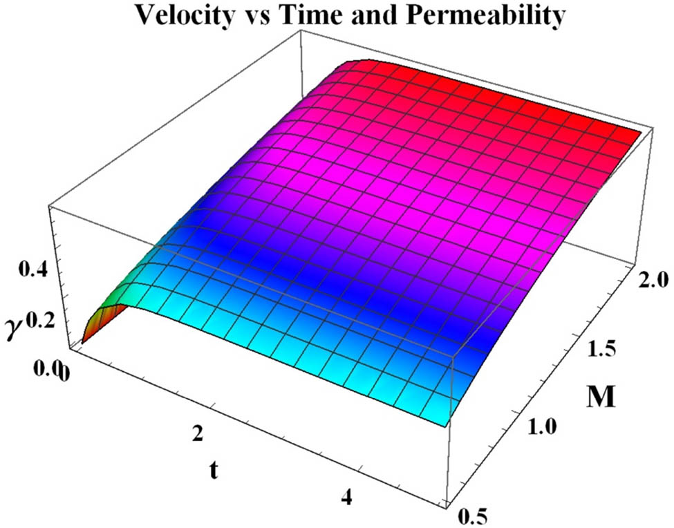
3D surface plot sincerity analysis of t, M, and γ.

Table 3 displays the skin friction coefficients that correspond to the parameters t, M, and γ. For both MoS₂ and MoS₂ + ZnO nanofluids, it has been found that rising values of γ, M, and t result in a decrease in the skin friction coefficient. The contributions of Pr, Q ₀, t, and Rd to the Nusselt number are highlighted in Table 4. For both MoS₂ and MoS₂ + ZnO, the Nusselt number is improved by increasing these parameters. The impact of Sc, Ce, and t on the Sherwood number is shown in Table 5 for both nanofluid and hybrid nanofluid scenarios. It is clear that the Sherwood number decreases with increasing values of Sc, Ce, and t. An excellent agreement was found between the Sherwood number values calculated in this work for various parameters and those reported in previous studies, as detailed in Table 6.

Table 6

Comparison of Sh for the variable of Sc, Ce, t

Sc	t	Ce	Kataria et al. [47]	Current analysis Sh
0.22	0.3	0.2	0.2956	0.2956879
	0.5		0.3866	0.3866126
	0.7		0.4632	0.4632574
0.22	0.3	2.0	0.3447	0.3447657
	0.5		0.4881	0.4881130
	0.7		0.6254	0.6254914
0.22	0.3	5.0	0.4169	0.4169134
	0.5		0.6287	0.6287364
	0.7		0.9389	0.9389432

Despite being highly respected for their effectiveness in solving differential equations, Laplace transform methods have significant drawbacks when used on complicated systems like hybrid nanofluid flows affected by heat radiation and Darcy–Forchheimer drag. These systems frequently have dynamic input functions or time-dependent boundary conditions, which the Laplace technique finds difficult to handle. The application of Laplace transforms is further complicated by the inclusion of time-varying factors or external stimuli, such as unstable heat sources, which reduces their ability to accurately capture transient characteristics. Furthermore, in hybrid nanofluid systems, the basic presumptions that underlie Laplace-based solutions might not be valid, which could result in differences between the translated analytical solutions and the real physical phenomena.

6 Conclusion

This work aims to examine the magneto-porosity flow of hybrid nanofluid past an exponential sheet. The impact of various physical parameters on nanofluid flow has been investigated. The MoS₂ and ZnO nanoparticles has been considered as hybrid nanofluid along CMC–water base fluid. This study used CMC – a low-concentration water solution (0.0–0.4%). The Laplace transformation approach provides solutions for velocity, concentration, and temperature profiles. The main result has been produced as

Strengthen the porosity variable and magnetic variable decline the velocity of hybrid nanofluid.
Velocity of the fluidic is accelerated by augmenting values of t.

Accelerating the values of heat source amplifies the temperature of the fluidic.
Larger estimation of Prandtl number deprecation of the temperature of the fluidic.
Fluidic concentration decays the (Sc) and (Ce) for augmenting.
Nanoparticles of MoS₂ and ZnO work well as a cooling energy.
Table 4 reveals an increment of heat transport enhancing the Rd, Q ₀.
The word “heat generation” refers to internal energy sources such as exothermic chemical reactions or Ohmic heating.
Furthermore, a species concentration equation is proposed to investigate coupled heat and mass transport in the presence of diffusion and potential chemical reactions, which are important in environmental engineering, catalytic processes, and biomedical flows.
Porous medium flow has a substantial impact on pressure drop, flow velocity, and heat transfer behavior in hybrid nanofluidic systems. The presence of nanoparticles changes the fluid’s consistency and particle dispersion, affecting the medium’s effective porosity.
Thermal radiation must be incorporated in heat transfer modeling in order to effectively forecast temperature distributions and improve thermal resilience. This form of heat transport becomes more dominant at high temperatures, when radiative effects outweigh conduction and convection.

6.1 Limitation of the study

The Laplace transform is an effective analytical solution approach for linear partial differential equations, especially in issues with beginning conditions. Still, the method relies on well-behaved boundary and constraining functions, which are frequently time-dependent or have a simple functional structure. As a result, the paradigm could not be directly relevant to circumstances like:

Nonlinear or arbitrary time-dependent boundary conditions, for example, oscillatory acceleration or pulsatile flow.

External forcing functions that change sporadically over time or contain discontinuities that are not easily transformable in the Laplace domain.

In such instances, other analytical or numerical techniques may be required to accurately describe the flow dynamics.

6.2 Future work

In future investigation, we consider the non-Newtonian fluid, various geometries, and the Soret and Dufor effect.

Acknowledgments

This research was supported by the Talent Project of Tianchi Young-Doctoral Program in Xinjiang Uygur Autonomous Region of China. The authors extend their appreciation to Taif University, Saudi Arabia, for supporting this work through project number (TU-DSPP-2025-05).

Funding information: This research was funded by Taif University, Saudi Arabia, Project No. (TU-DSPP-2025-05).
Author contributions: Hussain Arafat: visualization, validation, writing – review & editing, writing – original draft. Moataz Alosaimi: writing – review & editing, writing – original draft. Farhan Ali: software, conceptualization, formal analysis, investigation, methodology, writing – review & editing, writing – original draft. Dana Mohammad Khidhir: writing – original draft, supervision, software, methodology, writing – review & editing, investigation.
Conflict of interest: The authors have no conflict of interest.
Ethical approval and consent to participate: The study does not involve any ethical problem and data collection was completed in accordance with the ethical regulations.
Data availability statement: The data that support the findings of this study are available from the corresponding author.

Appendix

Π 1 = K 1 K 2 , Π 2 = K 1 K 3 , M 1 = γ + Π 2 M , Π 3 = K 4 K 5 , R 1 = Rd + Q 0 , ϱ = y 2 t .

References

[1] Sekhar KVC. Laplace transform solution of unsteady MHD Jeffry fluid flow past vertically inclined porus plate. Front Heat Mass Transf. 2021;16.10.5098/hmt.16.10Search in Google Scholar

[2] Bajwa S, Ullah S, Al-Johani AS, Khan I, Andualem M. Effects of MHD and Porosity on Jeffrey fluid flow with wall transpiration. Math Probl Eng. 2022;25:1–9.10.1155/2022/6063143Search in Google Scholar

[3] Khattak S, Ahmed M, Abrar MN, Uddin S, Sagheer M, Javeed MF, et al. Numerical simulation of Cattaneo–Christov heat flux model in a porous media past a stretching sheet. Waves Random Complex Media. 2022;9:1–20.10.1080/17455030.2022.2030503Search in Google Scholar

[4] Abbas W, Megahed AM, Ibrahim MA, Said AA. Non-Newtonian slippery nanofluid flow due to a stretching sheet through a porous medium with heat generation and thermal slip. J Nonlinear Math Phys. 2023;30(3):1221–38.10.1007/s44198-023-00125-5Search in Google Scholar

[5] Zeeshan N, Khan I, Eldin SM, Islam S, Khan MU. Two-dimensional nanofluid flow impinging on a porous stretching sheet with nonlinear thermal radiation and slip effect at the boundary enclosing energy perspective. Sci Rep. 2023;13(1):5459.10.1038/s41598-023-32650-0Search in Google Scholar PubMed PubMed Central

[6] Jawad M, Hameed MK, Nisar KS, Majeed AH. Darcy-Forchheimer flow of maxwell nanofluid flow over a porous stretching sheet with Arrhenius activation energy and nield boundary conditions. Case Stud Therm Eng. 2023;44(18):102830.10.1016/j.csite.2023.102830Search in Google Scholar

[7] Ahmed B, Nisar Z, EI‐Sherbeeny AM. Numerical study for MHD peristaltic flow of nanofluid with variable viscosity in the porous channel. ZAMM ‐ J Appl Math Mech/Z Angew Math Mech. 2023;104(3):e202300694.10.1002/zamm.202300694Search in Google Scholar

[8] Pradhan T, Jena S, Mishra SR. Laplace transformation technique for free convective time-dependent MHD flow over a vertical porous flat plate with heat sink and chemical reaction: An analytical approach. Hybrid Adv. 2024;1:100363.10.1016/j.hybadv.2024.100363Search in Google Scholar

[9] Shafiq A, Çolak AB, Sindhu TN. A hybrid approach of Buongiorno’s Law and Darcy–Forchheimer Theory using artificial neural networks: Modeling convective transport in AL2O3‐EO Mono‐Nanofluid around a Riga wedge in porous medium. Int J Numer Methods Fluids. 2024;4:299–314.10.1002/fld.5348Search in Google Scholar

[10] Haq RU, Soomro FA, Mekkaoui T, Al-Mdallal QM. MHD natural convection flow enclosure in a corrugated cavity filled with a porous medium. Int J Heat Mass Transf. 2018;121(8):1168–78.10.1016/j.ijheatmasstransfer.2018.01.063Search in Google Scholar

[11] Mahabaleshwar U, Kumar PV, Nagaraju K, Bognár G, Nayakar S. A new exact solution for the flow of a fluid through porous media for a variety of boundary conditions. Fluids. 2019;4(3):125.10.3390/fluids4030125Search in Google Scholar

[12] Choi S. Enhancing thermal conductivity of fluids with nanoparticle. In Development and applications of non-Newtonian flow, ASME, FED-Vol. 231/MD. Vol. 66; 1995. p. 99–105.10.1115/IMECE1995-0926Search in Google Scholar

[13] Aman S, Khan I, Ismail Z, Salleh MZ, Al-Mdallal QM. Heat transfer enhancement in free convection flow of CNTs Maxwell nanofluids with four different types of molecular liquids. Sci Rep. 2017;7(1):2445.10.1038/s41598-017-01358-3Search in Google Scholar PubMed PubMed Central

[14] Song YQ, Hamid A, Sun TC, Khan MI, Qayyum S, Kumar RN, et al. Unsteady mixed convection flow of magneto-Williamson nanofluid due to stretched cylinder with significant non-uniform heat source/sink features. Alex Eng J. 2021;61(1):195–206.10.1016/j.aej.2021.04.089Search in Google Scholar

[15] Hussain SM, Jamshed W, Safdar R, Shahzad F, Nasir NAAM, Ullah I. Chemical reaction and thermal characteristiecs of Maxwell nanofluid flow-through solar collector as a potential solar energy cooling application: A modified Buongiorno’s model. Energy Environ. 2022;34(5):1409–32.10.1177/0958305X221088113Search in Google Scholar

[16] Shafiq A, Çolak AB, Sindhu TN. Modeling of Darcy‐Forchheimer magnetohydrodynamic Williamson nanofluid flow towards nonlinear radiative stretching surface using artificial neural network. Int J Numer Methods Fluids. 2023;95(9):1502–20.10.1002/fld.5216Search in Google Scholar

[17] Waqas H, Naeem H, Manzoor U, Sivasankaran S, Alharbi AA, Alshomrani AS, et al. Impact of electro-magneto-hydrodynamics in radiative flow of nanofluids between two rotating plates. Alex Eng J. 2022;61(12):10307–17.10.1016/j.aej.2022.03.059Search in Google Scholar

[18] Shafiq A, Çolak AB, Sindhu TN. Optimization of micro‐rotation effect on magnetohydrodynamic nanofluid flow with artificial neural network. ZAMM ‐ J Appl Math Mech/Z Angew Math Mech. 2024;104(8):e202300498.10.1002/zamm.202300498Search in Google Scholar

[19] Haq I, Bilal M, Ahammad NA, Ghoneim ME, Ali A, Weera W. Mixed convection nanofluid flow with heat source and chemical reaction over an inclined irregular surface. ACS Omega. 2022;7(34):30477–85.10.1021/acsomega.2c03919Search in Google Scholar PubMed PubMed Central

[20] Parmar D, Kumar BVR, Murthy SVK, Kumar S. Numerical study of entropy generation in magneto-convective flow of nanofluid in porous enclosure using fractional order non-Darcian model. Phys Fluids. 2023;35(9):097142.10.1063/5.0169204Search in Google Scholar

[21] Zaheer M, Abbas SZ, Huang N, Elmasry Y. Analysis of buoyancy features on magneto hydrodynamic stagnation point flow of nanofluid using homotopy analysis method. Int J Heat Mass Transf. 2023;221:125045.10.1016/j.ijheatmasstransfer.2023.125045Search in Google Scholar

[22] Bilal S, Pan K, Hussain Z, Kada B, Pasha AA, Khan WA. Darcy-Forchheimer chemically reactive bidirectional flow of nanofluid with magneto-bioconvection and Cattaneo-Christov properties. Tribol Int. 2024;193:109313.10.1016/j.triboint.2024.109313Search in Google Scholar

[23] Riaz MB, Al-Khaled K, Adnan N, Khan SU, Ramesh K. Bioconvective triple diffusion flow of micropolar nanofluid with suction effects and convective boundary conditions. Int J Thermofluids. 2025;1:101138.10.1016/j.ijft.2025.101138Search in Google Scholar

[24] Waseem M, Hassan WH, Jawad M, Bognár G, Ghodhbani R. Examination of Chemical Reaction on Second-Grade Nanofluid and Micropolar nanofluid due to exponential stretchable sheet: A comparative study. South Afr J Chem Eng. 2025;1:373–85.10.1016/j.sajce.2025.05.010Search in Google Scholar

[25] Arshad M, Hassan A, Haider Q, Alharbi FM, Alsubaie N, Alhushaybari A, et al. Rotating hybrid nanofluid flow with chemical reaction and thermal radiation between parallel plates. Nanomaterials. 2022;12(23):4177. 10.3390/nano12234177.Search in Google Scholar PubMed PubMed Central

[26] Shah SAA, Ahammad NA, Din EM, Gamaoun F, Awan AU, Ali B. Bio-convection effects on prandtl hybrid nanofluid flow with chemical reaction and motile microorganism over a stretching sheet. Nanomaterials. 2022;12(13):2174.10.3390/nano12132174Search in Google Scholar PubMed PubMed Central

[27] Mishra NK, Anwar S, Kumam P, Seangwattana T, Bilal M, Saeed A. Numerical investigation of chemically reacting jet flow of hybrid nanofluid under the significances of bio-active mixers and chemical reaction. Heliyon. 2023;9(7):e17678.10.1016/j.heliyon.2023.e17678Search in Google Scholar PubMed PubMed Central

[28] Abbas M, Khan N, Hashmi MS, Inc M. Aspects of chemical reaction and mixed convection in ternary hybrid nanofluid with Marangoni convection and heat source. Mod Phys Lett B. 2023;38(20):2450161. 10.1142/s0217984924501616.Search in Google Scholar

[29] Vijay N, Sharma K. Entropy generation analysis in MHD hybrid nanofluid flow: Effect of thermal radiation and chemical reaction. Numer Heat Transf Part B Fundam. 2023;84(1):66–82.10.1080/10407790.2023.2186989Search in Google Scholar

[30] Das BR, Deka P, Rao S. Numerical Analysis on MHD mixed convection flow of Al2O3/H2O (Aluminum-Water) Nanofluids in a Vertical. Square Duct. East Eur J Phys. 2023;2:51–62, 10.26565/2312-4334-2023-2-02.Search in Google Scholar

[31] Shah SZH, Ayub A, Khan U, Darvesh A, Sherif ESM, Pop I. Thermal transport exploration of ternary hybrid nanofluid flow in a non-Newtonian model with homogeneous-heterogeneous chemical reactions induced by vertical cylinder. Adv Mech Eng. 2024;16(5):1–16.10.1177/16878132241252229Search in Google Scholar

[32] Jubair S, Ali B, Rafique K, Mahmood Z, Emam W. Numerical simulation of hybrid nanofluid flow with homogeneous and heterogeneous chemical reaction across an inclined permeable cylinder/plate. Energy Explor Exploit. 2024;42(6):2270–88.10.1177/01445987241272707Search in Google Scholar

[33] Hussain S, Prakash J, Almutairi B, Ramesh K. Numerical simulation of double-diffusive convection in hybrid nanofluid flow in a porous medium within a swastika-shaped cavity. Int J Numer Methods Heat Fluid Flow. 2025;35(7):2356–81. 10.1108/hff-01-2025-0062.Search in Google Scholar

[34] Alqarni MM, Mahmoud EE, Aljohani MA, Khan A, Alghamdi W, Gul T. Dynamics of time-dependent Ag and TiO2/blood Casson hybrid nanofluid squeezing flow past a Riga plate subject to an artificial neural network approach: an application to drug delivery. Mech Time-Depend Mater. 2025;29(2):49.10.1007/s11043-025-09785-wSearch in Google Scholar

[35] Tassaddiq A, Ayed H, Alghamdi S, Alghamdi W, Sulaiman M, Gul T. Cylinder coating through electromagnetic Williamson ternary hybrid nanofluid employing nanoparticle radius, and interparticle spacing effects. Int J Numer Methods Heat Fluid Flow. 2025;35(5):1543–65.10.1108/HFF-03-2025-0191Search in Google Scholar

[36] Hussain S, Jayavel P, Almutairi B, Ramesh K. Enhanced heat transfer analysis of micropolar hybrid-nanofluids in an incinerator-shaped cavity. Therm Sci Eng Prog. 2025;103471.10.1016/j.tsep.2025.103471Search in Google Scholar

[37] Algehyne EA, Lone SA, Saeed A, Bognár G. Analysis of the heat transfer enhancement in water-based micropolar hybrid nanofluid flow over a vertical flat surface. Open Phys. 2024;22(1):20230201.10.1515/phys-2023-0201Search in Google Scholar

[38] Naqvi SMRS, Waqas H, Yasmin S, Liu D, Muhammad T, Eldin SM, et al. Numerical simulations of hybrid nanofluid flow with thermal radiation and entropy generation effects. Case Stud Therm Eng. 2022;40:102479.10.1016/j.csite.2022.102479Search in Google Scholar

[39] Reddy PS, Sreedevi P. Effect of thermal radiation on heat transfer and entropy generation analysis of MHD hybrid nanofluid inside a square cavity. Waves Random Complex Media. 2022;35:412–24.10.1080/17455030.2021.2023780Search in Google Scholar

[40] Kodi R, Ravuri MR, Veeranna V, Khan MI, Abdullaev S, Tamam N. Hall current and thermal radiation effects of 3D rotating hybrid nanofluid reactive flow via stretched plate with internal heat absorption. Results Phys. 2023;53:106915.10.1016/j.rinp.2023.106915Search in Google Scholar

[41] Saleem S, Ahmad B, Naseem A, Riaz MB, Abbas T. Mono and hybrid nanofluid analysis over shrinking surface with thermal radiation: A numerical approach. Case Stud Therm Eng. 2024;54:104023.10.1016/j.csite.2024.104023Search in Google Scholar

[42] Naqvi SMRS, Manzoor U, Waqas H, Liu D, Naeem H, Eldin SM, et al. Numerical investigation of thermal radiation with entropy generation effects in hybrid nanofluid flow over a shrinking/stretching sheet. Nanotechnol Rev. 2024;13(1):20230171.10.1515/ntrev-2023-0171Search in Google Scholar

[43] Madhu J, Madhukesh JK, Sarris I, Prasannakumara BC, Ramesh GK, Shah NA, et al. Influence of quadratic thermal radiation and activation energy impacts over oblique stagnation point hybrid nanofluid flow across a cylinder. Case Stud Therm Eng. 2024;60:104624.10.1016/j.csite.2024.104624Search in Google Scholar

[44] Gangadhar K, Victoria EM, Wakif A. Irreversibility analysis for the EMHD flow of silver and magnesium oxide hybrid nanofluid due to nonlinear thermal radiation. Mod Phys Lett B. 2024. 38(33):2450337.10.1142/S0217984924503378Search in Google Scholar

[45] Ullah H, Abas SA, Fiza M, Jan AU, Akgul A, El-Rahman MA, et al. Thermal radiation effects of ternary hybrid nanofluid flow in the activation energy: Numerical computational approach. Results Eng. 2025;25:104062.10.1016/j.rineng.2025.104062Search in Google Scholar

[46] Mottupalle GR, Pobbathy D, Shankarappa B, Sanjeevamurthy A. Effects of variable fluid properties on double diffusive mixed convection with chemical reaction over an accelerating surface. Biointerface Res Appl Chem. 2021;12(4):5161–73.10.33263/BRIAC124.51615173Search in Google Scholar

[47] Kataria HR, Patel HR. Effects of chemical reaction and heat generation/absorption on magnetohydrodynamic (MHD) Casson fluid flow over an exponentially accelerated vertical plate embedded in porous medium with ramped wall temperature and ramped surface concentration. Propuls Power Res. 2019;8(1):35–46.10.1016/j.jppr.2018.12.001Search in Google Scholar

Received: 2025-04-10

Revised: 2025-08-31

Accepted: 2025-09-05

Published Online: 2025-11-11

This work is licensed under the Creative Commons Attribution 4.0 International License.

Articles in the same Issue

https://doi.org/10.1515/arh-2025-0057

Keywords for this article

porosity medium; nanofluid; hybrid nanofluid; thermal radiation flow; chemical reaction

Creative Commons

BY 4.0