Correlations for friction factor of Carreau fluids in a laminar tube flow

2.1 Pressure gradient and shear stress

Since the pressure gradient in the flow direction x, ∂ p / ∂ x , is constant over the fully developed region shown in Figure 1, the wall shear stress is described as

Figure 1

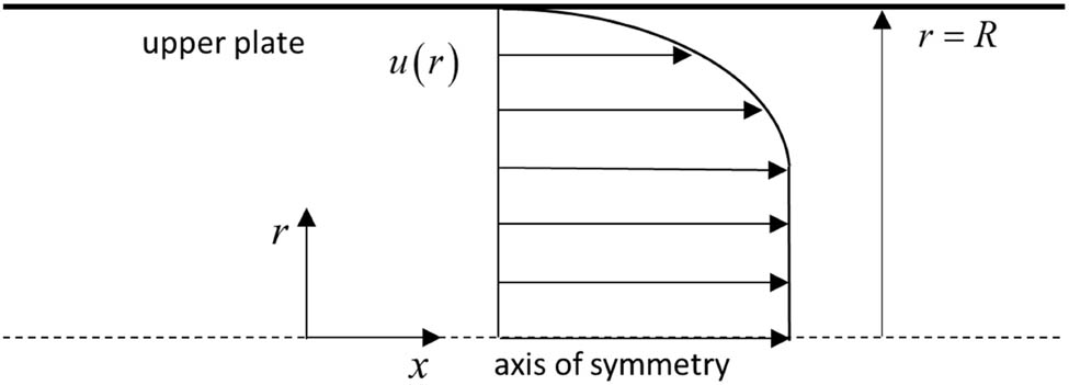
Schematic of the fully developed laminar flow in a circular, straight tube with radius R.

Then, the shear stress is

For a GNF, the shear stress is expressed as

where η is the viscosity and γ ̇ is the shear rate given by

2.2 Core flow rate

Considering the flow rate through a subsection with the radius, r, the flow rate through the subsection is expressed as

Let us define the above as the core flow rate at r. Integration of equation (5) by parts gives

Replacing equation (4) in the above equation using equation (2), q(r) is rewritten as

where the integration I 1 ( r ) is defined as [9]

Using r = τ R / τ w and d r = d τ R / τ w from equation (2), along with d u = − γ ̇ d r = − γ ̇ R / τ w ⋅ d τ from equation (4), we obtain the WRM equation

Using equation (3), equation (9) can be rewritten as

2.3 Mean velocity

At the tube wall ( r = R ), the core flow rate gives the whole flow rate, which is

The procedure given by equations (4)–(11) is called the aforementioned WRM analysis, and the details can be found in the study of Kim [9]. Now, the mean velocity is obtained by

2.4 Reynolds number

Assuming a Newtonian flow, the apparent shear rate is specified as

Then, the apparent viscosity is set as

Then, let us define the Reynolds number as

where ρ is the density of the fluid.

2.5 Darcy friction factor

The Darcy friction factor can be expressed as

which is the ratio of the wall friction force to the dynamic pressure force. Note that it is four times the Fanning friction factor. Then, the substitution of equations (14) and (15) into equation (16) gives

Then, equation (17) can be rewritten in the form of

where the shear rate ratio ϕ and the viscosity ratio ψ are

Note that f Re is the Poiseuille number. Since ϕ = ψ = 1 for a Newtonian flow, the known Newtonian–Poiseuille number is obtained as

2.6 Power law models

For a power law fluid, which remains the most significant GNF model [16], the viscosity is described by the equation

where K is the consistency and n is the index. For power law fluids, the ratios by equations (19) and (20) are represented in the form of

For n = 1 , the Newtonian value is obtained as in equation (21).

2.7 Carreau model

The viscosity using the Carreau model is expressed as [10]

where η 0 and η ∞ are the zero- and infinite-shear viscosities, respectively. Additionally, λ is the time constant. Substitution of equation (25) into equation (9) leads to [9,13]

where

Now, we are ready to calculate γ ̇ w for a specified value Q by solving equation (11) ( Q = I 1 ( γ ̇ w ) ). This will allow us to obtain an accurate value of ϕ . The nonlinearity in equation (26) is significant due to the presence of a logarithm and complex polynomials. Thus, it is essential to verify convergence with great care.

2.8 Viscosity ratio for the Carreau model

The Darcy friction factor in an actual case can be determined with the apparent shear rate by equation (18), which can be rewritten for the Carreau model as

where φ and Γ are defined as

2.9 Expressions for correlations

The Carreau fluid renders a viscosity curve, as shown in Figure 2. As shown in the figure, the viscosity behaves like a Newtonian fluid in the low shear rate regime while it behaves like a power law one in the high shear regime. For the power law model, the following identity holds:

Figure 2

Carreau viscosity model with the shear rate.

It should be noted that both d ln η p d ln γ ̇ and ϕ p are functions only of n, which is independent of K. Based on this idea, a method has been proposed to utilize this property even in more complex models. In this method, the original Carreau model can be approximated to a power law form by [1,7]

As mentioned, K 1 ( γ ̇ , η ∞ , η 0 , λ , n ) is not considered in the approximate evaluation of f, and n 1 ( γ ̇ a , η ∞ , η 0 , λ , n ) is the only function of interest. Considering equation (31), the apparent index for a specific γ ̇ a that characterizes the flow can be proposed as

For a Carreau fluid, the above relation can be rewritten as

Replacing the above quantity into equation (23), we obtain an approximate ϕ as

Since the velocity profiles by the power law and the Carreau model are different from each other, the core flow rates would be different, and thus, the friction factor. Thus, the mathematical foundation of the method seems weak and is thought to be a phenomenological methodology. Although this method yields an approximate friction factor in an efficient way, the bias from the accurate value is sometimes noticeable. To overcome this bias, this work modifies n 1 ( Γ , φ , n ) by introducing additional coefficients. The modified apparent index takes the form of

where the coefficients c , d , and h represent real numbers that vary as functions of n . The modification of Γ stems from the fact that using the apparent shear rate is largely a matter of convention, lacking a strong physical foundation. Given that linear patterns are typically observed in logarithmic plots, the error can be adjusted using the term C + d ln Γ . By setting C equal to the natural logarithm of c , we can replace Γ with c Γ d to enhance the overall accuracy of the model. Moreover, since the friction factor variation is known to change dramatically alongside φ , it is modified by a function as φ h , where the functional form h will be discussed later. This adjustment aims to better align the theoretical framework with empirical observations, providing a more robust and precise representation of the underlying physical phenomena.

As a result, we have

Then, n 2 becomes an input to equation (23) instead of n 1 . Based on the solutions using equations (26) and (27), c , d , and h will provide an accurate correlation for the friction factor of the Carreau fluid. Then, ϕ is approximated by

The resulting Poiseuille number will be obtained by

When fully expanded, the above expression gives

2.10 Coefficient determination

Since the effects of c ( n ) and d ( n ) do not cause significant changes, linear functions are sufficient to describe their relationship as follows:

The variations related to h ( n ) , however, exhibit a high degree of complexity. To accurately capture these rapid fluctuations, an exponential function is required. Through trial and error, the following equation provides an appropriate representation for h ( n ) :

The determination procedure requires a regression with the exact data. For f Re by exact calculation and n ₂ approximation to be equal, ϕ 2 ψ c ( Γ , φ , n , ϕ 2 ) = ϕ ψ c ( Γ , φ , n , ϕ ) is required and is met by ϕ 2 = ϕ . To set an optimization problem, the following normalized shear rate ratio is introduced:

Note that ϕ ( Γ i , φ j , n k ) in the above expression is obtained by solving equation (11) using equation (26). In other words,

is solved by using ϕ = γ ̇ w / γ ̇ a (equation (19)). Likewise, ϕ 2 are normalized as

Note that S 1 is expressed as

Then, the optimization problem is described as

where c = [ c 0 , c 1 , d 0 , d 1 , h 0 , h 1 , h 2 ] .

Thus, the results for validation will be presented by comparing S and S 2 . The optimization will be conducted using the generalized reduced gradient method.

3.1 Shear rate ratio

As previously discussed, the wall shear rate is used to calculate the shear rate ratio, which in turn allows for the determination of the Poiseuille number. This shear rate ratio is a critical result, providing insights into friction characteristics based on the shear rate. Figure 3 illustrates how ϕ changes with respect to n and φ . Consistent with existing research, the variation in ϕ becomes limited as n increases. Additionally, higher φ values suppress changes in ϕ and reduce the influence of n .

Figure 3

Shear rate ratio ϕ vs Γ 1 − n along with n = 0.1, 0.3, 0.5, and 0.7 for (a) φ = 0 , (b) φ = 0 .001, and (c) φ = 0.016 .

As shown in Figure 3(a), when φ = 0 , all four lines are parallel at large Γ values, the values of n decrease as Γ increases. When φ =   0.001 , as shown in Figure 3(b), the value of ϕ decreases at large Γ . Additionally, when n =   0.5 , the point where ϕ increases is delayed compared to when n =   0.7 , causing the two curves to intersect. When φ =   0.016 , the curve for n =   0.5   does not increase and remains below the curve for n =   0.7   across the entire high Γ range, as shown in Figure 3(c).

3.2 Normalization

Figure 3 shows a similarity in the patterns of change for the parameter φ for different values of n. To analyze this trend more effectively, Figure 4 presents the results after normalization. The graph displays results for 19 different n values, ranging from 0.05 to 0.95 in increments of 0.05. Each plot presents the results for φ starting from 0 and increasing 6.25 × 10 − 5 to 0.512 in doubling increments. For various engineering processes, ranging from low-velocity flows such as filtering to high-velocity flows like coating, the shear rate spans from 0.1 to 10⁵ s⁻¹. In an extreme case where λ = 10 s and n = 0, the Γ range corresponds directly to the shear rate range. Therefore, the presented result encompasses all feasible processes involving Carreau fluids.

Figure 4

S vs Γ 1 − n , with φ shown concurrently. This is presented for all examined values of n, which range from 0.5 to 0.95 in increments of 0.05. Each specific n value is indicated within its respective figure. A legend in the top left corner of the graph provides information on the color scheme used for the φ curves.

It is clear that for each n, the results change similarly with respect to φ . However, it is notable that as n increases, the point at which the decrease begins in relation to φ is delayed, as shown in Figure 4. A small value of n indicates that significant shear thinning is occurring. As n increases, there is a greater possibility that the viscosity and friction will be maintained while withstanding the influence of the solvent ( φ ≠ 0 ) . It is important to remember that the magnitude of n depends on structural changes such as alignment due to the shear rate. For a given n, the variation in φ yields interesting results. When φ is not equal to zero, the value of S increases from 0 to 1 as Γ increases and then returns to 0. Additionally, as φ increases, the change in S decreases, especially for larger values of Γ . This trend is observed in all 19 plots presented. As n increases, the increase in the curve near Γ = 1 becomes steeper, and the values gradually decrease to 0 for larger Γ . Consequently, larger values of n result in curves that are more asymmetric and skewed to the left. This result is shown in Figure 4 and will serve as base data for optimization.

Let us examine the case where n varies for the same φ . When φ = 0 , S eventually asymptotes to 1 for large values of Γ , as shown in Figure 5(a). As n increases, the curve becomes steeper and approaches 1. However, for smaller n, the increase starts at lower values of Γ . As φ increases to 0.001, S decreases towards 0 as Γ increases. In Figure 5(b), the step-like curve transforms into a bell-shaped curve for small n, but as n increases, the curve shape approaches a step function followed by a gradual decay. When φ increases to 0.016, as shown in Figure 5(c), the overall decay becomes faster, and the peaks of the curves also decrease.

Figure 5

S vs Γ 1 − n alongside n with (a) φ = 0 , (b) φ = 0.001 , and (c) φ = 0.016 . This is presented for all examined values of n, which range from 0.5 to 0.95 in increments of 0.05.

Despite the potential for minor inaccuracies in solving the nonlinear equation for wall shear rate, the propagation of errors through the friction factor and pressure drop calculations is not expected to be significantly amplified. The sensitivity of the friction factor to changes in the wall shear rate can be expressed as

where

Given that η w / η a < 1 and ∣ ( n − 1 ) λ 2 γ ̇ w 2 / ( 1 + λ 2 γ ̇ w 2 ) ∣ < 1 , the error amplification is expected to be limited. This is further supported by the observation that lim γ ̇ w → ∞ ∂ f / ∂ γ ̇ w = 0 , which is also confirmed through calculations. Consequently, the change in the friction factor can be approximated as Δ f ≈ ( ∂ f / ∂ γ ̇ w ) Δ γ ̇ w , which is likely to be suppressed. As the pressure drop is calculated based on the friction factor, its variation would also be constrained. Therefore, any numerical errors arising from the solution of the nonlinear equation (equation (11)) are not expected to significantly impact the overall results.

3.3 Coefficient determination

The optimization process specified by equation (48) using data presented in Figure 4 was conducted. The optimization yielded a set of functions with specific coefficients, which are as follows:

Upon examination, it was observed that the function values exhibit close to unity, indicating that the optimized results do not significantly diverge from the initial n 1 approximation. This consistency suggests that the optimization procedure has refined the model while maintaining its fundamental characteristics.

Figure 6 illustrates the comparison of S values calculated using equations (19), (35), and (38). The results demonstrate that the values obtained from equation (35) do not deviate significantly from those derived using equation (19), suggesting limited room for improvement in this approach. However, the graph clearly shows that equation (38) yields noticeably improved results, indicating a more effective solution to the problem at hand. When calculating the overall correlation across the entire range, both cases yield a value of 0.999. However, in the shear rate range of 1–100 s⁻¹, the n ₁ approximation results in a correlation of 0.985, while the n ₂ approximation yields 0.999. The difference becomes more pronounced when examining maximum errors. As shown in Figure 6(a), when φ =   0.001 , the maximum error decreases from 0.0783 to 0.0654, representing a 17% reduction; while, at φ = 0.016 , the error significantly decreases from 0.0656 to 0.0263, reflecting a 60% reduction. As shown in Figure 6(b), when φ =   0.001 , the error greatly decreases from 0.0852 to 0.0218, showing a 74% reduction, and at φ = 0.016 , it also significantly decreases from 0.0807 to 0.0211, again a 74% reduction. As shown in Figure 6(c), the difference is even more substantial. When φ =   0.001 , the error dramatically decreases from 0.104 to 0.018, an impressive 83% reduction; while, at φ = 0.016 , it decreases from 0.0987 to 0.0155, resulting in an 84% reduction. These results demonstrate that the n ₂ approximation generally leads to significant reductions in maximum errors across different conditions and figures.

Figure 6

S vs Γ 1 − n with φ = 0.001 , φ = 0.016 , and φ = 0.256 in (a) n = 0.1 , (b) n = 0.3 and (c) n = 0.5 . Open circles show results from equation (47), filled circles show results from equation (46), and solid lines represent the results from equation (44).

3.4 Application

In this study, the PP melt, blood flow, and solvent-based coating paste were chosen as validation cases due to their representative nature as Carreau fluids. These non-Newtonian fluids exemplify shear-thinning behavior and hold significant importance in their respective fields: polymer processing for PP melt and the coating paste and biomedical applications for blood flow. These fluids offer rich experimental datasets and cover diverse ranges of viscosity and shear rates, allowing for comprehensive model validation across different conditions.

The Carreau model effectively describes the viscosity of PP melts. Studies have shown that PP melts exhibit a secondary Newtonian plateau at extremely high shear rates, typically between 10⁶ and 10⁷, which are impractical for most processing conditions. Therefore, it is reasonable to assume that φ = 0 for PP melts in practical applications. For a specific PP melt, the Carreau constants have been determined as follows: η 0 = 936 Pa s , η ∞ = 0 Pa s , n = 0.4 , and λ = 0.207 s [17].

To illustrate the application of this model, consider the melt flow through a straight tube with a length of 1 m and a diameter of 10 mm, varying the flow rate from 10⁻⁸ to 0.001 m³/s (0.01–1,000 cm³/s). The analysis of this flow scenario yields insights into the relationship between the flow rate, friction factor, and pressure drop. As the flow rate increases from 0.01 to 1,000 cm³/s, both f and Δ p can be calculated, providing valuable information for processing considerations. It is important to note that this model does not account for shear heating, which could impact the results in real-world applications.

To account for shear heating effects, it is required to consider how viscosity changes with temperature rather than relying on an isothermal viscosity model. This consideration, however, falls outside the scope of the current study. The impact of shear heating is complex, depending on multiple fluid properties, including density, thermal conductivity, and heat capacity. As a result, it becomes challenging to validate the isothermal assumption by simply examining the total heat generation, which is typically calculated as the product of pressure drop and flow rate. A more comprehensive analysis would be required to accurately assess the significance of shear heating in the system [18]. Additionally, the Reynolds number should be verified to ensure that laminar flow conditions are maintained; in this particular case, the Re values remain well below the critical threshold for turbulent flow.

Figure 7(a) illustrates that the friction factor decreases as the flow rate increases, which is a characteristic phenomenon observed in shear-thinning fluids. As a result, the rate of pressure drop increase diminishes significantly after the inflection point of viscosity. This is associated with shear thinning, which is a result of chain alignment in polymer solutions or melts. When subjected to shear forces, the long, flexible polymer chains tend to orient themselves in the direction of flow. This alignment reduces the overall resistance to flow, leading to a decrease in viscosity as the shear rate increases [19]. Furthermore, we conducted a comparison between the pressure drop obtained through direct integration and that calculated using our proposed correlation. The figure demonstrates that these two sets of results are virtually indistinguishable, exhibiting an exceptionally close match. The root mean square error of the value obtained through correlation, compared to the value obtained through integration, is 0.023%. This high degree of agreement strongly supports the accuracy and validity of the developed correlation, effectively proving its reliability for practical applications. At a shear rate of 1,000/s, a 1% error in the wall shear rate results in errors of 1.6% in the friction factor and 0.96% in the pressure drop. In contrast, at a lower shear rate of 1 s⁻¹, the same 1% error leads to smaller errors: 0.97% in the friction factor and 0.43% in the pressure drop. These findings support the earlier assertion that the evaluation demonstrates low sensitivity to unexpected errors.

Figure 7

Pressure drop and friction factor plotted against the flow rate for (a) the PP melt [17], (b) blood [20], and (c) coating paste with solvent fractions of 1 and 4% [21]. The left vertical axis represents the pressure drop, while the right vertical axis represents friction.

As a second case, a typical human blood, which shows the secondary Newtonian plateau, is considered ( φ ≠ 0 ). A representative dataset by the Carreau model is found in ref. [20]. The model constants are η 0 = 0.056 Pa s , η ∞ = 0.00345 Pa s , n = 0.3568 , and λ = 3.313 s . In this scenario, we examine the blood flow through a tube with a length of 1 m and a diameter of 0.001 m. Figure 7(b) illustrates f and Δ p as the flow rate varies from 10 − 12 to 2.6 × 10 − 7 m³/s (0.000001–0.26 cm³/s). The upper limit of the flow rate is set to maintain laminar flow conditions. As in the previous case, the friction factor exhibits a decreasing trend with increasing flow rate. The pressure drop values calculated through integration and those obtained from the correlation show close agreement. However, unlike the previous example, there is a slight discrepancy.

Upon closer inspection of Figure 7(b), one can observe that near the inflection point, the line representing the integrated values passes slightly below the center of the circular markers, indicating the correlation-derived values. This minor deviation is a manifestation of the error that occurs in Figure 6(b). Nevertheless, from an engineering perspective, this discrepancy is negligible and does not introduce significant errors that would impact the practical use of the correlation. The root mean square error of the value derived from correlation, relative to the value from integration, is 0.34%. The level of accuracy remains sufficient for engineering applications. Overall, the results demonstrate that the proposed method can accurately predict flow characteristics for Carreau fluids.

Additionally, let us consider the case of transporting paste used for fiber coating. It is known that viscosity changes significantly depending on the solvent fraction. According to the literature, when the solvent fraction is 1%, the viscosity parameters are η 0 = 11 , 000 Pa s , η ∞ = 0.1 Pa s , n = 0.78 and λ = 1 , 500 s . When the fraction increases to 4%, η 0 and η ∞ remains the same, but n decreases to 0.41 and λ to 170 s [21]. We aim to calculate the pressure drop when transporting this paste through a 4 mm diameter pipe at various flow rates.

Figure 7(c) shows that for 1% solvent, f decreases relatively linearly, while for 4% solvent, the index decreases and an inflection occurs in f due to shear thinning. As a result, at a flow rate of 10 − 7 m 3 / s , the pressure drop for 4% solvent is more than 18 MPa lower than for 1% solvent. These calculation results prove invaluable for engineering applications, particularly in optimizing pump selection and designing efficient flow paths when provided with a specific viscosity model. The accuracy of the correlation-derived pressure drop values is noteworthy, with minimal deviations from the integration-based results. Specifically, the root mean square error is a mere 0.07% for the 1% solvent scenario and 0.13% for the 4% solvent case, demonstrating the high reliability of the correlation method in predicting pressure drops under varying solvent concentrations.

The application of this correlation is limited to the fully developed, isothermal single-phase laminar flow in straight tubes with uniform diameter, which guarantees a constant pressure gradient along the flow. It is important to note that the isothermal assumption may break down in cases of substantial shear heating, potentially resulting in viscosity reduction. Therefore, the current correlation cannot be directly applied to flows that involve transience, multiphase conditions, developments, curved geometry, compressibility [22], variable diameters, and turbulence. In addition, while it is highly unlikely that shear rates outside the range presented in this study will be considered, it should be noted that caution should be exercised when using the correlation in unusual situations where n < 0.05 or φ > 0.512, as this would constitute extrapolation beyond the validated range.

References

[1] Skelland AHP. Non-Newtonian flow and heat transfer. New York: Wiley; 1966.Suche in Google Scholar
[2] Han C. Rheology and processing of polymeric materials: Volume 1: Polymer Rheology. Oxford: Oxford University Press; 2007.10.1093/oso/9780195187823.001.0001Suche in Google Scholar
[3] Kim SK, Kazmer DO, Colon AR, Coogan TJ, Peterson AM. Non-Newtonian modeling of contact pressure in fused filament fabrication. J Rheol. 2021;65(1):27–42.10.1122/8.0000052Suche in Google Scholar
[4] Capobianchi M, Wagner D. Heat transfer in laminar flows of extended modified power law fluids in rectangular ducts. Int J Heat Mass Transf. 2010;53:558–63.10.1016/j.ijheatmasstransfer.2009.08.003Suche in Google Scholar
[5] Hong J, Kim SK, Cho YH. Flow and solidification of semi-crystalline polymer during micro-injection molding. Int J Heat Mass Transf. 2020;153:119576.10.1016/j.ijheatmasstransfer.2020.119576Suche in Google Scholar
[6] Kim SK, Kazmer DO. Non-isothermal non-Newtonian three-dimensional flow simulation of fused filament fabrication. Addit Manuf. 2022;55:102833.10.1016/j.addma.2022.102833Suche in Google Scholar
[7] Cruz DA, Coelho PM, Alves MA. A simplified method for calculating heat transfer coefficients and friction factors in laminar pipe flow of non-Newtonian fluids. J Heat Transf. 2012;134(9):091703.10.1115/1.4006288Suche in Google Scholar
[8] Kim SK. Viscosity model based on Giesekus equation. Appl Rheol. 2024;34(1):20240004.10.1515/arh-2024-0004Suche in Google Scholar
[9] Kim SK. Flow-rate based method for velocity of fully developed laminar flow in tubes. J Rheol. 2018;62:1397–407.10.1122/1.5041958Suche in Google Scholar
[10] Carreau PJ, Dekee D, Daroux M. Analysis of the viscous behavior of polymeric solutions. Can J Chem Eng. 1979;57:135–40.10.1002/cjce.5450570202Suche in Google Scholar
[11] Kim SK. Collective viscosity model for shear thinning polymeric materials. Rheol Acta. 2020;59:63–72.10.1007/s00397-019-01180-wSuche in Google Scholar
[12] Kumar M, Mondal PK. Leveraging perturbation method for the analysis of field-driven microflow of Carreau fluid. Microfluid Nanofluid. 2023;27:51.10.1007/s10404-023-02657-0Suche in Google Scholar
[13] Kim SK. Darcy friction factor and Nusselt number in laminar tube flow of Carreau fluid. Rheol Acta. 2022;61(3):243–55.10.1007/s00397-021-01317-wSuche in Google Scholar
[14] Sochi T. Analytical solutions for the flow of Carreau and Cross fluids in circular pipes and thin slits. Rheol Acta. 2015;54:745–56.10.1007/s00397-015-0863-xSuche in Google Scholar
[15] Kim SK. Correlations for convective laminar heat transfer of Carreau fluid in straight tube flow. Energies. 2022;15(7):2368.10.3390/en15072368Suche in Google Scholar
[16] Sarma R, Gaikwad H, Mondal PK. Effect of conjugate heat transfer on entropy generation in slip-driven microflow of power law fluids. Nanoscale Microsc Thermophys Eng. 2017;21(1):26–44.10.1080/15567265.2016.1272655Suche in Google Scholar
[17] Thiébaud F, Gelin JC. Characterization of rheological behaviors of polypropylene/carbon nanotubes composites and modeling their flow in a twin-screw mixer. Compos Sci Technol. 2010;70(4):647–56.10.1016/j.compscitech.2009.12.020Suche in Google Scholar
[18] Ajeeb W, Oliveira MS, Martins N, Murshed SS. Performance evaluation of convective heat transfer and laminar flow of non-Newtonian MWCNTs in a circular tube. Therm Sci Eng Prog. 2021;25:101029.10.1016/j.tsep.2021.101029Suche in Google Scholar
[19] Parisi D, Han A, Seo J, Colby RH. Rheological response of entangled isotactic polypropylene melts in strong shear flows: Edge fracture, flow curves, and normal stresses. J Rheol. 2021;65(4):605–16.10.1122/8.0000233Suche in Google Scholar
[20] ITIS Foundation. Tissue properties [Internet]. Zurich: ITIS Foundation; 2021 [cited 2025 Feb 8]. https://itis.swiss/virtual-population/tissue-properties/database/.Suche in Google Scholar
[21] Zhao X, Stylios GK, Christie RM. Rheological behavior of polymer solutions during fabric coating. J Appl Polym Sci. 2008;107:2317–21.10.1002/app.27289Suche in Google Scholar
[22] Kazmer DO, Colon AR, Peterson AM, Kim SK. Concurrent characterization of compressibility and viscosity in extrusion-based additive manufacturing of acrylonitrile butadiene styrene with fault diagnoses. Addit Manuf. 2021;46:102106.10.1016/j.addma.2021.102106Suche in Google Scholar
© 2025 the author(s), published by De Gruyter
This work is licensed under the Creative Commons Attribution 4.0 International License.
Artikel in diesem Heft
- Research Articles
- Lie symmetry analysis of bio-nano-slip flow in a conical gap between a rotating disk and cone with Stefan blowing
- Mathematical modelling of MHD hybrid nanofluid flow in a convergent and divergent channel under variable thermal conductivity effect
- Advanced ANN computational procedure for thermal transport prediction in polymer-based ternary radiative Carreau nanofluid with extreme shear rates over bullet surface
- Effects of Ca(OH)2 on mechanical damage and energy evolution characteristics of limestone adsorbed with H2S
- Effect of plasticizer content on the rheological behavior of LTCC casting slurry under large amplitude oscillating shear
- Studying the role of fine materials characteristics on the packing density and rheological properties of blended cement pastes
- Deep learning-based image analysis for confirming segregation in fresh self-consolidating concrete
- MHD Casson nanofluid flow over a three-dimensional exponentially stretching surface with waste discharge concentration: A revised Buongiorno’s model
- Rheological behavior of fire-fighting foams during their application – a new experimental set-up and protocol for foam performance qualification
- Viscoelastic characterization of corn starch paste: (II) The first normal stress difference of a cross-linked waxy corn starch paste
- An innovative rheometric tool to study chemorheology
- Effect of polymer modification on bitumen rheology: A comparative study of bitumens obtained from different sources
- Rheological and irreversibility analysis of ternary nanofluid flow over an inclined radiative MHD cylinder with porous media and couple stress
- Rheological analysis of saliva samples in the context of phonation in ectodermal dysplasia
- Analytical study of the hybrid nanofluid for the porosity flowing through an accelerated plate: Laplace transform for the rheological behavior