Sine Topp-Leone-G family of distributions: Theory and applications
-
Abdulhakim A. Al-Babtain
 and
Mohammed Elgarhy
and
Mohammed Elgarhy

Abstract
Recent studies have highlighted the statistical relevance and applicability of trigonometric distributions for the modeling of various phenomena. This paper contributes to the subject by investigating a new trigonometric family of distributions defined from the alliance of the families known as sine-G and Topp-Leone generated (TL-G), inspiring the name of sine TL-G family. The characteristics of this new family are studied through analytical, graphical and numerical approaches. Stochastic ordering and equivalence results, determination of the mode(s), some expansions of distributional functions, expressions of the quantile function and moments and basics on order statistics are discussed. In addition, we emphasize the fact that the sine TL-G family is able to generate original, simple and pliant trigonometric models for statistical purposes, beyond the capacity of the former sine-G models and other top models of the literature. This fact is revealed with the special three-parameter sine TL-G model based on the inverse Lomax model, through an efficient parametric estimation and the adjustment of two data sets of interest.
1 Introduction
In recent years, many authors have developed several ways to generate flexible continuous distributions from conventional continuous distributions. The related models have attracted statisticians of all stripes for various applications in physics, biology, medicine, finance, economy and engineering. From the mathematical point of view, these generalized distributions often belong to specific families defined from the parametric transformation of a parent cumulative distribution function (CDF). Then, the possible values of the new parameter(s) can significantly improve the statistical capabilities of the parent distribution, positively affecting the central and dispersion parameters, asymmetry, kurtosis and weight on the tails. Examples of such families are the exp-G family [35], Weibull-G family [20], Topp-Leone generated (TL-G) family [11], a new extended alpha power transformed-G [6], a new alpha power transformed-G [29], new power TL-G [17], type II general inverse exponential-G [40], truncated inverted Kumaraswamy-G [16], exponentiated truncated inverse Weibull-G [14], odd generalized NH-G [5], type II power TL-G [18] and others.
A modern approach consists in defining families of continuous distributions through the use of trigonometric transformation, parametric or not. This approach was launched by Kumar et al. [45] and Souza [67] with the use of the sine function, creating the sine-G family. On the basis of a parent continuous distribution with CDF and probability density function (PDF) given as
respectively. In addition, this trigonometric family possesses the following hazard rate function (HRF):
The advantages of the sine-G family are numerous (see [70]). One can evoke the mathematical simplicity of its probabilistic functions, its acceptable complexity of parameter(s) coinciding with that of the parent distribution, the use of the sine function makes it possible to define original trigonometric distributions through the “deformation” of any classic distribution and, in some ways, the sine-G family fills a certain lack of trigonometric distributions in the literature.
Motivated by the success of the sine-G family, several trigonometric families have seen the light, with different modeling aims. The most cited are the cos-G family by Souza et al. [67,71], sec-G family by Souza et al. [67,69], tan-G family by Souza et al. [67,68] and Ampadu [15], T-X-tan-G family by Al-Mofleh [10], N sine-G family by Mahmood et al. [50], cosine-sine-G family by Chesneau et al. [22], arcsine exponentiated-X family by Wenjing et al. [73], truncated Cauchy power-G family by Aldahlan et al. [12], sine Kumaraswamy-G family by Chesneau and Jamal [23] and TransSC-G family by Jamal and Chesneau [39].
More conventional and popular, the TL-G family studied by Al-Shomrani et al. [11] is based on a special power-polynomial transformation. From a parent continuous distribution with CDF and PDF specified by
where
The advantages of the TL-G family include the simplicity and pliancy of its functions, the following notable first-order stochastic dominance property involving the CDF of the exp-G family:
In this paper, we propose a quite logical alliance of the aforementioned two families; we develop a new family of sine generated distributions by considering the TL-G family as parent in the sine-G family. It refers to the sine Topp-Leone-G (STL-G) family. We show that the STL-G family can produce original trigonometric distributions with attractive properties, in both theoretical and practical senses. Diverse mathematical results are proved, such as stochastic ordering properties, mathematical treatment of the mode(s), manageable expansions for the PDF, expressions of characteristic measures in a tractable way and the essential theory on the model parameters based on maximization of the likelihood function. Then, after a numerical check of the efficiency of certain STL-G models through simulated data, two different data sets are considered and analyzed. As a notable applied result, we show that the STL-G models can have significantly better fits to the sine-G models defined with the same parent, and so much more models. In particular, by considering the famous bladder cancer data reported by Lee and Wang [47], we show that the special STL-G model defined with the inverse Lomax model as parent is more adequate than 21 well-referenced competitors of the literature.
The rest of the paper is organized as follows. In Section 2, the functions involved in the STL-G family are described and some special distributions are discussed. Analytical, probabilistic and statistical results of the STL-G family are provided in Section 3. The parametric inference is performed in Section 4, illustrated by a numerical study. Practical applications are developed in Section 5. Some concluding notes are proposed in Section 6.
2 The STL-G family
The presentation of the STL-G family is the object of this section.
2.1 Definition
From a parent continuous distribution with CDF and PDF specified by
Thus, it is constructed from the insertion of the CDF
As a central function, the corresponding PDF is
Among others, the characteristics and shape properties of this PDF are crucial to understand the capabilities of the related STL-G model for data fitting. As complementary reliability functions, the survival function, HRF and reversed HRF of the STL-G family are obtained as follows:
and
respectively. These functions can be involved in many mathematical treatments of the family. In particular, the shape properties of the HRF can inform on some features of the related STL-G model, as described in detail by Aarset [1].
2.2 Special three-parameter distributions of the STL-G Family
Now, we pay particular attention to the three-parameter distributions of the STL-G family defined with the following pliant parent distributions: the inverse Lomax distribution proposed by Kleiber and Kotz [43], exponentiated exponential distribution introduced by Gupta and Kundu [35] and exponentiated Lindley distribution developed by Nadarajah et al. [57]. These parent distributions are described through their CDFs and PDFs in Table 1.
Examples of three pliant distributions than can be considered as parents in the STL-G family, all with two parameters and support
| Parent distribution | Parameters | CDF (G(x)) | PDF (g(x)) |
|---|---|---|---|
| Inverse Lomax |
|
|
|
| Exponentiated exponential |
|
|
|
| Exponentiated Lindley |
|
|
|
The special distributions of the STL-G family corresponding to the parent distributions are presented in Table 1.
First special distribution: the sine Topp-Leone inverse Lomax (STLIL) distribution with CDF and PDF expressed as
and
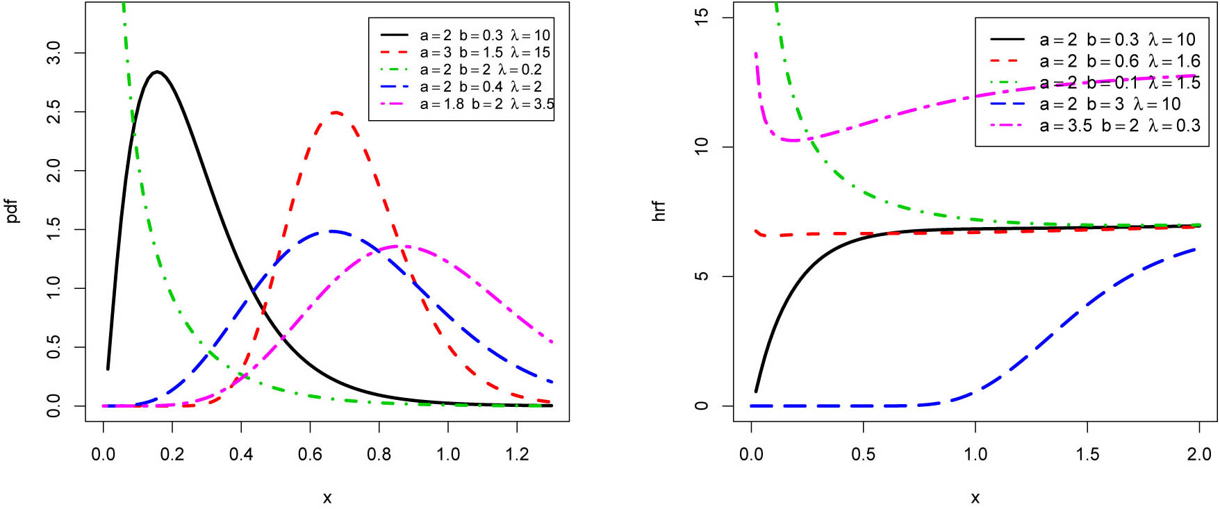
respectively. The HRF can be expressed similarly via (2.2). The STLIL distribution can also be viewed as the special distribution of the sine family taking into account the modern Topp-Leone inverse Lomax distribution studied in ref. [38] as parent. To our knowledge, the STLIL distribution is the pioneer trigonometric version of this distribution. For an illustrated analysis, Figure 1 shows the diversity of the shapes presented by

Selected curves of the PDF and HRF of the STLIL distribution.
Figure 1 shows that the STLIL distribution is unimodal. Also, “decreasing,” “plate and spike bell” shapes for
Second special distribution: the sine Topp-Leone exponentiated exponential (STLEE) distribution with CDF and PDF specified by
and
respectively. The HRF can be expressed similarly via (2.2). One can note that, when

Selected curves of the PDF and HRF of the STLEE distribution.
Figure 2 shows that the STLEE distribution is unimodal. Also, this figure reveals “decreasing” and “more or less pronounced bell” shapes for
Third special distribution: The sine Topp-Leone Lindley (STLELi) distribution with CDF and PDF defined by
and
respectively. The HRF can be expressed similarly via (2.2). Figure 3 shows the variety of shapes presented by
Selected curves of the PDF and HRF of the STLELi distribution.
Figure 3 shows “decreasing” and various “bell” shapes for
These three special distributions are evidence that the STL-G family can generate very flexible distributions, with great interest for statistical modeling. In our data analysis carried out in Section 5, we subjectively limit our attention to the STLIL model.
3 Some properties
Various properties of the STL-G family are now described, specifically stochastic ordering, equivalences, mode(s), quantile function with discussions on the skewness and kurtosis, expansion of the PDF, various moments and finally end with order statistics.
3.1 Stochastic ordering
The STL-G family satisfies the following first-order stochastic ordering properties.
Let
By applying the inequality
where
Since
where
A refinement is given by noting that
where
Hence, for given parent distribution and
3.2 Equivalences
The analysis of the equivalences of the functions of the STL-G family is of importance to understand the possibility of the related model in data fitting, mainly for the tails of the related PDF. When
When
Naturally, we see that the choice of the parent distribution is determinant for the possible limits. Also, in this regard, the parameter
As an application, in the context of the STLIL distribution defined with the inverse Lomax as parent, the following equivalences hold. When x tends to 0, we have
When x tends to
In particular, when x tends to 0 and
3.3 Mode(s)
A mode of the STL-G family, say
and
3.4 Quantile function
The inversion of
where
It is useful to understand the role of the involved parameters in the skewness; the more the shapes of
where K measures the weight of the tails; a high value for K implies heavy tails, and a small value for K implies light tails. Also, one can use
In the setting of the STLIL distribution, the quantile function can be expressed as
As illustrative examples, the Galton skewness and Moors kurtosis of the STLIL distribution are plotted in Figures 4–6.

Two dimensional plots of S and K of the STLIL distribution for

Two dimensional plots of S and K of the STLIL distribution for

Two dimensional plots of S and K of the STLIL distribution for
Figures 4–6 show that the STLIL distribution is quite right-skewed, with a varying kurtosis. For the considered values, certain monotonic structures appear, showing the versatility of these measures.
3.5 Expanded forms
Here, we derive an expansion of the PDF of the STL-G family involving transformations of the parent function. We assume that integration and differentiation term by term under the infinite sum are mathematically possible. The power series expansion for the sine function gives
By noting that
Therefore, by putting the aforementioned expansions together, we arrive at
where
and
Therefore, by differentiation with respect to x, we get
where
As a result of this manageable extended form, many mathematical properties of the STL-G family involving its PDF come directly from those of the exp-G family.
3.6 Some moments
Now, we consider an RV X having the PDF
Standard measures and functions that are written under the form
|
|
Name of
|
Usual notation |
|---|---|---|
| x | Mean |
|
|
|
Variance |
|
|
|
rth raw moment |
|
|
|
rth incomplete moment at t |
|
|
|
Moment generating function at t |
|
|
|
Characteristic function at t |
|
|
|
(Moment) skewness |
|
|
|
(Moment) kurtosis |
|
|
|
Mean deviation about
|
|
|
|
Mean deviation about
|
|
|
|
Tsallis entropy |
|
In full generality,
or, equivalently,
Such integrals can be determined by applying standard integration techniques, depending on the tractability of
knowing that the integral
where J denotes a large integer.
As application, let us consider the framework of the STLIL distribution and discuss the rth incomplete moments of X at
Obviously, the analytical calculation of this integral is unexpected. One can however envisage a numerical study if all the quantities involved are fixed. Another solution, by applying the expansion approach, is
where
where
One can derive an approximation of
3.7 Order statistics
Some basic notions on the distributional properties of the order statistics of the STL-G family are presented below. Let
where
The corresponding PDF is easily deduced as follows:
In particular, by taking
Also, by taking
From these expressions, one can envisage the determination of some characteristics of
where
Then, we have
Thus, the PDF of
where
4 Inference
Here, an inferential study of the STL-G models is proposed, including a simulation work.
4.1 Method
The inference on the parameters of the STL-G models can be carried out by using different methods. Here, we adopt the most used of all: the maximum likelihood (ML) method. The resulting estimators enjoy attractive asymptotic properties from which we can derive diverse statistical objects, such as confidence regions (including intervals) and statistical tests. The basics of the method in the setting of the STL-G models are developed below. Based on a simple random sample (SRS), let
Then, assuming that they are unique, the ML estimates are given under a vector form as
and, for any
Under some regularity assumptions, when n tends to
This result makes the construction of asymptotic confidence intervals (CIs) of the parameters possible. For any
4.2 Simulation
This section is devoted to a numerical study on the convergence of the ML estimates of the parameters of both the three-parameter STLIL and STLEE models based on SRSs. The following criteria are used: mean square errors (MSEs) and (average) CIs at the level 90% or 95%, defined with their corresponding LBs and UBs, as well as their corresponding average length (AL). The software Mathematica 9 is used. The simulation procedure takes into account the following items.
Chose the STLIL or STLEE models with selected values for
A random sample of values of size n = 50, 100, 500 and 1,000 is generated from the considered model.
For each sample, the ML estimates are computed.
Repeat items (ii) and (iii) N = 5,000 times. Then, the average ML estimates and corresponding MSEs are computed.
The CI object estimates, i.e., LBs, UBs and ALs, for the chosen parameters are also calculated with the same approach.
Numerical results are given in Tables 3 and 4 for the STLIL model and Tables 5–8 for the STLEE model.
ML estimates, MSEs and CI object estimates for the STLIL model with
| n | ML estimate | MSE | 90% | 95% | ||||
|---|---|---|---|---|---|---|---|---|
| LB | UB | AL | LB | UB | AL | |||
| 50 | 0.491 | 0.005 | 0.211 | 0.771 | 0.560 | 0.157 | 0.825 | 0.667 |
| 0.543 | 0.166 | −0.292 | 1.378 | 1.670 | −0.452 | 1.538 | 1.990 | |
| 0.583 | 0.066 | 0.323 | 0.844 | 0.521 | 0.273 | 0.893 | 0.620 | |
| 100 | 0.593 | 0.018 | 0.339 | 0.847 | 0.507 | 0.291 | 0.895 | 0.605 |
| 0.669 | 0.099 | 0.040 | 1.298 | 1.258 | −0.080 | 1.418 | 1.498 | |
| 0.489 | 0.002 | 0.366 | 0.613 | 0.247 | 0.342 | 0.637 | 0.295 | |
| 500 | 0.472 | 0.009 | 0.336 | 0.608 | 0.273 | 0.310 | 0.635 | 0.325 |
| 0.447 | 0.042 | 0.093 | 0.801 | 0.708 | 0.025 | 0.869 | 0.844 | |
| 0.525 | 0.004 | 0.415 | 0.634 | 0.219 | 0.394 | 0.655 | 0.261 | |
| 1,000 | 0.480 | 0.002 | 0.368 | 0.593 | 0.226 | 0.346 | 0.615 | 0.269 |
| 0.496 | 0.008 | 0.196 | 0.796 | 0.600 | 0.138 | 0.854 | 0.715 | |
| 0.491 | 0.002 | 0.414 | 0.569 | 0.155 | 0.399 | 0.583 | 0.184 | |
ML estimates, MSEs and CI object estimates for the STLIL model with (
| n | ML estimate | MSE | 90% | 95% | ||||
|---|---|---|---|---|---|---|---|---|
| LB | UB | AL | LB | UB | AL | |||
| 50 | 1.176 | 0.373 | 0.147 | 2.206 | 2.059 | −0.050 | 2.403 | 2.453 |
| 1.208 | 1.444 | −0.834 | 3.249 | 4.083 | −1.225 | 3.640 | 4.865 | |
| 0.974 | 0.340 | 0.140 | 1.807 | 1.667 | −0.019 | 1.967 | 1.986 | |
| 100 | 0.924 | 0.103 | 0.620 | 1.228 | 0.608 | 0.562 | 1.286 | 0.724 |
| 0.647 | 0.145 | 0.179 | 1.115 | 0.936 | 0.090 | 1.205 | 1.115 | |
| 0.829 | 0.010 | 0.639 | 1.018 | 0.379 | 0.603 | 1.055 | 0.452 | |
| 500 | 0.829 | 0.007 | 0.624 | 1.033 | 0.409 | 0.585 | 1.073 | 0.488 |
| 0.554 | 0.039 | 0.226 | 0.881 | 0.655 | 0.164 | 0.944 | 0.780 | |
| 0.810 | 0.008 | 0.658 | 0.962 | 0.304 | 0.629 | 0.991 | 0.362 | |
| 1,000 | 0.821 | 0.003 | 0.702 | 0.939 | 0.238 | 0.679 | 0.962 | 0.283 |
| 0.529 | 0.008 | 0.347 | 0.710 | 0.362 | 0.313 | 0.745 | 0.432 | |
| 0.803 | 0.001 | 0.715 | 0.890 | 0.175 | 0.699 | 0.907 | 0.208 | |
ML estimates, MSEs and CI object estimates for the STLEE model with
| n | ML estimate | MSE | 90% | 95% | ||||
|---|---|---|---|---|---|---|---|---|
| LB | UB | AL | LB | UB | AL | |||
| 50 | 0.547 | 0.021 | 0.325 | 0.768 | 0.443 | 0.283 | 0.811 | 0.528 |
| 0.513 | 0.112 | 0.011 | 1.015 | 1.004 | −0.085 | 1.111 | 1.197 | |
| 0.543 | 0.007 | 0.395 | 0.691 | 0.297 | 0.366 | 0.720 | 0.353 | |
| 100 | 0.570 | 0.014 | 0.395 | 0.745 | 0.350 | 0.362 | 0.779 | 0.417 |
| 0.639 | 0.133 | 0.171 | 1.107 | 0.936 | 0.082 | 1.197 | 1.115 | |
| 0.506 | 0.004 | 0.410 | 0.603 | 0.193 | 0.391 | 0.621 | 0.230 | |
| 500 | 0.524 | 0.003 | 0.398 | 0.650 | 0.252 | 0.374 | 0.674 | 0.300 |
| 0.559 | 0.026 | 0.226 | 0.893 | 0.667 | 0.162 | 0.956 | 0.794 | |
| 0.495 | 0.002 | 0.419 | 0.571 | 0.152 | 0.404 | 0.585 | 0.181 | |
| 1,000 | 0.479 | 0.002 | 0.394 | 0.564 | 0.170 | 0.378 | 0.580 | 0.203 |
| 0.474 | 0.012 | 0.256 | 0.692 | 0.436 | 0.214 | 0.734 | 0.519 | |
| 0.499 | 0.001 | 0.439 | 0.560 | 0.121 | 0.427 | 0.572 | 0.145 | |
ML estimates, MSEs and CI object estimates for the STLEE model with
| n | ML estimate | MSE | 90% | 95% | ||||
|---|---|---|---|---|---|---|---|---|
| LB | UB | AL | LB | UB | AL | |||
| 50 | 0.893 | 0.181 | 0.331 | 1.455 | 1.124 | 0.223 | 1.563 | 1.339 |
| 0.533 | 0.243 | −0.134 | 1.201 | 1.335 | −0.262 | 1.329 | 1.590 | |
| 0.586 | 0.040 | 0.407 | 0.765 | 0.358 | 0.372 | 0.799 | 0.427 | |
| 100 | 0.956 | 0.038 | 0.578 | 1.333 | 0.755 | 0.506 | 1.405 | 0.900 |
| 0.573 | 0.057 | 0.141 | 1.004 | 0.863 | 0.059 | 1.087 | 1.028 | |
| 0.516 | 0.003 | 0.426 | 0.606 | 0.181 | 0.408 | 0.624 | 0.215 | |
| 500 | 0.916 | 0.020 | 0.637 | 1.195 | 0.559 | 0.583 | 1.249 | 0.665 |
| 0.494 | 0.024 | 0.206 | 0.782 | 0.577 | 0.150 | 0.837 | 0.687 | |
| 0.513 | 0.002 | 0.448 | 0.598 | 0.150 | 0.434 | 0.612 | 0.178 | |
| 1,000 | 0.958 | 0.019 | 0.720 | 1.196 | 0.475 | 0.675 | 1.241 | 0.567 |
| 0.543 | 0.014 | 0.288 | 0.799 | 0.512 | 0.239 | 0.848 | 0.610 | |
| 0.503 | 0.001 | 0.448 | 0.558 | 0.110 | 0.438 | 0.569 | 0.131 | |
ML estimates, MSEs and CI object estimates for the STLEE model with
| n | ML estimate | MSE | 90% | 95% | ||||
|---|---|---|---|---|---|---|---|---|
| LB | UB | AL | LB | UB | AL | |||
| 50 | 0.487 | 0.008 | 0.355 | 0.620 | 0.264 | 0.330 | 0.645 | 0.315 |
| 0.156 | 0.027 | −0.041 | 0.353 | 0.394 | −0.079 | 0.391 | 0.469 | |
| 1.382 | 0.231 | 0.359 | 2.406 | 2.046 | 0.163 | 2.602 | 2.438 | |
| 100 | 0.500 | 0.001 | 0.407 | 0.593 | 0.186 | 0.389 | 0.611 | 0.222 |
| 0.119 | 0.003 | 0.003 | 0.234 | 0.231 | −0.019 | 0.256 | 0.275 | |
| 1.415 | 0.136 | 0.756 | 2.074 | 1.319 | 0.629 | 2.201 | 1.571 | |
| 500 | 0.481 | 0.002 | 0.409 | 0.554 | 0.145 | 0.395 | 0.568 | 0.173 |
| 0.094 | 0.003 | 0.009 | 0.180 | 0.172 | −0.008 | 0.197 | 0.204 | |
| 1.422 | 0.089 | 0.857 | 1.988 | 1.130 | 0.749 | 2.096 | 1.347 | |
| 1,000 | 0.497 | 0.000 | 0.438 | 0.557 | 0.120 | 0.426 | 0.569 | 0.143 |
| 0.106 | 0.001 | 0.076 | 0.235 | 0.159 | 0.061 | 0.250 | 0.189 | |
| 1.158 | 0.009 | 0.920 | 1.396 | 0.476 | 0.874 | 1.441 | 0.567 | |
ML estimates, MSEs and CI object estimates for the STLEE model with
| n | ML estimate | MSE | 90% | 95% | ||||
|---|---|---|---|---|---|---|---|---|
| LB | UB | AL | LB | UB | AL | |||
| 50 | 1.771 | 0.523 | 0.711 | 2.831 | 2.120 | 0.508 | 3.034 | 2.526 |
| 0.642 | 0.198 | −0.072 | 1.356 | 1.428 | −0.209 | 1.493 | 1.702 | |
| 1.715 | 0.654 | 0.676 | 2.755 | 2.080 | 0.476 | 2.954 | 2.478 | |
| 100 | 1.685 | 0.289 | 0.999 | 2.371 | 1.372 | 0.868 | 2.502 | 1.635 |
| 0.616 | 0.132 | 0.117 | 1.114 | 0.997 | 0.022 | 1.210 | 1.188 | |
| 1.614 | 0.274 | 1.132 | 2.096 | 0.963 | 1.040 | 2.188 | 1.148 | |
| 500 | 1.477 | 0.033 | 1.049 | 1.906 | 0.857 | 0.967 | 1.988 | 1.021 |
| 0.504 | 0.029 | 0.187 | 0.822 | 0.635 | 0.126 | 0.882 | 0.757 | |
| 1.562 | 0.101 | 1.174 | 1.949 | 0.775 | 1.100 | 2.023 | 0.924 | |
| 1,000 | 1.522 | 0.019 | 1.170 | 1.875 | 0.704 | 1.103 | 1.942 | 0.839 |
| 0.502 | 0.011 | 0.276 | 0.794 | 0.518 | 0.226 | 0.843 | 0.617 | |
| 1.510 | 0.025 | 1.239 | 1.780 | 0.542 | 1.187 | 1.832 | 0.645 | |
From the above tables, for both the STLIL and STLEE models, as n increases, we see that the ML estimates tend to the corresponding parameter values, and the MSEs and ALs decrease quickly to 0. These observations are coherent with the theoretical convergence properties of the ML estimators and provide guaranty on the asymptotic efficiency of the method.
5 Applications
Thanks to its remarkable mathematical and statistical properties highlighted in the previous sections, the three-parameter STLIL model is adopted as a paragon of the possible models derived for the STL-G family. Two real data sets are now considered. These data have been already analyzed in other studies, showing the applicability of various models with diverse number of parameters. We also evaluate the quality of the adjustments of the models considered and make comparisons between them. The measures of goodness-of-fits include the very standard ones: Akaike information criterion (AIC), consistent AIC (CAIC), Hannan-Quinn information criterion (HQIC), Anderson–Darling (A*) and Cramer–von Mises (W*). It is recognized that the smaller the values of these criteria, the more the corresponding model fits the data.
The data and considered competing models are described below.
The first data set: survival times data. The first data set was studied by Bjerkedal [19]. It contains the survival times (in days) of 72 guinea pigs being infected with pathogenic bacteria. For this survival times data set, we compare the fit of the STLIL model with the fits of the following competitors: sine inverse Lomax (SIL) model derived by Souza [67], Topp Leone Weibull Lomax (TLWL) model derived by Jamal et al. [41], Topp-Leone Lomax (TLL) model derived by Al-Shomrani et al. [11], Weibull Lomax (WL) model derived by Tahir et al. [72], Kumaraswamy Lomax (KwL) model derived by Shams [66], beta Lomax (BL) model derived by Eugene et al. [32], exponentiated Lomax (EL) model derived by Abdul-Moniem and Abdel-Hameed [2], Gompertz Lomax (GzL) model derived by Oguntunde et al. [62], Marshall-Olkin exponential (MOE) model derived by Alice and Jose [13], Burr X-exponential (BrXE) model derived by Oguntunde et al. [61], Kumaraswamy exponential (KwE) model derived by Cordeiro and de Castro [24], beta exponential (BE) model derived by Nadarajah and Kotz [59], and Kumaraswamy Marshall-Olkin exponential (KwMOE) model derived by George and Thobias [34].
The second data set: Cancer patient data. The second data set describes the remission times (in months) of 128 bladder cancer patients. It was extracted from the study by Lee and Wang [47]. For this cancer patient data set, we compare the fit of the STLIL model with the fits of the following competitors: SIL model derived by Souza [67], sine Weibull (SW) model derived by Souza [67], Kumaraswamy-log-logistic (KwLL) model derived by Santana et al. [65], transmuted complementary Weibull geometric (TCWG) model derived by Afify et al. [3], Kumaraswamy exponentiated BurrXII (KwEBXII) model derived by Mead and Afify [54], beta exponentiated Burr XII (BEBXII) model derived by Mead [52], generalized inverse gamma (GIG) model derived by Mead [53], beta Fréchet (BFr) model derived by Nadarajah and Gupta [58], exponentiated transmuted generalized Rayleigh (ETGR) model derived by Afify et al. [4], transmuted modified Weibull (TMW) model derived by Khan and King [42], transmuted additive Weibull (TAW) model derived by Elbatal and Aryal [30], generalized transmuted Weibull (GTW) model derived by Nofal et al. [60], beta extended Pareto (BEP) model derived by Mahmoudi [51], exponentiated Weibull (EW) model derived by Mudholkar and Srivastava [56], exponentiated exponential (EE) model derived by Gupta and Kundu [36], Kumaraswamy Weibull (KwW) model derived by Cordeiro et al. [25], beta Weibull (BW) model derived by Lee et al. [46], gamma Weibull (GW) model derived by Provost et al. [63], Kumaraswamy gamma (KwG) model derived by de Castro et al. [28], beta gamma (BG) model derived by Kong et al. [44], and gamma gamma (GG) model.
The survival time and bladder cancer data sets are basically described in Table 9.
Preliminary description of the two data sets
| Data set | n | Min | Max | Mean | Median | Var | Skew | Kur |
|---|---|---|---|---|---|---|---|---|
| Survival times | 72 | 0.1 | 5.55 | 1.768 | 1.495 | 1.055 | 1.371 | 2.225 |
| Cancer patient | 128 | 0.080 | 79.050 | 9.366 | 6.395 | 109.562 | 3.326 | 16.154 |
The two data sets mainly differ from their dispersion measures, with a high variance for the cancer patient data. They also possess different right-skewed and kurtosis natures.
The boxplots and total time test (TTT) plots of the survival time and bladder cancer data sets are shown in Figures 7 and 8, respectively.

Boxplot and TTT plot for the survival times data set.

Boxplot and TTT plot for the bladder cancer data set.
The boxplots in Figures 7 and 8 confirm that the data of the survival time and bladder cancer data sets are right-skewed. Also, for the both data sets, the first part of the box (i.e., left of the median) is shorter than the other part, meaning that the smaller values are closer together than the greater ones. As immediate remark, the normal model is not adequate for these data.
Let us now comment on the TTT plots. In Figure 7, since the colored TTT line is concave, the corresponding empirical HRF is increasing for the survival time data set. In Figure 8, since the colored TTT line is first concave then convex, the corresponding empirical HRF is unimodal for the bladder cancer data set. For details on the possible interpretation of the TTT plots see ref. [1].
The ML estimates of the model parameters, and their standard errors (SEs), are provided in Tables 10 and 11 for the survival time and bladder cancer data sets, respectively.
Estimates of the model parameters for the survival times data
| Models | MLEs (and SEs) | |||
|---|---|---|---|---|
| STLIL (
|
1.086 (1.621) | 1.147 (0.818) | 4.653 (7.573) | |
| SIL (
|
8.105 (4.503) | 0.223 (0.137) | ||
| TLWL (
|
0.062 (0.018) | 39.763 (9.534) | 0.971 (0.513) | 12.220 (2.599) |
| TLL (
|
36.601 (3.844) | 18.208 (1.127) | 2.798 (0.562) | |
| WL (
|
20.737 (2.273) | 2.198 (0.565) | 0.255 (0.248) | 1.412 (1.788) |
| KwL (
|
0.865 (3.592) | 4.158 (8.508) | 2.317 (0.583) | 17.944 (2.790) |
| BL (
|
22.869 (5.174) | 2.590 (0.337) | 2.615 (0.578) | 12.495 (8.510) |
| EL (
|
26.889 (1.690) | 26.371 (3.462) | 2.868 (0.582) | |
| GzL (
|
0.003 (0.0004) | 0.167 (0.008) | 0.234 (0.010) | 10.869 (0.017) |
| MOE (
|
8.778 (3.555) | 1.379 (0.193) | ||
| BrXE (
|
0.475 (0.060) | 0.206 (0.012) | ||
| KwE (
|
3.304 (1.106) | 1.100 (0.764) | 1.037 (0.614) | |
| BE (
|
0.807 (0.696) | 3.461 (1.003) | 1.331 (0.855) | |
| KwMOE (
|
0.373 (0.136) | 3.478 (0.862) | 3.306 (0.781) | 0.299 (1.113) |
Estimates of the model parameters for the bladder cancer data
| Models | MLEs (and SEs) | ||||
|---|---|---|---|---|---|
| STLIL (
|
3.782 (6.451) | 8.774 (6.459) | 0.417 (0.644) | ||
| SIL (
|
1.907 (0.362) | 4.684 (1.271) | |||
| SW (
|
0.992 (0.065) | 0.061 (0.012) | |||
| KwLL (
|
4.658 (13.163) | 0.298 (0.167) | 7.866 (4.493) | 112.881 (243.364) | |
| TCWG (
|
106.069 (124.800) | 1.712 (0.099) | 0.217 (0.610) | 0.009 (0.007) | |
| KwEBXII (
|
2.780 (44.510) | 67.636 (104.728) | 0.338 (0.385) | 3.083 (49.353) | 0.839 (1.723) |
| BEBXII (
|
22.186 (21.956) | 20.277 (17.296) | 0.224 (0.144) | 1.780 (1.076) | 1.306 (1.079) |
| GIG (
|
2.327 (0.369) | 0.0002 (0.0002) | 17.931 (7.385) | 0.543 (0.042) | 0.001 (0.0003) |
| BFr (
|
12.526 (24.469) | 33.342 (36.348) | 27.753 (71.507) | 0.169 (0.104) | |
| ETGR (
|
7.376 (5.389) | 0.047 (0.004) | 0.118 (0.260) | 0.049 (0.036) | |
| TMW (
|
0.0002 (0.011) | 0.121 (0.024) | 0.896 (0.626) | 0.407 ( 0.407) | |
| TAW (
|
0.00003 (0.006) | 1.007 (0.035) | 0.114 (0.032) | 0.972 (0.125) | 0.163 (0.280) |
| GTW (
|
2.797 (1.117) | 0.013 (7.214) | 0.299 (0.151) | 0.654 (0.121) | 0.002 (1.769) |
| BEP (
|
2.521 (0.511) | 14.218 (0.592) | 5.939 (2.182) | 23.876 (12.403) | |
| EE (
|
1.221 (0.149) | 0.121 (0.014) | |||
| KwW (
|
8.18 (2.584) | 8.805 (5.268) | 0.274 (0.064) | 2.348 (1.743) | |
| BW (
|
0.685 (0.149) | 2.913 (1.918) | 2.631 (1.164) | 0.8 (0.499) | |
| GW (
|
3.508 (0.776) | 0.538 (0.063) | 0.743 (0.509) | ||
| KwG (
|
25.045 (0.535) | 0.618 (0.084) | 0.058 (0.008) | 7.113 (0.581) | |
| BG (
|
0.065 (0.011) | 4.236 (0.011) | 19.655 (0.755) | 0.384 (0.039) | |
| GG (
|
1.09 (0.718) | 1.078 (0.71) | 8.004 (1.107) | ||
From Table 10, for the survival times data, we see that the parameters
The goodness-of-fits of the considered models are presented in Tables 12 and 13 for the survival time and bladder cancer data sets, respectively.
Goodness-of-fits of the considered models for the survival time data set
| Models | AIC | CAIC | HQIC | A* | W* |
|---|---|---|---|---|---|
| STLIL | 198.861 | 199.214 | 201.58 | 0.412 | 0.060 |
| SIL | 214.845 | 215.019 | 216.658 | 1.039 | 0.096 |
| TLWL | 209.736 | 210.094 | 213.361 | 0.425 | 0.067 |
| TLL | 212.164 | 212.340 | 214.883 | 0.716 | 0.103 |
| WL | 213.566 | 213.924 | 217.191 | 0.733 | 0.112 |
| KwL | 212.850 | 213.208 | 216.476 | 0.650 | 0.097 |
| BL | 213.815 | 214.173 | 217.440 | 0.715 | 0.105 |
| EL | 212.266 | 212.442 | 214.985 | 0.717 | 0.102 |
| GzL | 217.630 | 217.988 | 221.255 | 1.098 | 0.185 |
| MOE | 210.360 | 210.530 | 212.161 | 1.182 | 0.173 |
| BrXE | 235.303 | 235.502 | 237.104 | 2.900 | 0.522 |
| KwE | 209.422 | 209.773 | 212.120 | 0.743 | 0.112 |
| BE | 207.384 | 207.732 | 210.081 | 0.983 | 0.149 |
| KwMOE | 207.818 | 208.422 | 211.419 | 211.419 | 0.109 |
Goodness-of-fits of the considered models for the bladder cancer data set
| Models | AIC | CAIC | HQIC | A* | W* |
|---|---|---|---|---|---|
| STLIL | 825.934 | 826.127 | 829.41 | 0.178 | 0.027 |
| SIL | 829.000 | 829.096 | 831.318 | 0.374 | 0.044 |
| SW | 832.650 | 832.746 | 834.968 | 0.719 | 0.116 |
| KwLL | 829.531 | 829.857 | 834.167 | 0.317 | 0.049 |
| TCWG | 829.995 | 830.320 | 834.63 | 0.306 | 0.043 |
| KwEBXII | 831.651 | 832.143 | 837.445 | 0.320 | 0.048 |
| BEBXII | 841.268 | 841.760 | 855.528 | 0.900 | 0.134 |
| GIG | 839.824 | 840.316 | 854.085 | 2.618 | 0.410 |
| BFr | 842.965 | 843.290 | 854.373 | 1.121 | 0.168 |
| ETGR | 866.350 | 866.675 | 877.758 | 2.361 | 0.398 |
| TMW | 836.450 | 836.775 | 847.858 | 3.125 | 0.760 |
| TAW | 838.478 | 838.970 | 852.739 | 3.113 | 0.703 |
| GTW | 831.347 | 831.839 | 837.141 | 0.306 | 0.047 |
| TLEP | 829.36 | 829.789 | 830.05 | 0.3044 | 0.0467 |
| BGP | 835.569 | 846.977 | 835.894 | 0.659 | 0.096 |
| EE | 830.156 | 835.86 | 830.252 | 0.673 | 0.112 |
| KwW | 829.29 | 840.698 | 829.615 | 0.281 | 0.043 |
| BW | 829.398 | 840.806 | 829.723 | 0.289 | 0.044 |
| GW | 827.719 | 836.275 | 827.913 | 0.317 | 0.049 |
| KwG | 830.371 | 841.779 | 830.696 | 0.375 | 0.060 |
| BG | 830.275 | 841.683 | 830.601 | 0.358 | 0.056 |
| GG | 832.719 | 841.275 | 832.912 | 0.717 | 0.120 |
From Tables 12 and 13, we note that the STLIL model possesses the smallest values of the goodness-of-fits as compared to the competitors. Therefore, the STLIL model provides the best fits for both data sets. This provides evidence of the statistical relevance of the STL-G family in a concrete data analysis scenario.
Figures 9 and 10 illustrate graphically the fit behavior of the STLIL model by plotting various estimated objects on diverse approximate representations of the “true” distribution of the data. More precisely, for the two data sets, we plot the estimated CDF (ECDF) on the empirical CDF, the estimated PDF (EPDF) on the histogram, the probability–probability (PP) plot and the estimated survival function (ESF) on the empirical survival function.

Fits of the ECDF, EPDF, PP plot and esf for the survival times data set.

Fits of the ECDF, EPDF, PP plot and esf for the bladder cancer data set.
From Figures 9 and 10, for the two data sets, we see that the colored estimated objects fit well the corresponding empirical black object, as expected.
6 Conclusion
In this paper, a new facet of the sine-G family is explored, through the use of the Topp-Leone family as parent. The resulting family of distributions refers to the STL-G family. With the use of different approaches, we demonstrated that the STL-G family possesses nice mathematical and practical qualities, making it quite applicable for data analysis. In particular, we show that the maximum likelihood methodology can be applied in a straightforward manner to the STL-G models. Also, with the consideration of the inverse Lomax distribution as parent and two important data sets, the corresponding model reveals to be superior to more than 20 existing models including the former sine-G models, with the use of standard goodness-of-fits criteria. Hence, the STL-G family has the required qualities to belong to the top modern families, with possible nice applications beyond those investigated in this study.
For example, the STL-G provides an arsenal of pliant trigonometric functions which can be used for the construction of various mathematical objects, such as diverse “kernels functions” or can be involved in the definition of various differential equations, wish modern applications in physics, among others. In these regards, we may refer to refs. [7], [8] and [9].
Acknowledgments
The authors thank the two reviewers for their detailed and constructive comments. This work was supported by King Saud University (KSU). The first author, therefore, gratefully acknowledges the KSU for technical and financial support.
-
Funding: This project is supported by Researchers Supporting Project number (RSP-2020/156) King Saud University, Riyadh, Saudi Arabia.
References
[1] Aarset MV . How to identify bathtub hazard rate. IEEE Trans Reliab. 1987;36(1):106–8.10.1109/TR.1987.5222310Search in Google Scholar
[2] Abdul-Moniem IB , Abdel-Hameed HF . On exponentiated Lomax distribution. Int J Math Arch. 2012;3:2144–50.Search in Google Scholar
[3] Afify AZ , Nofal ZM , Butt NS . Transmuted complementary Weibull geometric distribution. Pak J Stat Oper Res. 2014;10:435–54.10.18187/pjsor.v10i4.836Search in Google Scholar
[4] Afify AZ , Nofal ZM , Ebraheim AN . Exponentiated transmuted generalized Rayleigh: a new four parameter Rayleigh distribution. Pak J Stat Oper Res. 2015;11:115–34.10.18187/pjsor.v11i1.873Search in Google Scholar
[5] Ahmad Z , Elgarhy M , Abbas N . A new extended alpha power transformed family of distributions: properties and applications. J Stat Modell Theor Appl. 2018;1(2):1–16.Search in Google Scholar
[6] Ahmad Z , Elgarhy M , Hamedani GG , Butt NS . Odd generalized N–H generated family of distributions with application to exponential model. Pak J Stat Oper Res. 2020;16:53–71.10.18187/pjsor.v16i1.2295Search in Google Scholar
[7] Akgül A . A novel method for a fractional derivative with non-local and non-singular kernel. Chaos Solit Fract. 2018;114:478–82.10.1016/j.chaos.2018.07.032Search in Google Scholar
[8] Akgül EK . Solutions of the linear and nonlinear differential equations within the generalized fractional derivatives. Chaos. 2019;29(2):023108.10.1063/1.5084035Search in Google Scholar PubMed
[9] Akgül A , Baleanu D , Inc M , Tchier F . On the solutions of electrohydrodynamic flow with fractional differential equations by reproducing kernel method. Open Phys. 2016;14(1):685–9.10.1515/phys-2016-0077Search in Google Scholar
[10] Al-Mofleh H . On generating a new family of distributions using the tangent function. Pak J Stat Oper Res. 2018;14(3):471–99.10.18187/pjsor.v14i3.1472Search in Google Scholar
[11] Al-Shomrani A , Arif O , Shawky K , Hanif S , Shahbaz MQ . Topp-Leone family of distributions: some properties and application. Pak J Stat Oper Res. 2016;12:443–51.10.18187/pjsor.v12i3.1458Search in Google Scholar
[12] Aldahlan M , Elgarhy M , Jamal F , Chesneau C . The truncated Cauchy power family of distributions with inference and applications. Entropy. 2020;22(3):1–25.10.3390/e22030346Search in Google Scholar PubMed PubMed Central
[13] Alice T , Jose KK . Marshall–Olkin exponential time series modelling. STARS Int J. 2004;5(1):12–22.Search in Google Scholar
[14] Almarashi AM , Jamal F , Chesneau C , Elgarhy M , Jamal F , Elbatal I . The exponentiated truncated inverse Weibull-generated family of distributions with applications. Entropy. 2020;12(4):1–21.10.3390/sym12040650Search in Google Scholar
[15] Ampadu CB . The Tan-G family of distributions with illustration to data in the health sciences. Phys Sci Biophys J. 2019;3(3):000125.Search in Google Scholar
[16] Bantan RA , Jamal F , Chesneau C , Elgarhy M . Truncated inverted Kumaraswamy generated family of distributions with applications. Entropy. 2019;21(11):1–22.10.3390/e21111089Search in Google Scholar
[17] Bantan RA , Jamal F , Chesneau C , Elgarhy M . A new power Topp-Leone generated family of distributions with applications. Entropy. 2019;21(12):1–24.10.3390/e21121177Search in Google Scholar
[18] Bantan RA , Jamal F , Chesneau C , Elgarhy M . Type II power Topp-Leone generated family of distributions with applications. Symmetry. 2020;12(1):1–22.10.3390/sym12010075Search in Google Scholar
[19] Bjerkedal T . Acquisition of resistance in guinea pigs infected with different doses of virulent tubercle bacilli. Am J Epidemiol. 1960;72:130–48.10.1093/oxfordjournals.aje.a120129Search in Google Scholar
[20] Bourguignon M , Silva RB , Cordeiro GM . The Weibull-G family of probability distributions. J Data Sci. 2014;12:1253–68.10.6339/JDS.201401_12(1).0004Search in Google Scholar
[21] Casella G , Berger RL . Statistical inference. Bel Air, CA, USA: Brooks/Cole Publishing Company; 1990.Search in Google Scholar
[22] Chesneau C , Bakouch HS , Hussain T . A new class of probability distributions via cosine and sine functions with applications. Commun Stat Simul Comput. 2019;48(8):2287–300.10.1080/03610918.2018.1440303Search in Google Scholar
[23] Chesneau C , Jamal F . The sine Kumaraswamy-G family of distributions. J Math Ext. 2020 , in press.Search in Google Scholar
[24] Cordeiro GM , de Castro M . A new family of generalized distributions. J Stat Comput Simul. 2011;81:883–93.10.1080/00949650903530745Search in Google Scholar
[25] Cordeiro GM , Ortega EMM , Nadarajah S . The Kumaraswamy Weibull distribution with application to failure data. J Franklin Inst. 2010;349:1174–97.10.1016/j.jfranklin.2010.06.010Search in Google Scholar
[26] Cordeiro GM , Silva RB , Nascimento ADC . Recent advances in lifetime and reliability models. Sharjah, UAE: Bentham Sciences Publishers; 2020.10.2174/97816810834521200101Search in Google Scholar
[27] David HA , Nagaraja H . Order statistics. 3rd edn. New York: John Wiley and Sons; 2003.10.1002/0471722162Search in Google Scholar
[28] de Castro MAR , Ortega EMM , Cordeiro GM . The Kumaraswamy generalized gamma distribution with application in survival analysis. Stat Methodol. 2011;8(5):411–33.10.1016/j.stamet.2011.04.001Search in Google Scholar
[29] Elbatal I , Ahmed Z , Elgarhy M , Almarashi AM . A new alpha power transformed family of distributions: properties and applications to the Weibull model. J Nonlinear Sci Appl. 2019;11:1099–112.10.22436/jnsa.012.01.01Search in Google Scholar
[30] Elbatal I , Aryal G . On the transmuted additive Weibull distribution. Austrian J Stat. 2013;42:117–32.10.17713/ajs.v42i2.160Search in Google Scholar
[31] Elgarhy M , Nasir MA , Jamal F , Ozel G . The type II Topp-Leone generated family of distributions: properties and applications. J Stat Manag Syst. 2018;21:1529–51.10.1080/09720510.2018.1516725Search in Google Scholar
[32] Eugene N , Lee C , Famoye F . Beta-normal distribution and its applications. Commun Stat Theory Methods. 2002;31:497–512.10.1081/STA-120003130Search in Google Scholar
[33] Galton F . Natural inheritance. London: MacMillan; 1889.10.5962/bhl.title.94409Search in Google Scholar
[34] George R , Thobias S . Kumaraswamy Marshall–Olkin exponential distribution. Commun Stat Theory Methods. 2019;48(8):1920–37.10.1080/03610926.2018.1440594Search in Google Scholar
[35] Gupta RD , Kundu D . Generalized exponential distribution. Australian N Zeal J Stat. 1999;41(2):173–88.10.1111/1467-842X.00072Search in Google Scholar
[36] Gupta RD , Kundu D . Exponentiated exponential family: an alternative to gamma and Weibull distributions. Biometric J. 2001;43(1):117–30.10.1002/1521-4036(200102)43:1<117::AID-BIMJ117>3.0.CO;2-RSearch in Google Scholar
[37] Hassan AS , Elgarhy M , Ahmad Z . Type II generalized Topp-Leone family of distributions: properties and applications. J Data Sci. 2019;17:638–59.10.6339/JDS.201910_17(4).0001Search in Google Scholar
[38] Hassan AS , Ismail DM . Parameter estimation of Topp-Leone inverse Lomax distribution. J Mod Appl Stat Methods. 2019, in press.Search in Google Scholar
[39] Jamal F , Chesneau C . A new family of polyno-expo-trigonometric distributions with applications. Infinite Dimension Anal Quantum Probabil Relat Top. 2020;22(4):1950027.10.1142/S0219025719500279Search in Google Scholar
[40] Jamal F , Chesneau C , Elgarhy M . Type II general inverse exponential family of distributions. J Stat Manag Syst. 2020;23(3):617–41.10.1080/09720510.2019.1668159Search in Google Scholar
[41] Jamal F , Reyad HM , Nasir MA , Chesneau C , Nasir JA , Ahmed SO . The Topp Leone Weibull–Lomax distribution: properties, regression model and applications. NED Univ J Res. 2020; in press.10.35453/NEDJR-ASCN-2019-0095Search in Google Scholar
[42] Khan MS , King R . Transmuted modified Weibull distribution: a generalization of the modified Weibull probability distribution. Eur J Pure Appl Math. 2013;6:66–88.Search in Google Scholar
[43] Kleiber C , Kotz S . Statistical size distributions in economics and actuarial sciences. Hoboken, NJ, USA: John Wiley and Sons; 2003.10.1002/0471457175Search in Google Scholar
[44] Kong L , Lee C , Sepanski JH . On the properties of beta-gamma distribution. J Mod Appl Stat Methods. 2007;6(1):187–211.10.22237/jmasm/1177993020Search in Google Scholar
[45] Kumar D , Singh U , Singh SK . A new distribution using sine function its application to bladder cancer patients data. J Stat Appl Probability. 2015;4(3):417–27.Search in Google Scholar
[46] Lee C , Famoye F , Olumolade O . Beta-Weibull distribution: some properties and applications to censored data. J Mod Appl Stat Methods. 2007;6:173–86.10.22237/jmasm/1177992960Search in Google Scholar
[47] Lee ET , Wang JW . Statistical methods for survival data analysis, 3rd edn. Hoboken, NJ, USA: John Wiley and Sons, Inc.; 2003.10.1002/0471458546Search in Google Scholar
[48] MacGillivray HL . Skewness and asymmetry: measures and orderings. Ann Stat. 1986;14(3):994–1011.10.1214/aos/1176350046Search in Google Scholar
[49] Mahdavi A . Generalized Topp-Leone family of distributions. J Biostat Epidemiol. 2017;3:65–75.Search in Google Scholar
[50] Mahmood Z , Chesneau C , Tahir MH . A new sine-G family of distributions: properties and applications. Bull Comput Appl Math. 2019;7(1):53–81.Search in Google Scholar
[51] Mahmoudi E . The beta generalized Pareto distribution with application to lifetime data. Math Comput Simul. 2011;81:2414–30.10.1016/j.matcom.2011.03.006Search in Google Scholar
[52] Mead M . A new generalization of Burr XII distribution. J Stat Adv Theory Appl. 2014;12:53–73.Search in Google Scholar
[53] Mead M . Generalized inverse gamma distribution and its application in reliability. Commun Stat Theory Methods. 2015;44:1426–35.10.1080/03610926.2013.768667Search in Google Scholar
[54] Mead ME , Afify AZ . On five-parameter Burr XII distribution: properties and applications. South Afr Stat J. 2017;51(1):67–80.10.37920/sasj.2017.51.1.4Search in Google Scholar
[55] Moors JJ . A quantile alternative for kurtosis. J R Stat Soc Ser D. 1988;37:25–32.10.2307/2348376Search in Google Scholar
[56] Mudholkar GS , Srivastava DK . Exponentiated Weibull family for analyzing bathtub failure rate data. IEEE Trans Reliab. 1993;42:299–302.10.1109/24.229504Search in Google Scholar
[57] Nadarajah S , Bakouch HS , Tahmasbi R . A generalized Lindley distribution. Sankhya B. 2011;73:331–59.10.1007/s13571-011-0025-9Search in Google Scholar
[58] Nadarajah S , Gupta AK . The beta Fréchet distribution. Far East J Theor Stat. 2004;14:15–24.Search in Google Scholar
[59] Nadarajah S , Kotz S . The beta exponential distribution. Reliab Eng Syst Saf. 2006;91(6):689–97.10.1016/j.ress.2005.05.008Search in Google Scholar
[60] Nofal ZM , Afify AZ , Yousof HM , Cordeiro GM . The generalized transmuted-G family of distributions. Commun Stat Theory Methods. 2017;46:4119–36.10.1080/03610926.2015.1078478Search in Google Scholar
[61] Oguntunde PE , Adejumo AO , Owoloko EA , Rastogi MK , Odetunmib OA . The Burr X-exponential distribution: theory and applications. Proceedings of the World Congress on Engineering 2017 Vol I WCE 2017. vol. 2017. London, UK: 5–7 July 2017. Search in Google Scholar
[62] Oguntunde PE , Khaleel MA , Ahmed MT , Adejumo AO , Odetunmibi OA . A New generalization of the Lomax distribution with increasing, decreasing and constant failure rate. Model Simul Eng. 2017;2017:6043169.10.1155/2017/6043169Search in Google Scholar
[63] Provost SB , Saboor A , Ahmad M . The gamma-Weibull distribution. Pak J Stat. 2011;27(2):111–31.Search in Google Scholar
[64] Rezaei S , Sadr BB , Alizadeh M , Nadarajah S . Topp-Leone generated family of distributions: Properties and applications. Commun Stat Theory Methods. 2016;46:2893–909.10.1080/03610926.2015.1053935Search in Google Scholar
[65] Santana TVF , Ortega EMM , Cordeiro GM , Giovana OS . Kumaraswamy log-logistic distribution. J Stat Theory Appl. 2012;11(3):265–91.Search in Google Scholar
[66] Shams TM . The Kumaraswamy-generalized Lomax distribution. Middle-East J Sci Res. 2013;17(5):641–6.Search in Google Scholar
[67] Souza L . New trigonometric classes of probabilistic distributions, Thesis. Universidade Federal Rural de Pernambuco; 2015. Search in Google Scholar
[68] Souza L , Junior WRO , de Brito CCR , Chesneau C , Ferreira TAE . Tan-G class of trigonometric distributions and its applications, preprint; 2019.Search in Google Scholar
[69] Souza L , Junior WRO , de Brito CCR , Chesneau C , Ferreira TAE . Sec-G class of distributions: Properties and applications, preprint; 2019.Search in Google Scholar
[70] Souza L , Junior WRO , de Brito CCR , Chesneau C , Ferreira TAE , Soares L . On the Sin-G class of distributions: theory, model and application. J Math Modeling. 2019;7(3):357–79.Search in Google Scholar
[71] Souza L , Junior WRO , de Brito CCR , Chesneau C , Ferreira TAE , Soares L . General properties for the Cos-G class of distributions with applications. Eurasian Bull Math. 2019;2(2):63–79.Search in Google Scholar
[72] Tahir MH , Cordeiro GM , Mansoor M , Zubair M . The Weibull–Lomax distribution: properties and applications. Hacet J Math Stat. 2015;44(2):461–80.10.15672/HJMS.2014147465Search in Google Scholar
[73] Wenjing H , Afify Z , Goual H . The arcsine exponentiated-X family: validation and insurance application. Complexity. 2020;2020:1–18.Search in Google Scholar
© 2020 Abdulhakim A. Al-Babtain et al., published by De Gruyter
This work is licensed under the Creative Commons Attribution 4.0 International License.
Articles in the same Issue
- Regular Articles
- Model of electric charge distribution in the trap of a close-contact TENG system
- Dynamics of Online Collective Attention as Hawkes Self-exciting Process
- Enhanced Entanglement in Hybrid Cavity Mediated by a Two-way Coupled Quantum Dot
- The nonlinear integro-differential Ito dynamical equation via three modified mathematical methods and its analytical solutions
- Diagnostic model of low visibility events based on C4.5 algorithm
- Electronic temperature characteristics of laser-induced Fe plasma in fruits
- Comparative study of heat transfer enhancement on liquid-vapor separation plate condenser
- Characterization of the effects of a plasma injector driven by AC dielectric barrier discharge on ethylene-air diffusion flame structure
- Impact of double-diffusive convection and motile gyrotactic microorganisms on magnetohydrodynamics bioconvection tangent hyperbolic nanofluid
- Dependence of the crossover zone on the regularization method in the two-flavor Nambu–Jona-Lasinio model
- Novel numerical analysis for nonlinear advection–reaction–diffusion systems
- Heuristic decision of planned shop visit products based on similar reasoning method: From the perspective of organizational quality-specific immune
- Two-dimensional flow field distribution characteristics of flocking drainage pipes in tunnel
- Dynamic triaxial constitutive model for rock subjected to initial stress
- Automatic target recognition method for multitemporal remote sensing image
- Gaussons: optical solitons with log-law nonlinearity by Laplace–Adomian decomposition method
- Adaptive magnetic suspension anti-rolling device based on frequency modulation
- Dynamic response characteristics of 93W alloy with a spherical structure
- The heuristic model of energy propagation in free space, based on the detection of a current induced in a conductor inside a continuously covered conducting enclosure by an external radio frequency source
- Microchannel filter for air purification
- An explicit representation for the axisymmetric solutions of the free Maxwell equations
- Floquet analysis of linear dynamic RLC circuits
- Subpixel matching method for remote sensing image of ground features based on geographic information
- K-band luminosity–density relation at fixed parameters or for different galaxy families
- Effect of forward expansion angle on film cooling characteristics of shaped holes
- Analysis of the overvoltage cooperative control strategy for the small hydropower distribution network
- Stable walking of biped robot based on center of mass trajectory control
- Modeling and simulation of dynamic recrystallization behavior for Q890 steel plate based on plane strain compression tests
- Edge effect of multi-degree-of-freedom oscillatory actuator driven by vector control
- The effect of guide vane type on performance of multistage energy recovery hydraulic turbine (MERHT)
- Development of a generic framework for lumped parameter modeling
- Optimal control for generating excited state expansion in ring potential
- The phase inversion mechanism of the pH-sensitive reversible invert emulsion from w/o to o/w
- 3D bending simulation and mechanical properties of the OLED bending area
- Resonance overvoltage control algorithms in long cable frequency conversion drive based on discrete mathematics
- The measure of irregularities of nanosheets
- The predicted load balancing algorithm based on the dynamic exponential smoothing
- Influence of different seismic motion input modes on the performance of isolated structures with different seismic measures
- A comparative study of cohesive zone models for predicting delamination fracture behaviors of arterial wall
- Analysis on dynamic feature of cross arm light weighting for photovoltaic panel cleaning device in power station based on power correlation
- Some probability effects in the classical context
- Thermosoluted Marangoni convective flow towards a permeable Riga surface
- Simultaneous measurement of ionizing radiation and heart rate using a smartphone camera
- On the relations between some well-known methods and the projective Riccati equations
- Application of energy dissipation and damping structure in the reinforcement of shear wall in concrete engineering
- On-line detection algorithm of ore grade change in grinding grading system
- Testing algorithm for heat transfer performance of nanofluid-filled heat pipe based on neural network
- New optical solitons of conformable resonant nonlinear Schrödinger’s equation
- Numerical investigations of a new singular second-order nonlinear coupled functional Lane–Emden model
- Circularly symmetric algorithm for UWB RF signal receiving channel based on noise cancellation
- CH4 dissociation on the Pd/Cu(111) surface alloy: A DFT study
- On some novel exact solutions to the time fractional (2 + 1) dimensional Konopelchenko–Dubrovsky system arising in physical science
- An optimal system of group-invariant solutions and conserved quantities of a nonlinear fifth-order integrable equation
- Mining reasonable distance of horizontal concave slope based on variable scale chaotic algorithms
- Mathematical models for information classification and recognition of multi-target optical remote sensing images
- Hopkinson rod test results and constitutive description of TRIP780 steel resistance spot welding material
- Computational exploration for radiative flow of Sutterby nanofluid with variable temperature-dependent thermal conductivity and diffusion coefficient
- Analytical solution of one-dimensional Pennes’ bioheat equation
- MHD squeezed Darcy–Forchheimer nanofluid flow between two h–distance apart horizontal plates
- Analysis of irregularity measures of zigzag, rhombic, and honeycomb benzenoid systems
- A clustering algorithm based on nonuniform partition for WSNs
- An extension of Gronwall inequality in the theory of bodies with voids
- Rheological properties of oil–water Pickering emulsion stabilized by Fe3O4 solid nanoparticles
- Review Article
- Sine Topp-Leone-G family of distributions: Theory and applications
- Review of research, development and application of photovoltaic/thermal water systems
- Special Issue on Fundamental Physics of Thermal Transports and Energy Conversions
- Numerical analysis of sulfur dioxide absorption in water droplets
- Special Issue on Transport phenomena and thermal analysis in micro/nano-scale structure surfaces - Part I
- Random pore structure and REV scale flow analysis of engine particulate filter based on LBM
- Prediction of capillary suction in porous media based on micro-CT technology and B–C model
- Energy equilibrium analysis in the effervescent atomization
- Experimental investigation on steam/nitrogen condensation characteristics inside horizontal enhanced condensation channels
- Experimental analysis and ANN prediction on performances of finned oval-tube heat exchanger under different air inlet angles with limited experimental data
- Investigation on thermal-hydraulic performance prediction of a new parallel-flow shell and tube heat exchanger with different surrogate models
- Comparative study of the thermal performance of four different parallel flow shell and tube heat exchangers with different performance indicators
- Optimization of SCR inflow uniformity based on CFD simulation
- Kinetics and thermodynamics of SO2 adsorption on metal-loaded multiwalled carbon nanotubes
- Effect of the inner-surface baffles on the tangential acoustic mode in the cylindrical combustor
- Special Issue on Future challenges of advanced computational modeling on nonlinear physical phenomena - Part I
- Conserved vectors with conformable derivative for certain systems of partial differential equations with physical applications
- Some new extensions for fractional integral operator having exponential in the kernel and their applications in physical systems
- Exact optical solitons of the perturbed nonlinear Schrödinger–Hirota equation with Kerr law nonlinearity in nonlinear fiber optics
- Analytical mathematical schemes: Circular rod grounded via transverse Poisson’s effect and extensive wave propagation on the surface of water
- Closed-form wave structures of the space-time fractional Hirota–Satsuma coupled KdV equation with nonlinear physical phenomena
- Some misinterpretations and lack of understanding in differential operators with no singular kernels
- Stable solutions to the nonlinear RLC transmission line equation and the Sinh–Poisson equation arising in mathematical physics
- Calculation of focal values for first-order non-autonomous equation with algebraic and trigonometric coefficients
- Influence of interfacial electrokinetic on MHD radiative nanofluid flow in a permeable microchannel with Brownian motion and thermophoresis effects
- Standard routine techniques of modeling of tick-borne encephalitis
- Fractional residual power series method for the analytical and approximate studies of fractional physical phenomena
- Exact solutions of space–time fractional KdV–MKdV equation and Konopelchenko–Dubrovsky equation
- Approximate analytical fractional view of convection–diffusion equations
- Heat and mass transport investigation in radiative and chemically reacting fluid over a differentially heated surface and internal heating
- On solitary wave solutions of a peptide group system with higher order saturable nonlinearity
- Extension of optimal homotopy asymptotic method with use of Daftardar–Jeffery polynomials to Hirota–Satsuma coupled system of Korteweg–de Vries equations
- Unsteady nano-bioconvective channel flow with effect of nth order chemical reaction
- On the flow of MHD generalized maxwell fluid via porous rectangular duct
- Study on the applications of two analytical methods for the construction of traveling wave solutions of the modified equal width equation
- Numerical solution of two-term time-fractional PDE models arising in mathematical physics using local meshless method
- A powerful numerical technique for treating twelfth-order boundary value problems
- Fundamental solutions for the long–short-wave interaction system
- Role of fractal-fractional operators in modeling of rubella epidemic with optimized orders
- Exact solutions of the Laplace fractional boundary value problems via natural decomposition method
- Special Issue on 19th International Symposium on Electromagnetic Fields in Mechatronics, Electrical and Electronic Engineering
- Joint use of eddy current imaging and fuzzy similarities to assess the integrity of steel plates
- Uncertainty quantification in the design of wireless power transfer systems
- Influence of unequal stator tooth width on the performance of outer-rotor permanent magnet machines
- New elements within finite element modeling of magnetostriction phenomenon in BLDC motor
- Evaluation of localized heat transfer coefficient for induction heating apparatus by thermal fluid analysis based on the HSMAC method
- Experimental set up for magnetomechanical measurements with a closed flux path sample
- Influence of the earth connections of the PWM drive on the voltage constraints endured by the motor insulation
- High temperature machine: Characterization of materials for the electrical insulation
- Architecture choices for high-temperature synchronous machines
- Analytical study of air-gap surface force – application to electrical machines
- High-power density induction machines with increased windings temperature
- Influence of modern magnetic and insulation materials on dimensions and losses of large induction machines
- New emotional model environment for navigation in a virtual reality
- Performance comparison of axial-flux switched reluctance machines with non-oriented and grain-oriented electrical steel rotors
- Erratum
- Erratum to “Conserved vectors with conformable derivative for certain systems of partial differential equations with physical applications”