Dependence of the crossover zone on the regularization method in the two-flavor Nambu–Jona-Lasinio model

José Rubén Morones-Ibarra; Nallaly Berenice Mata-Carrizal; Enrique Valbuena-Ordóñez; Adrián Jacob Garza-Aguirre

doi:10.1515/phys-2020-0010

Article Open Access

Dependence of the crossover zone on the regularization method in the two-flavor Nambu–Jona-Lasinio model

José Rubén Morones-Ibarra , Nallaly Berenice Mata-Carrizal , Enrique Valbuena-Ordóñez and Adrián Jacob Garza-Aguirre

Published/Copyright: May 20, 2020

Published by

Become an author with De Gruyter Brill

Submit Manuscript Author Information Explore this Subject

From the journal Open Physics Volume 18 Issue 1

Abstract

In this article, we study the two-flavor Nambu and Jona-Lasinio (NJL) phase diagrams on the T–μ plane through three regularization methods. In one of these, we introduce an infrared three-momentum cutoff in addition to the usual ultraviolet regularization to the quark loop integrals and compare the obtained phase diagrams with those obtained from the NJL model with proper time regularization and Pauli–Villars regularization. We have found that the crossover appears as a band with a well-defined width in the T–μ plane. To determine the extension of the crossover zone, we propose a novel criterion, comparing it to another criterion that is commonly reported in the literature; we then obtain the phase diagrams for each criterion. We study the behavior of the phase diagrams under all these schemes, focusing on the influence of the regularization procedure on the crossover zone and the presence or absence of critical end points.

Keywords: Nambu–Jona-Lasinio model; chiral phase transition; critical end point; chiral symmetry restoration; chiral susceptibility; QCD effective theories

1 Introduction

Quantum chromodynamics (QCD) is the theory that describes the strong interactions between quarks and gluons [1,2]. However, in the regime of low energies, the usual perturbative techniques applied in quantum field theory (QFT) cannot be used [3] because the coupling constant of QCD becomes large and running. Under normal conditions, deconfined quarks are not observed in nature, but systems of two or three quarks are usually observed as bound states like colorless mesons and baryons. Therefore, quarks are not any more the correct degrees of freedom in this regime of energies.

Three of the main characteristics of QCD are the confinement, the asymptotic freedom and the spontaneous breaking of chiral symmetry at low energies [4,5]. The asymptotic freedom means that the coupling constant is a function of the energy, diminishing its values when the energy increases. Due to asymptotic properties, when a system of hadrons is subject to very high density, we expect to find the quarks in a free state, occupying a relatively large region.

When the temperature of a hadronic system is increased, the constituent quarks of hadrons become very close in such a way that they can form fireballs of free quarks. These hadronic systems undergo deconfinement and chiral symmetry restoration, but in the opposite way, at low energies, the system is in the confined phase where the chiral symmetry is spontaneously broken [6]. These phenomena give rise to different phases of strongly interacting matter, going from the hadronic phase to a phase of Quark–Gluon Plasma [7,8,9]; similarly, from the broken chiral symmetry phase to a phase where the chiral symmetry is restored. These phase transitions of strongly interacting systems are usually represented in a QCD phase diagram in a temperature-chemical potential plane. In this case, each point on the diagram corresponds to a thermodynamic state.

In order to classify phase transitions, we are using M. E. Fisher’s terminology as defined by Meyer-Ortmanns [10]: we distinguish between continuous and discontinuous transitions by analyzing the continuity, or lack thereof, of the first derivative of the thermodynamic potential with respect to the effective quark mass, which is the chiral condensate. First-order phase transitions are always found when the order parameter is discontinuous, but if it happens to be continuous, a second-order phase transition occurs when any of the second derivatives of the thermodynamic potential are divergent. If no divergences are found at any of the derivatives, we classify it as a crossover, rather than a phase transition. This crossover can be interpreted as a zone where both phases (unconfined quarks and chiral condensates) coexist, and this interpretation is further backed up by the fact that it can be delimited by curves on the T–μ plane by following certain criteria. It is worth mentioning that the behavior of the phase transitions found in this work is also consistent with Ehrenfest’s classification of phase transitions.

To analyze some properties of the QCD phase diagram, the Nambu and Jona-Lasinio (NJL) model is one of the most frequently used models. This model is an effective field theory of QCD [11,12] that has been successfully employed due to its ability to describe the presence or absence of chiral symmetry of QCD. The study of these phenomena is of particular interest because the results can be applied to some problems in cosmology, astrophysics and heavy ion collisions at very high energies [13,14,15,16].

The most reliable tool to study QCD is lattice QCD simulation [17]. From this technique, it is possible to analyze the QCD phase diagram of strongly interacting matter under extreme conditions of temperature and low baryonic density from first principles [18,19]. However, lattice QCD is unable to describe the phase diagram at nonzero chemical potential due to the sign problem [20]. The way to treat QCD in the regime of finite chemical potential is by using effective field theories. In lattice calculations [21,22,23], a phase transition described by a crossover is found and many theoretical studies [24,25], based on effective field theories, predict a first-order phase transition for nonzero chemical potential. Hence, it is assumed that a critical end point (CEP) exists in the phase diagram of strongly interacting matter [26].

In this work, the phase diagram at finite temperature and chemical potential is studied in the framework of the two-flavor NJL model. Due to the fact that the NJL model is a non-renormalizable effective field theory of QCD [27,28], a regularization method must be used in order to get rid of the divergences in the loop integrals present in the theory. However, the NJL phase diagram can be sensitive to the regularization procedure or to the model parameters used [28,29,30]. Comparisons among the classic three-dimensional ultraviolet (UV) momentum cutoff, three-dimensional UV momentum cutoff plus infrared (IR) momentum cutoff, proper time regularization (PTR) and Pauli–Villars (PV) regularization schemes are made. A special emphasis is made on the crossover zone, and comparisons of its width are made between each regularization method. The differences between the location and/or existence of the CEP with both of them are obtained. The behavior of the order parameter, its respective susceptibilities and the phase diagram are analyzed. We propose a novel criterion for the determination of the width of the crossover zone, based on the value of the order parameter, and compare it to another criterion based on the behavior of the chiral susceptibility.

2 The two-flavor NJL model

The NJL model was initially introduced by Y. Nambu and G. Jona-Lasinio in 1961 [31,32] to study the interactions between nucleons and to give them mass in a chiral model, where initially the fermions were assumed to be massless. The nucleon gets mass through the spontaneous breaking of the chiral symmetry.

More recent formulations of the NJL model [33,34,35] are focused on describing the strong interactions between particles like quarks and mesons and their behavior at finite temperature and chemical potential. Cross sections associated with quark–quark interactions were calculated and several hypotheses of the formation of hadrons starting from quark–antiquark structures were formulated. This model is described by a point-like, chirally symmetric four-fermion interaction. The chiral symmetry is present in the case of massless fermions on the Lagrangian level.

Due to the fact that, in the real world, all quarks have non-vanishing mass, it is necessary to find a mechanism which explains the large nucleon mass without destroying the chiral symmetry. Nambu and Jona-Lasinio found that the mass gap in the Dirac spectrum of the nucleon can be generated in a similar way to the energy gap in the Bardeen-Cooper-Schrieffer (BCS) theory of superconductivity. With this model, the Lagrangian for a field ψ is given by Buballa [36]

(1) ℒ NJL = ψ ¯ ( i γ μ ∂ μ − m ˆ 0 ) ψ + G 2 [ ( ψ ¯ ψ ) 2 + ( ψ ¯ i γ 5 τ a ψ ) 2 ] ,

where m̂ ₀ = diag(m _u,m _d) is the current quark mass, ψ is the quark field column vector with N _f = 2, G is the effective coupling constant and τ ^a are the Pauli matrices. In this work, we consider the isospin symmetry and set m ₀ = m _u = m _d. Computing a standard bosonization introducing the scalar field σ and the pseudo scalar meson fields π _a, the Lagrangian reads [37]

(2) ℒ NJL = ψ ¯ ( i γ μ ∂ μ − m 0 + σ + i γ 5 τ a π a ) ψ − σ 2 + π a 2 2 G .

The fundamental quantity to calculate thermodynamic variables is the partition function Z(T,μ), which is dependent on the temperature T and the chemical potential μ. The partition function is given by

(3) Z = Tr e − β ∫ d 3 x ( ℋ − μ ψ † ψ ) ,

where ℋ is the Hamiltonian density, β = 1/T and Tr is the trace taken over all Dirac, color and flavor indices. The Euclidean action is introduced with a Wick rotation, where t = −iτ, γ ⁰ = −iγ ₄ and A ⁰ = −iA ₄ [38]; applying this transformation to the partition function, we obtain

(4) Z = ∫ D ψ ¯ D ψ D σ exp [ i ∫ 0 β d τ ∫ d 3 x { ψ ¯ ( i γ 4 ∂ τ − i γ ⋅ ∇ − m 0 + i γ 4 μ + σ ) ψ − σ 2 2 G } ] ,

where σ = G 〈 ψ ¯ ψ 〉 in the mean-field approximation only and the pseudo-scalar interaction ψ ¯ i γ 5 τ a ψ in the Lagrangian (2) is taken as zero. From the spontaneous breaking of chiral symmetry, the current quark mass m ₀ is absorbed into the field σ → σ − m ₀ giving rise to constituent quarks with a mass M, then this effective mass is obtained by solving the self-consistent gap equation:

(5) M = m 0 − σ = m 0 − G 〈 ψ ¯ ψ 〉 .

To describe the system at non-vanishing temperature and chemical potential in the imaginary time formalism [39], the integral for the time-like component is replaced by the discrete summation:

(6) i ∫ d 4 p ( 2 π ) 4 f ( p 0 , p ) → − T ∑ n = − ∞ ∞ ∫ d 3 p ( 2 π ) 3 f ( i ω n + μ , p ) ,

where the quark propagator is defined at discrete imaginary energies iω _n + μ, and ω _n = (2n + 1)πT are the Matsubara frequencies for fermions. Introducing the thermodynamic potential per unit volume Ω ( T , μ ) = − T V log Z ( T , μ ) [40], from (4), we have

(7) Ω ( T , μ ) NJL = σ 2 2 G − 2 N c N f ∫ d 3 p ( 2 π ) 3 { E p + T ln [ Z + ( E p ) ] + T ln [ Z − ( E p ) ] } ,

where E p = p 2 + M 2 and the fermionic partition function is defined as

(8) Z ± ( E p ) = 1 + e [ − β ( E p ∓ μ ) ] .

The field equation for σ is given by the minimization of the thermodynamic potential:

(9) ∂ Ω ∂ σ = 0 .

On the other hand, an important quantity needed to describe the phase transitions is the chiral (also known as scalar) susceptibility. It is the response of the constituent quark mass to changes of the current quark mass. It can be obtained from the gap equation (5) by computing [41,42,43]

(10) χ S = ∂ M ∂ m 0 = 1 1 − G N c N f π 2 ∂ ∂ M ∫ d p p 2 M E p [ 1 − f + ( E p ) − f − ( E p ) ] ,

where f ⁺(E _p) and f ⁻(E _p) are the Fermi–Dirac distributions for fermions and anti-fermions, respectively, and they are defined as

(11) f ± ( E p ) = 1 1 + e β ( E p ∓ μ ) .

3 Regularization schemes

The NJL model is a non-renormalizable effective model which leads to divergent integrals, so we need to introduce a regularization procedure. Focusing on the zero-point energy of the thermodynamic potential

(12) Ω zero = − 2 N c N f ∫ d 3 p ( 2 π ) 3 E p

this term does not depend on the temperature and is divergent. It requires special treatment due to the fact that its contribution largely affects the results [44]. The contributions of the terms in the partition functions that depend on the temperature are finite and do not need any regularization procedure; however, all the integrals are modified in each scheme.

The goal is to obtain a finite value for the gap equation (5) which, from the thermodynamic potential (7) and equation (9), can be expressed as

(13) 〈 ψ ¯ ψ 〉 = − 2 N c N f ∫ d 3 p (2 π ) 3 M E p [ 1 − f + ( E p ) − f − ( E p ) ] .

3.1 Three-dimensional UV cutoff

A relatively simple regularization method is achieved by adding a three-momentum cutoff to the integrals in order to get rid of the UV divergences. This method has the advantage of preserving the analytical structure of the functions, which is useful for calculating their analytical continuations. A three-momentum cutoff is not Lorentz invariant [50]; however, this problem is not important when working in a medium at finite temperature and chemical potential, which breaks the Lorentz covariance anyway.

The momentum integrals are limited in the upper limit by p ² = Λ ², where Λ is the three-momentum cutoff. After performing the p ₀ integration, in such a way that the UV divergences cannot occur, also assuming a spherically symmetric system d³ p = 4πp ²dp, we can integrate the angular part

(14) ∫ d 3 p ( 2 π ) 3 → ∫ 0 Λ d p p 2 2 π 2 .

With this transformation, the quark condensate (13) becomes

(15) 〈 ψ ¯ ψ 〉 = − N c N f π 2 ∫ 0 Λ d p p 2 M E p [ 1 − f + ( E p ) − f − ( E p ) ] .

3.2 Three-dimensional IR cutoff

When the chiral symmetry is spontaneously broken, a condensate 〈 ψ ¯ ψ 〉 appears as the ground state. The 〈 ψ ¯ ψ 〉 is a bound state that can be identified with the sigma particle (σ) [45]. Since NJL cannot prevent mesons to decay into free quarks, the nonphysical process σ → ψ ¯ ψ can happen even in vacuum [46]. In order to avoid this undesired effect, we introduce an IR cutoff in addition to the UV cutoff [47], which is required to remove UV divergences. The IR cutoff in the integral of the quark loop removes the singularities in the quark propagator in the integration interval, and the quark–antiquark threshold is avoided up to certain temperature and chemical potential [48]. In spite of the fact that the objective of this work is not dealing with hadron states, we study the effect of the IR cutoff in the thermodynamic properties of the system, specially the phase structure of the QCD.

With these purposes, the equation for the quark condensate is given by Dubinin et al. [49]

(16) 〈 ψ ¯ ψ 〉 = − N c N f π 2 ∫ p min Λ d p p 2 M E p [ 1 − f + ( E p ) − f − ( E p ) ] ,

where p _min = M(T,μ) stands for the IR cutoff and it is equal to the constituent quark mass; hence it is a function of the temperature and the chemical potential.

3.3 PTR

The main difference between this regularization method and the UV cutoff is that the Lorentz covariance is preserved here because the integrand that appears on the gap equation is adjusted with a regularization factor that vanishes when p → ∞, which allows accounting for all relevant momenta.

The energy term 1 E p in (13) can be redefined through the gamma function reported by Kohyama et al. [29] and Zhang et al. [50] 1 A n = 1 Γ ( n ) ∫ 0 ∞ d τ ⋅ τ n − 1 e − τ A , this is

(17) 1 E p = ∫ 0 ∞ d τ e − τ E p 2 π τ .

Setting the lower integral limit as τ UV = 1 Λ UV 2 helps the original propagator to converge, then the quark condensate transforms into

(18) 〈 ψ ¯ ψ 〉 = − N c N f π 2 ∫ 0 ∞ d p p 2 1 π ∫ τ UV ∞ d τ e − τ E p 2 τ M × [ 1 − f + ( E p ) − f − ( E p ) ]

implementing a change of variable for x = τ E p , we get

(19) 〈 ψ ¯ ψ 〉 = − N c N f π 2 ∫ 0 ∞ d p p 2 2 π ∫ τ UV E p ∞ d x e − x 2 M E p × [ 1 − f + ( E p ) − f − ( E p ) ]

looking at the second integral we have that for a random variable with mean 0 and variance 1/2, the error function erf(x) describes the probability in the range [−x,x], then the integral of the Gaussian distribution is defined as

(20) erf ( x ) = 1 π ∫ − x x e − t 2 d t .

Applying this definition to (19), the expression for the quark condensate is

(21) 〈 ψ ¯ ψ 〉 = − N c N f π 2 ∫ 0 ∞ d p p 2 M E p erfc ( τ UV E p ) × [ 1 − f + ( E p ) − f − ( E p ) ] ,

where erfc(x) = 1 − erf(x) is the complementary error function.

As with the other criteria, the only divergent term on the integration is the vacuum contribution; so, it is possible to obtain some result when only the vacuum term is regularized. This comes with several disadvantages, like the breaking of the Lorentz covariance of the expressions and the unphysical result of negative dynamically generated quark masses at high temperatures and chemical potentials. Nevertheless, it is interesting to explore this scenario for reasons mentioned below. If we do not regularize the thermal part, we have

(22) 〈 ψ ¯ ψ 〉 = − N c N f π 2 ∫ 0 ∞ d p p 2 M E p [ erfc ( τ UV E p ) − f + ( E p ) − f − ( E p ) ] .

In this work, we will use both expressions (21) and (22) and we will refer to them as PTR (1) and PTR (2), respectively, from this point onwards.

3.4 PV regularization

In this scheme, the convergence is enforced adding regulating auxiliary masses that serve as mathematical parameters which tend to infinity [51]. The regularized quark masses have the form M i = M 2 + a i Λ 2 for i = 0, 1, … , N and replaces M ² in the zero-point energy term by m i 2 [52]. The propagator is substituted with a sum of modified functions f ( M , p ) = ∑ i C i f ( M i , p ) , and the parameters are constrained by ∑ i C i = 0 and ∑ i C i M i 2 = 0 [51] and defined as a _i = 0, 2, 1 and C _i = 1, 1, −2 [53]. As 1 E p is quadratically divergent, two subtractions are necessary [54]. In the PV regularization, we sum over the particle with mass M and the regulating masses with fixed large mass Λ ≫ M:

(23) ∫ d 4 p ( 2 π ) 4 f ( M , p ) → ∫ d 4 p ( 2 π ) 4 [ f ( M , p ) + f ( M 2 + 2 Λ 2 , p ) − 2 f ( M 2 + 2 Λ 2 , p ) ]

substituting these subtractions in the quark condensate (13), we obtain

(24) 〈 ψ ¯ ψ 〉 = − N c N f π 2 ∫ 0 ∞ d p p 2 [ − M p 2 + M 2 × [ f + ( E p ) + f − ( E p ) ] + M p 2 + M 2 − 2 M p 2 + M 2 + Λ 2 + M p 2 + M 2 + 2 Λ 2 ] .

4 Setting parameters

The conventional way to choose the set of parameters is by imposing the condition that they reproduce the values in vacuum of some well-known observable, like the pion decay constant f _π, pion mass m _π and the quark condensate 〈 ψ ¯ ψ 〉 . The current quark mass m ₀ is fixed from the Gell-Mann, Oakes, Renner relation f π 2 m π 2 = − m 0 〈 ψ ¯ ψ 〉 . All the schemes have an UV cutoff labeled as Λ, the coupling strength G and the current quark mass m ₀. These constants and physical quantities are listed in Table 1.

Table 1

Parameters employed for each regularization procedure

Procedure	Λ	G	m ₀	\| 〈 ψ ¯ ψ 〉 \| 1 3	f _π	m _π
UV (A) [29]	665	9.42	5	253	94	135
UV (B) [55]	651	10.08	5.5	251	92.3	139.3
UV (C) [29]	942	4.00	3	300	94	135
PTR [56]	1,080	6.52	5	253	92	138
IR [57]	588.7	12.22	5	259	94	139.5
PV*	885.45	6.96	5	253	92	138

G is defined as G × 10⁻⁶ and its units are [MeV]⁻² and that for the other constants are [MeV].

*The parameter set associated with the PV scheme was obtained by following the equations on [12].

The 3D cutoff scheme is the most basic one, and we used it as a starting point for the comparisons. As it can be seen in Table 1, we used three sets of parameters on this scheme in order to determine how much influence has the change of parameters in the chiral phase diagram in comparison with the changes to the regularization method. These three sets of parameters are labeled as UV (A), UV (B) and UV (C) from this point onward. Both PTR schemes are actually equivalent at zero temperature and chemical potential (as the only difference between them appears at the temperature-dependent terms); so, both will use the same parameter set.

5 Results

5.1 Order parameter

In an SU(2) theory in QFT, a Lagrangian is said to be chirally symmetric if it is invariant under chiral transformations [12]:

(25) ψ → e − i τ ⋅ θ γ 5 /2 ψ ,

where τ are the SU(2) isospin matrices and θ = ( θ ₁, θ ₂, θ ₃) are the parameters of the transformation.

In the NJL model, every term, but the mass term, is invariant under chiral transformation; hence, the NJL Lagrangian can be chirally symmetric only when the quark current mass is equal to zero. As it can be deduced from the gap equation (5), the constituent quark mass is itself a function of the temperature and the chemical potential. However, on the finite current mass scheme, the constituent quark mass can never be equal to zero. In this case, we talk about an approximate or partial restoration of chiral symmetry when a critical temperature or critical chemical potential is reached. For this approximate restoration to be possible, the constituent mass must be “reasonably close” to the current mass.

The order parameter for the chiral symmetry breaking is the quark condensate [4] which is a bilinear form of pair quark-antiquark 〈 ψ ¯ ψ 〉 . It is non-zero in the chiral symmetry broken phase and vanishes (for massless quarks) in the chirally symmetric phase [6]. The order parameters are displayed in Figure 1 for all schemes and they are showed separately in Figures 2 and 3 for the different sets of parameters for UV regularization and the different regulator configurations for PTR, respectively. Of all the regularization methods used, the PTR and PV are the ones that need the highest current quark mass in order to reach the point where a CEP is present in the phase diagram [29]. This explains the smoother behavior of the chiral condensate at μ = 0, which will expectedly turn less smooth at higher current quark mass values.

Figure 1

Chiral condensate as a function of the temperature for m ₀ = 5 MeV and μ = 0.

Figure 2

Chiral condensate for UV parameters as a function of the temperature for μ = 0.

Figure 3

Chiral condensate for PTR as a function of the temperature for μ = 0.

5.2 Chiral susceptibility

Chiral susceptibility determines the change of the constituent quark mass under a variation in the current quark mass. Furthermore, chiral susceptibility can be used to describe a chiral phase transition [41,58].

It is possible to identify a phase transition by looking for singularities on the chiral susceptibility, which is directly related to the second derivative of the thermodynamic potential with respect to the quark mass [59]. An asymptote (displayed as an intense peak on numerical methods) of the chiral susceptibility in a given (T,μ) coordinate indicates either a first or second phase transition [60], because the order parameter is discontinuous at said point. On the other hand, if the chiral susceptibility is a regular function on the entire temperature range for any given chemical potential value, no phase transition occurs and we interpret this as a crossover instead.

These spikes can be clearly seen in Figures 4 and 5. The nearest temperature to the CEP was chosen to represent the UV (A), UV (B) and IR cases, while in the other cases, the temperature, where the absolute maximum of the chiral susceptibility happens, was chosen (Figure 6).

Figure 4

Chiral susceptibility as a function of the chemical potential.

Figure 5

Chiral susceptibility for UV parameters as a function of the chemical potential.

Figure 6

Chiral susceptibility for both PTR expressions as a function of the chemical potential.

5.3 Critical points and values

For the UV (A), UV (B) and IR schemes, the crossovers found at μ = 0 occupy some temperature range that is diminishing for higher chemical potentials. If the chemical potential reaches a certain value that is so high that it reduces the crossover range to a single point, the crossover becomes a first-order phase transition. The point in the T–μ plane where this happens is called the CEP; this special feature of the phase diagram is observed like a spike as shown in Figures 4 and 5. For the UV (A) scheme, the CEP is located at T = 27 MeV and μ = 327 MeV, and T = 37 MeV and μ = 332 MeV for UV (B). The IR formalism exhibits a CEP at T = 29 and μ = 298.

For the UV (C), PTR and PV schemes, the chiral susceptibility is a regular function for the entire chemical potential range and there is no CEP. These PTR results are in agreement with the one found by Cui et al. [56], who did not find a CEP for finite current quark mass. In a similar vein to PTR, no CEP is found in PV nor in UV for the set of parameters (C) as reported by Kohyama et al. [29]. We observe larger ranges of the singularity of the chiral susceptibility on the UV scheme as we increase the value of the current quark mass. These results together with the constituent quark mass are summarized in Table 2.

Table 2

Results [MeV] obtained for different regularization methods and current quark masses [MeV]

Scheme	m ₀	M	T _CEP	μ _CEP	T _c Loc	T _c Glob
UV (A)	5	308.740	27	327	199	173
UV (B)	5.5	325.525	37	332	207	176
UV (C)	3	211.980	—	—	165	152
PTR (1)	5	223.699	—	—	240	240
PTR (2)	5	223.699	—	—	176	164
IR	5	217.160	29	298	189	159
PV	5	230.621	—	—	166	152

Loc corresponds to the local criterion and Glob to the global criterion.

For finite current quark mass, the chiral condensate is never zero; when the chemical potential is higher than μ _CEP and the temperature is higher than T _CEP, the value of the constituent quark mass takes its minimum (except on the PTR (2) scheme, where the value of the constituent quark mass eventually reaches zero and actually changes sign afterwards [30]). This phenomenon is called an approximate or partial restoration of chiral symmetry, meaning that the dynamically generated quark mass has vanished [61]. In this case, it is difficult to determine exactly where the crossover ends by just looking at the order parameter; however, we can portray this phase transition by applying the concept of chiral susceptibility.

5.4 Phase transition criteria

In any model with spontaneous chiral symmetry breaking, the presence or absence of chiral symmetry is what distinguishes one phase from another; hence, the chiral condensate is the order parameter. Chiral susceptibility settles the rate of change of the order parameter with respect to the current quark mass. When a CEP is present, the order parameter takes a definite value, and first-order phase transitions are represented by a jump of the order parameter from higher to lower values than the one found at the CEP, but this value of the order parameter does not necessarily coincide with the local maximum of the chiral susceptibility in the crossover zone, although it always does in the proper phase transitions. For this reason, we have utilized two different criteria to determine where the crossover zone is located in the T–μ plane.

5.4.1 Global criterion

In this criterion, only the global maximum of the chiral susceptibility is accounted for. If the chiral susceptibility is nonfinite for some chemical potential range, then only the lowest chemical potential value of that range is accounted for. The order parameter (chiral condensate) at the given values of temperature and chemical potential is calculated, and this condensate value is used as a threshold. In the temperature–chemical potential plane, the value of the condensate is calculated for each point with the desired resolution. If the condensate at a given point is higher than this threshold value, then the phase is described by a “broken symmetry phase”, and if it is equal or lower, then the phase is described by a “restored symmetry phase”.

5.4.2 Local criterion

In this criterion, the local maximum of the chiral susceptibility is accounted for each chemical potential value. The value of the chiral susceptibility is expressed as a function of the temperature, and the phase transition occurs at the temperature value where the local maximum of the chiral susceptibility is found at the given chemical potential. This value may or may not be finite. If and only if the value is finite, then the phase transition at that temperature is described by a crossover. Lower temperature values describe the “broken symmetry phase” and higher temperature values describe the “restored symmetry phase”. This process is then repeated for each chemical potential value of the range (again, with the desired resolution, which in this case is 1 MeV) in order to obtain the phase diagram.

5.4.3 Criteria comparison

Although both criteria are heavily dependent on the critical points, there are some fundamental differences that set them apart. The most important one is that the global criterion is heavily dependent on the absolute value of the order parameter, while the local criterion depends more on the susceptibility instead. This reason alone is enough for making the diagrams very similar in some aspects, while at the same time making them radically different in others. The most straightforward way to compare both criteria is to overlap their phase diagrams, then pointing out their similarities and differences.

Both criteria locate accurately the first-order phase transition, which is not ambiguous to find because of the discontinuity of the order parameter on this transition. As it can be seen in Figure 7a, b and d, in regularization schemes that do have a CEP, both criteria are coincident on said CEP and on the first-order phase transition present on higher chemical potential values.

Figure 7

Phase diagram superposition of criteria. (a) UV (A), m ₀ = 5 MeV, (b) UV (B), m ₀ = 5.5 MeV, (c) UV (C), m ₀ = 3 MeV, (d) IR, m ₀ = 5 MeV, (e) PTR (1), m ₀ = 5 MeV, (f) PTR (2), m ₀ = 5 MeV, (g) PV, m ₀ = 5 MeV.

As for the crossover zone, different criteria are not expected to coincide on the same curve; however, this happens for the PTR (1) scheme (Figure 7e). On UV (C), PTR (2) and PV (Figure 7c, f and g) schemes, both curves intersect at some point, but they are not coincident on higher chemical potential values, so the crossover zone is never really finished.

5.5 Crossover zone

The crossover zone can be interpreted as a set of temperature and chemical potential values where two different phases coexist instead of undergoing a simple phase transition. This crossover is present in all effective field theories at low chemical potentials for non-vanishing quark mass schemes, and models behave this way to achieve an agreement with lattice QCD on this zone of the diagram [62]. Because of the non-vanishing quark mass, the chiral symmetry is never truly restored because of the chiral condensate never reaching a value exactly equal to zero. However, first-order phase transitions can still be obtained, even though the order parameter is not exactly equal to zero on the restored symmetry phase. On these cases, we can unambiguously say that the system underwent a phase transition even if the chiral symmetry was not completely restored.

Defining a region for the crossover zone is more difficult than finding a phase transition, where the order parameter changes its value or its slope abruptly in the T–μ plane; furthermore, the range of the chiral condensate is actually an open interval (where the interval limits are obtained from taking the limit where β → ∞ and β → 0) on a finite current quark mass scheme; hence, the first thing to keep in mind when defining this region is that it finishes in the T–μ coordinates of the CEP, so that a first-order transition can properly follow this zone on higher chemical potential values.

5.5.1 Condensate discontinuity criterion

A simple way to define a region for the crossover is by taking the first-order parameter jump after the CEP and defining the crossover as all the chiral condensate values in between the values of the jump, as shown in Figure 8. 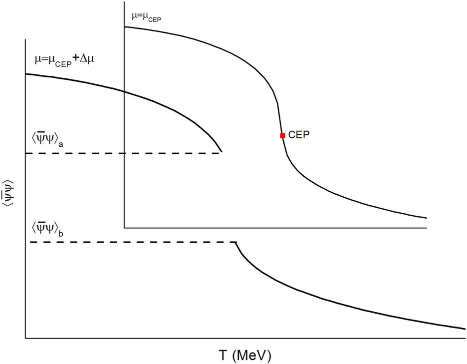When the chemical potential increases from μ _CEP to μ _CEP + Δμ, one should be able to measure a jump in the order parameter when going from lower to higher temperature values and from 〈 ψ ¯ ψ 〉 a to 〈 ψ ¯ ψ 〉 b , where 〈 ψ ¯ ψ 〉 a > 〈 ψ ¯ ψ 〉 b . The crossover zone will be regarded as the set of T, μ values where the chiral condensate is contained between 〈 ψ ¯ ψ 〉 a and 〈 ψ ¯ ψ 〉 b . The advantages this approach are that we mathematically ensure that the crossover zone ends at the CEP and also ensure that for every T, μ point contained in this zone both phases coexist, truly belonging to the crossover zone.

Figure 8

Condensate discontinuity criterion.

By applying this criterion, the crossover zone ends exactly at the CEP coordinates of T = 27 MeV, μ = 327 MeV for UV (A), T = 37 MeV, μ = 332 MeV for UV (B) and T = 29 MeV, μ = 298 MeV for IR. All this can be seen in Figure 9. The main disadvantages of this approach are the resolution dependency of this zone and the fact that the presence of a CEP is needed to define the crossover zone, when in reality a CEP does not need to exist for a crossover zone to exist.

Figure 9

Phase diagram for the condensate discontinuity criterion. (a) UV (A), m ₀ = 5 MeV, (b) UV (B), m ₀ = 5.5 MeV, (c) IR, m ₀ = 5 MeV.

5.5.2 Inflection point criterion

The other way to define a crossover zone that does not require the existence of a CEP involves the concept of the chiral susceptibility. Capitalizing on the fact that for any constant value of temperature or chemical potential at the crossover zone the chiral susceptibility is a bell-like curve, we can define the crossover zone as everything in between the two inflection points of the curve. This has the advantage that is not dependent on the resolution or the existence of a CEP. However, the crossover zone as defined by this is not assured to end at the CEP, if there is one. In this criterion, when a CEP exists (Figure 10a, b and d), the crossover region closes, and for higher chemical potentials, it continues as a single point. This continuation of the region can be interpreted as the location of the first-order phase transition, which coincides with the one displayed in Figure 7a, b and d. When there is no CEP (Figure 10c, e, f and g), the crossover region continues until the chemical potential axis without closing completely. In PTR (1) and UV (C), this region’s bulk is approximately the same throughout all chemical potential values (Figure 10e and c, respectively), and in PV and PTR (2) (Figure 10g and f), the crossover’s bulk diminishes for higher chemical potential values.

Figure 10

Phase diagram for the inflection point criterion. (a) UV (A), m ₀ = 5 MeV, (b) UV (B), m ₀ = 5.5 MeV, (c) UV (C), m ₀ = 3 MeV, (d) IR, m ₀ = 5 MeV, (e) PTR (1), m ₀ = 5 MeV, (f) PTR (2), m ₀ = 5 MeV, (g) PV, m ₀ = 5 MeV.

6 Discussion

For both phase transition criteria, in the PTR and PV schemes, where the momentum values are from zero to infinity, the phase transition curves are at higher values of temperature and chemical potential than the ones for UV and IR. Since we are considering unconfined quarks in the model, only chiral phase is being studied. When the UV scheme has larger values for finite current quark mass, the value of T _c turns out to be higher than the cases with lower current masses, but the PTR (1) case is still the highest. Interestingly, PTR (1) is the only scheme whose phase transition curve is unaffected by the phase transition criteria. We added the PTR (2) scheme explicitly because of this, as now we know that the change in the terms that are affected by the integration regulator also changes this immunity to the criteria.

The NJL model is very sensitive to the setting parameters [29], although with the differences in the m ₀ value we can notice that the regularization procedure (momentum range) has a bigger impact in the phase diagrams than the parameters used.

The fact that the IR scheme was that different to the UV scheme is quite surprising, given the fact that the IR cutoff was introduced in order to avoid certain phenomenon related to confinement, which is not naturally present in the NJL model, and the changes obtained here were only related to the chiral symmetry.

Regarding the crossover criteria, we notice that, in the cases where a CEP exists, both criteria yield crossover ranges that do not overlap, but both of them end in a single point at the CEP. One should not expect to see either an overlap between both criteria or the fact that both of them end at the CEP; if one criterion is heavily dependent on the condensate values whereas the other is dependent on the susceptibility behavior, the latter does not depend directly on the former.

The inflection point criterion continues as a single line which represents the first-order transition, which also acts as an inflection point to the chiral susceptibility. This does not happen on the condensate discontinuity criterion, where the crossover is highlighted by the set of condensate values between the jump discontinuity, which do not appear after the CEP. If there is no CEP, the position of both inflection points is well separated for all temperature and chemical potential values, which translates to a wide crossover region in the entirety of the diagram (Figures 10c, e, f and g).

The condensate discontinuity criterion can be regarded as an “extension” of the global phase transition criterion, where a condensate value was used as a threshold for the definition of one phase and another, whereas the crossover is defined by a set of values around that threshold. For this reason, the condensate discontinuity-defined crossovers (Figure 9) always contain the global criterion curves before reaching the CEP (Figure 7a, b and d).

On the other hand, the inflection point criterion relies heavily on the chiral susceptibility values around the phase transition and the crossover. The local criterion positions the transition curve in the local maxima of the chiral susceptibility. This transition curve is always contained between the two curves obtained by positioning the inflection points of the chiral susceptibility on the T–μ plane. Because of this, the inflection point criterion crossover sections (Figure 10) always contain the local phase transition curve, and they may or may not contain the global phase transition curves (Figure 7).

With this, it can be seen that the overlapping of both curves of the phase transition criteria must not be interpreted as the limit of the crossover range, but as two different ways to locate the points where the crossover is at its largest extent.

There have been some studies in the literature that use other regularization schemes. The dimensional regularization [28,29,63,64] uses an analytic continuation of the spacetime dimensions as the regulator parameter. Other regularization schemes include various types of form factors [63,65], a regularization scheme that turns off the coupling constant after a certain cutoff [66] and a regularization scheme that separates the vacuum and medium contributions to the non-convergent integrands dubbed the medium separation scheme [67]. Our work in the near future intends to use the criteria used in this article to study the behavior of the NJL phase diagram under all these regularization schemes. The NJL model, sensitive to the regularization procedures as it is, is bound to present many sorts of interesting behavior on the chiral phase diagrams with all these variables.

7 Conclusion

In this article, we studied the width of the crossover region on several regularization methods on the NJL model. Similar to the sensitivity of the CEP position to the regularization schemes and the setting parameters [29], we found that the crossover region is quite sensitive to these factors. This sensitivity also happens in other models like the linear sigma model [68], where the position of the CEP can drastically change its position with respect to the set pion mass and sigma mass, or in Schwinger–Dyson equations [69], where the position of the CEP is highly sensitive to the chiral chemical potential. Therefore, it is reasonable to assume that the crossover range is sensitive to these parameters in these models as well.

Inflection points, while being a criterion that is reliable to use because of the good behavior of the chiral susceptibility in every regularization method, do not reproduce the width of the crossover found on the condensate discontinuity criterion.

The fact that both the crossover criteria do not overlap for low chemical potential values makes it difficult to determine the starting point and ending point of the crossover. While mathematically the width is infinite, in reality, we distinguish one chiral phase from another by the total presence or total absence of chiral condensates, which is always bound to change due to quantum fluctuations.

rubenmorones@yahoo.com.mx

Acknowledgements

B. Mata and E. Valbuena acknowledge the scholarship support from Consejo Nacional de Ciencia y Tecnología (CONACyT).

References

[1] Cui Z-F, Hou F-Y, Shi Y-M, Wang Y-L, Zong H-S. Progress in vacuum susceptibilities and their applications to the chiral phase transition of QCD. Ann Phys. 2015;358(1):172–205.10.1016/j.aop.2015.03.025Search in Google Scholar

[2] Wilczek F. Origins of mass. Open Phys. 2012;10(5):1021–37.10.2478/s11534-012-0121-0Search in Google Scholar

[3] Ciminale M, Gatto R, Ippolito ND, Nardulli G, Ruggieri M. Three flavor Nambu–Jona-Lasinio model with Polyakov loop and competition with nuclear matter. Phys Rev D Part Fields Gravitation Cosmol. 2008;77(5):054023.10.1103/PhysRevD.77.054023Search in Google Scholar

[4] Fukushima K, Hatsuda T. The phase diagram of dense QCD. Rep Prog Phys. 2011;74(1):014001.10.1088/0034-4885/74/1/014001Search in Google Scholar

[5] Wetterich C. Connection between chiral symmetry restoration and deconfinement. Phys Rev D Part Fields. 2002;66(5):056003.10.1103/PhysRevD.66.056003Search in Google Scholar

[6] Reinhardt H, Weigel H. Vacuum nature of the QCD condensates. Phys Rev D Part Fields Gravitation Cosmol. 2012;85(7):074029.10.1103/PhysRevD.85.074029Search in Google Scholar

[7] Kapusta J, Lichard P, Seibert D. High-energy photons from quark–gluon plasma versus hot hadronic gas. Phys Rev D Part Fields. 1993;44(9):2774–88.10.1103/PhysRevD.44.2774Search in Google Scholar

[8] STAR Collaboration, Adams J. Experimental and theoretical challenges in the search for the quark–gluon plasma: the STAR Collaboration's critical assessment of the evidence from RHIC collisions. Nucl Phys A. 2005;757(1–2):102–83.10.1016/j.nuclphysa.2005.03.085Search in Google Scholar

[9] Martinez G. Advances in Quark Gluon Plasma. arXiv:1304.1452 [nucl-ex].Search in Google Scholar

[10] Meyer-Ortmanns H. Phase transitions in quantum chromodynamics. Rev Mod Phys. 1996;68(2):473–598.10.1103/RevModPhys.68.473Search in Google Scholar

[11] Hatsuda T, Kunihiro T. QCD phenomenology based on a chiral effective Lagrangian. Phys Rep. 1994;247(5–6):221–367.10.1016/0370-1573(94)90022-1Search in Google Scholar

[12] Klevansky SP. The Nambu–Jona-Lasinio model of quantum chromodynamics. Rev Mod Phys. 1992;64(3):649–708.10.1103/RevModPhys.64.649Search in Google Scholar

[13] Weise W. From QCD symmetries to nuclei and neutron stars. Int J Mod Phys E. 2018;27(12):1840004.10.1142/S0218301318400049Search in Google Scholar

[14] Lastowiecki R, Blaschke D, Fischer T, Klahn T. Quark matter in high-mass neutron stars? Phys Part Nucl. 2015;46(5):843–45.10.1134/S1063779615050159Search in Google Scholar

[15] Buballa M, Carignano S. Inhomogeneous chiral symmetry breaking in dense neutron-star matter. Eur Phys J A. 2016;52(3):1–6.10.1140/epja/i2016-16057-6Search in Google Scholar

[16] Lenzi CH, Schneider AS, Providência C, Marinho RM. Compact stars with a quark core within the Nambu–Jona-Lasinio (NJL) model. Phys Rev C Nucl Phys. 2010;82(1):015809.10.1103/PhysRevC.82.015809Search in Google Scholar

[17] Philipsen O. The QCD equation of state from the lattice. Prog Part Nucl Phys. 2013;70(1):55–107.10.1016/j.ppnp.2012.09.003Search in Google Scholar

[18] Kovacs EVE, Sinclair DK, Kogut JB. Return of the finite-temperature phase transition in the chiral limit of lattice QCD. Phys Rev Lett. 1987;58(8):751–4.10.1103/PhysRevLett.58.751Search in Google Scholar PubMed

[19] Engel GP, Giusti L, Lottini S, Sommer R. Chiral symmetry breaking in QCD with two light flavors. Phys Rev Lett. 2015;114(11):112001.10.1103/PhysRevLett.114.112001Search in Google Scholar PubMed

[20] Carlomagno JP, Gómez D, Scoccola NN. Inhomogeneous phases in nonlocal chiral quark models. Phys Rev D Part Fields Gravitation Cosmol. 2015;92(8):056007.10.1103/PhysRevD.92.056007Search in Google Scholar

[21] Bhattacharya T, Buchoff MI, Christ NH, Ding H-T, Gupta R, Jung C, et al. QCD phase transition with chiral quarks and physical quark masses. Phys Rev Lett. 2014;113(8):082001.10.1103/PhysRevLett.113.082001Search in Google Scholar PubMed

[22] Gavai RV, Gupta S. On the critical end point of QCD. Phys Rev D Part Fields Gravitation Cosmol. 2005;71(11):114014.10.1103/PhysRevD.71.114014Search in Google Scholar

[23] Ejiri S. Existence of the critical point in finite density lattice QCD. Phys Rev D Part Fields Gravitation Cosmol. 2008;77(1):014508.10.1103/PhysRevD.77.014508Search in Google Scholar

[24] Alford M, Rajagopal K, Wilczek F. QCD at finite baryon density: nucleon droplets and color superconductivity. Phys Lett B. 1998;422(1–4):247–56.10.1016/S0370-2693(98)00051-3Search in Google Scholar

[25] Costa P, Ruivo MC, de Sousa CA. Thermodynamics and critical behavior in the Nambu–Jona-Lasinio model of QCD. Phys Rev D Part Fields Gravitation Cosmol. 2008;77(9):096001.10.1103/PhysRevD.77.096001Search in Google Scholar

[26] Lu Y, Du Y-L, Cui Z-F, Zong H-S. Critical behaviors near the (tri-)critical end point of QCD within the NJL model. Eur Phys J C. 2015;75(10):1–7.10.1140/epjc/s10052-015-3720-2Search in Google Scholar

[27] Vogl U, Weise W. The Nambu and Jona-Lasinio model: its implications for Hadrons and nuclei. Prog Part Nucl Phys. 1991;27(1):195–272.10.1016/0146-6410(91)90005-9Search in Google Scholar

[28] Kohyama H, Kimura D, Inagaki T. Parameter fitting in three-flavor Nambu-Jona-Lasinio model with various regularizations. Nucl Phys B. 2016;906(1):524–48.10.1016/j.nuclphysb.2016.03.015Search in Google Scholar

[29] Kohyama H, Kimura D, Inagaki T. Regularization dependence on phase diagram in Nambu–Jona-Lasinio model. Nucl Phys B. 2015;896(1):682–715.10.1016/j.nuclphysb.2015.05.015Search in Google Scholar

[30] Costa P, Hansen H, Ruivo MC, Sousa CA. How parameters and regularization affect the Polyakov–Nambu–Jona-Lasinio model phase diagram and thermodynamic quantities. Phys Rev D Part Fields Gravitation Cosmol. 2010;81(1):016007.10.1103/PhysRevD.81.016007Search in Google Scholar

[31] Nambu Y, Jona-Lasinio G. Dynamical model of elementary particles based on an analogy with superconductivity I. Phys Rev. 1961;122(1):345–58.10.1103/PhysRev.122.345Search in Google Scholar

[32] Nambu Y, Jona-Lasinio G. Dynamical model of elementary particles based on an analogy with superconductivity II. Phys Rev. 1961;124(1):246–54.10.1103/PhysRev.124.246Search in Google Scholar

[33] Torres-Rincon JM, Aichelin J. Equation of state of a quark-meson mixture in the improved Polyakov–Nambu–Jona-Lasinio model at finite chemical potential. Phys Rev C. 2017;96(4):045206.10.1103/PhysRevC.96.045205Search in Google Scholar

[34] Whittenbury DL, Carrillo-Serrano ME, Thomas AW. Quark–meson coupling model based upon the Nambu–Jona Lasinio model. Phys Lett B. 2016;762(1):467–72.10.1016/j.physletb.2016.09.057Search in Google Scholar

[35] Yamazaki K, Matsui T. Quark–Hadron phase transition in a three flavor PNJL model for interacting quarks. Nucl Phys A. 2014;922(1):237–61.10.1016/j.nuclphysa.2013.12.010Search in Google Scholar

[36] Buballa M. NJL-model analysis of dense quark matter. Phys Rep. 2005;407(1):205.10.1016/j.physrep.2004.11.004Search in Google Scholar

[37] Volkov MK, Radzhabov AE. Forty-fifth anniversary of the Nambu-Jona-Lasinio model. arxiv:hep-ph/0508263.Search in Google Scholar

[38] Ohnishi A. Approaches to QCD phase diagram; effective models, strong-coupling lattice QCD, and compact stars. J Phys Conf Ser. 2016;668(1):012004.10.1088/1742-6596/668/1/012004Search in Google Scholar

[39] Le Bellac M. Dirac and gauge fields at finite temperature. Thermal Field Theory. Cambridge: Cambridge University Press; 1996. p. 86–113 (Cambridge Monographs on Mathematical Physics).10.1017/CBO9780511721700.006Search in Google Scholar

[40] Asakawa M, Yazaki K. Chiral restoration at finite density and temperature. Nucl Phys A. 1989;504(4):668–84.10.1016/0375-9474(89)90002-XSearch in Google Scholar

[41] Boyd G, Fingberg J, Karsch F, Kärkkäinen L, Petersson B. Critical exponents of the chiral transition in strong coupling QCD. Nucl Phys B. 1992;376(1):199–217.10.1016/0550-3213(92)90074-LSearch in Google Scholar

[42] Zhao Y, Chang L, Yuan W, Liu Y-X. Chiral susceptibility and chiral phase transition in Nambu–Jona-Lasinio model. Eur Phys J C. 2008;56(4):483–92.10.1140/epjc/s10052-008-0673-8Search in Google Scholar

[43] Morones-Ibarra JR, Enriquez-Perez-Gavilán A, Herández-Rodríguez AI, Flores-Baez FV, Mata-Carrizalez NB, Valbuena-Ordoñez E. Chiral symmetry restoration and the critical end point in QCD. Open Phys. 2017;15(1):1039–44.10.1515/phys-2017-0130Search in Google Scholar

[44] Fukushima K. Phase diagrams in the three-flavor Nambu–Jona-Lasinio model with the Polyakov loop. Phys Rev D Part Fields Gravitation Cosmol. 2008;77(11):114028.10.1103/PhysRevD.77.114028Search in Google Scholar

[45] Fukushima K, Sasaki C. The phase diagram of nuclear and quark matter at high baryon density. Prog Part Nucl Phys. 2013;72(1):99–154.10.1016/j.ppnp.2013.05.003Search in Google Scholar

[46] Ebert D, Feldmann T, Reinhardt H. Extended NJL model for light and heavy mesons without q–q thresholds. Phys Lett B. 1996;388(1):154–60.10.1016/0370-2693(96)01158-6Search in Google Scholar

[47] Blaschke D, Burau G, Volkov MK, Yudichev VL. NJL model with infrared confinement. arXiv:hep-ph/9812503.Search in Google Scholar

[48] Blaschke DB, Burau GRG, Volkov MK. Chiral quark model with infrared cut-off for the description of meson properties in hot matter. Eur Phys J A. 2001;11(3):319–27.10.1007/PL00022984Search in Google Scholar

[49] Dubinin A, Blaschke D, Kalinovsky YL. Pion and sigma meson dissociation in a modified NJL model at finite temperature. Acta Phys Polon Supp. 2014;7(1):215–23.10.5506/APhysPolBSupp.7.215Search in Google Scholar

[50] Zhang J-L, Shi Y-M, Xu S-S, Zong H-S. Proper time regularization at finite quark chemical potential. Mod Phys Lett A. 2016;31(14):1650086.10.1142/S0217732316500863Search in Google Scholar

[51] Pauli W, Villars F. On the invariant regularization in relativistic quantum theory. Rev Mod Phys. 1949;21(3):434–44.10.1103/RevModPhys.21.434Search in Google Scholar

[52] Mao S. Inverse magnetic catalysis in Nambu–Jona-Lasinio model beyond mean field. Phys Lett B. 2016;758(1):195–9.10.1016/j.physletb.2016.05.018Search in Google Scholar

[53] Kalinovsky YL, Friesen AV. Properties of mesons and critical points in the Nambu–Jona-Lasinio model with different regularizations. Phys Elem Part Atom Nucl. 2015;12(6):737–43.10.1134/S1547477115060060Search in Google Scholar

[54] Kahana D, Lavelle M. On the Pauli–Villars regularisation scheme in the NJL model. Phys Lett B. 1993;298(3–4):397–99.10.1016/0370-2693(93)91839-FSearch in Google Scholar

[55] Ratti C, Thaler MA, Weise W. Phases of QCD: lattice thermodynamics and a field theoretical model. Phys Rev D Part Fields Gravitation Cosmol. 2006;73(1):014019.10.1103/PhysRevD.73.014019Search in Google Scholar

[56] Cui Z-F, Zhang J-L, Zong H-S. Proper time regularization and the QCD chiral phase transition. Sci Rep. 2017;7(1):45937.10.1038/srep45937Search in Google Scholar PubMed PubMed Central

[57] Morones JR, Garza AJ, Flores FV. Thermodynamic properties of light mesons and phase transition in an extended SU(2) NJL model. Mod Phys Lett A. 2019;34(13):1950070.10.1142/S0217732319500706Search in Google Scholar

[58] Yuan W, Chen H, Liu Y-X. Dyson–Schwinger equation and quantum phase transitions in massless QCD. Phys Lett B. 2006;637(1):69–74.10.1016/j.physletb.2006.03.076Search in Google Scholar

[59] Sasaki C, Friman B, Redlich K. Susceptibilities and the phase structure of a chiral model with Polyakov loops. Phys Rev D Part Fields Gravitation Cosmol. 2007;75(7):074013.10.1103/PhysRevD.75.074013Search in Google Scholar

[60] Du Y-I, Cui Z-F, Xia Y-H, Zong H-S. Discussions on the crossover property within the Nambu–Jona-Lasinio model. Phys Rev D Part Fields Gravitation Cosmol. 2013;88(11):114019.10.1103/PhysRevD.88.114019Search in Google Scholar

[61] Moreira J, Hiller B, Osipov AA, Blin AH. Thermodynamic potential with correct asymptotics for PNJL model. Int J Mod Phys A. 2012;27(11):1250060.10.1142/S0217751X12500601Search in Google Scholar

[62] Fodor Z, Katz SD. Lattice determination of the critical point of QCD at finite T and μ. JHEP. 2002;2002(3):014.10.1088/1126-6708/2002/03/014Search in Google Scholar

[63] Andersen JO, Naylor WR, Tranberg A. Phase diagram of QCD in a magnetic field. Rev Mod Phys. 2016;88(2):025001.10.1103/RevModPhys.88.025001Search in Google Scholar

[64] Fujihara T, Kimura D, Inagaki T, Kvinikhidze A. High density quark matter in the NJL model with dimensional vs. cut-off regularization. Phys Rev D Part Fields Gravitation Cosmol. 2009;79(9):096008.10.1103/PhysRevD.79.096008Search in Google Scholar

[65] Duarte DC, Allen PG, Farias RLS, Manso PHA, Ramos RO, Scoccola NN. BEC-BCS crossover in a cold and magnetized two color NJL model. Phys Rev D. 2016;93(2):025017.10.1103/PhysRevD.93.025017Search in Google Scholar

[66] Bratovic N, Hatsuda T, Weise W. Role of vector interaction and axial anomaly in the PNJL modeling of the QCD phase diagram. Phys Lett B. 2013;719(1):131–5.10.1016/j.physletb.2013.01.003Search in Google Scholar

[67] Farias RLS, Duarte DC, Krein G, Ramos RO. Thermodynamics of quark matter with a chiral imbalance. Phys Rev D. 2016;94(7):074011.10.1103/PhysRevD.94.074011Search in Google Scholar

[68] Schaefer B-J, Wagner M. On the QCD phase structure from effective models. Prog Part Nucl Phys. 2009;62(2):381–5.10.1016/j.ppnp.2008.12.009Search in Google Scholar

[69] Wang B, Wang Y-L, Cui Z-F, Zong H-S. Effect of the chiral chemical potential on the position of the critical endpoint. Phys Rev D Part Fields Gravitation Cosmol. 2015;91(3):034017.10.1103/PhysRevD.91.034017Search in Google Scholar

Received: 2019-09-18

Revised: 2020-03-02

Accepted: 2020-03-03

Published Online: 2020-05-20

This work is licensed under the Creative Commons Attribution 4.0 International License.

Articles in the same Issue

https://doi.org/10.1515/phys-2020-0010

Keywords for this article

Nambu–Jona-Lasinio model; chiral phase transition; critical end point; chiral symmetry restoration; chiral susceptibility; QCD effective theories

Creative Commons

BY 4.0