Closed-form wave structures of the space-time fractional Hirota–Satsuma coupled KdV equation with nonlinear physical phenomena
-
 ,
and
,
and

Abstract
The present paper applies the variation of
1 Introduction
Nonlinear dynamical systems play an important role in physics. New ideas in physics including astrophysics, computational physics, fluid dynamic, mathematical physics, biological physics and medical physics often explain the fundamental mechanisms studied by other sciences and suggest new avenues of research in academic disciplines such as mathematics. Nature and research problems and most of the life and compound phenomena are explained and invented through fractional wave models. For example, the fluid-dynamic traffic model [1] could succeed the deficiency based upon the hypothesis of continuum traffic flow, the principles of fractional calculus could model the dynamical methods in fluids and porous structures [2] and fractional derivatives can form the nonlinear oscillation of earthquake [3]. For all the attention, it is an indispensable task to attain the closed-form wave structures of the fractional differential equations (FDEs). Various meaningful and truthful approaches have been interpolated for achieving the closed-form wave structures of FDEs, including the
Here, we introduce a new method [31] for nonlinear FDEs based on the homogenous balancing method employing wave transformation. In this research, through the transformation
2 Preliminaries
Herein, we acquaint a few definitions, characters, properties, theorems and fundamental facts, which are implemented throughout this article.
2.1 The modified Riemann–Liouville derivative
Fractional calculus possesses several ways to generalize the concept of differential derivatives to fractional derivatives [51,52].
Definition 2.1
A real function
Definition 2.2
Suppose that
in which
or
and
Definition 2.3
The Mittag–Leffler function including two parameters is represented as follows [54]
Some notable characteristics for the fractional derivative are as follows:
2.2 The fractional complex transformation
This section performs the complex fractional transformation for the fractional-order ordinary differential equation (ODE). First, we explore the nonlinear fractional ODE:
where
We investigate equation (6) through the transformation
3 Glimpse of the method
At this moment, the general scheme of the variation of
Step 1: Calculate N through rule of the homogeneous balance in equation (7).
Step 2: Considering the method can be expressed as the form:
(8)where
(9)(10)These coupled Riccati equations give us four types of hyperbolic function solutions including sech, tanh, csch and coth such as
(11)(12)Step 3: A polynomial in L or N is accomplished plugging equation (8) into equation (7). Determining the coefficients of the equivalent power of L or N produces a system of algebraic equations, which can be determined to construct the values of
4 Implementation of the method
To illustrate the idea of the new method, we implement the process on the space-time fractional Hirota–Satsuma coupled KdV equation. We implement the new method to the considered model, which models the intercommunication between two long waves that have well-defined dispersion connection:
where
where
Applying the homogeneous balance rule on equation (14) yields
where
Case 1: Let
(16)(17)(18)(19)(20)(21)Case 2: Let
(22)(23)(24)(25)(26)(27)Case 3: Let
(28)(29)(30)(31)(32)(33)Case 4: Let
(34)(35)(36)(37)(38)(39)Case 5: Let
A picture is an indispensable tool for conversation and to demonstrate the results to the difficulties lucidly. When performing the computation in daily life, we require the fundamental understanding of constructing the use of pictures. Therefore, the graphical presentations of few obtained results are depicted in Figures 1–6.

The picture of the result in

The picture of the result in

The picture of the result in

The picture of the result in
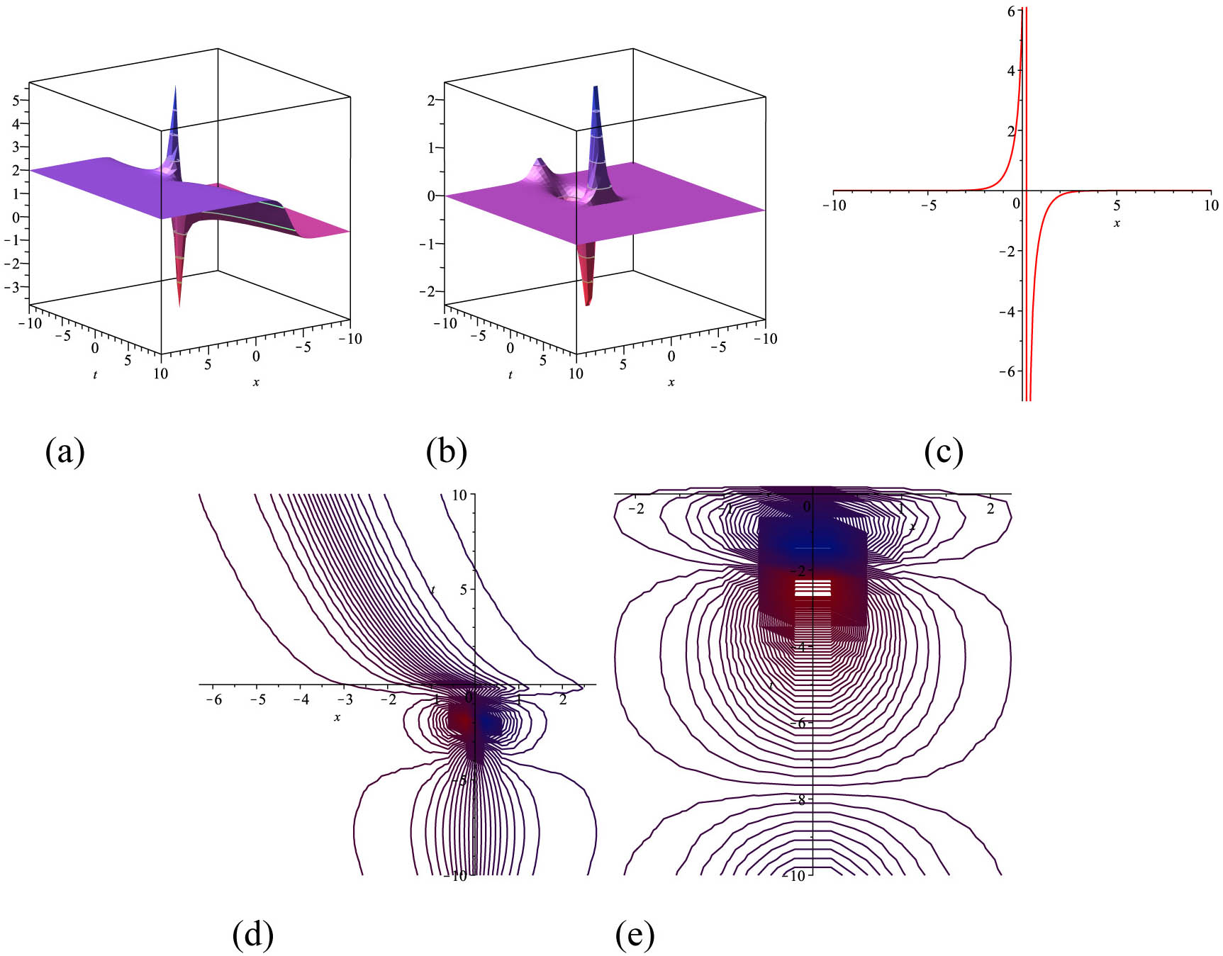
The picture of the result in

The picture of the result in
5 Discussions and future work
In this research, the suggested method has been triumphantly displayed to attain new closed-form wave solutions of equation (13). It has been determined that the complex fractional transformation and the advanced method are an essential and significant mathematical device in analyzing closed-form wave structures of a whole class of fractional FDEs. Consequently, a few new closed-form wave answers of the equation are determined.
The compensations and legality of the recommended approach over the extended Kudryashov approach are as follows. The critical compensation of the proposed method over the extended Kudryashov approach is that the proposed method implements numerous general and plentiful new closed-form wave structures. The closed-form wave solutions of nonlinear FDE have its vital importance to show the complicated physical aspects. For example, [36] extends the Kudryashov method to solve equation
Acknowledgements
The authors would like to acknowledge CAS-TWAS president’s fellowship program. The author thanks the referees for their suggestions and comments.
-
Competing interests: This research received no specific grant from any funding agency in the public, commercial or not-for-profit sectors. The authors did not have any competing interests in this research.
-
Author contributions: All parts contained in the research carried out by the authors through hard work and a review of the various references and contributions in the field of mathematics and Applied physics.
-
Availability of data and materials: Data sharing is not applicable to this article as no datasets were generated or analyzed during the current study.
-
Funding: No funding for this article.
References
[1] Podlubny I . Fractional Differential Equations. New York: Academic Press; 1999.Search in Google Scholar
[2] Miller KS , Ross B . An Introduction to the Fractional Calculus and Fractional Differential Equations. New York: John Wiley; 1993.Search in Google Scholar
[3] Mainardi F . Fractional Calculus Some Basic Problems in Continum and Statistical Mechanics. New York: Springer-Verlag; 1997.10.1007/978-3-7091-2664-6Search in Google Scholar
[4] Alam M , Belgacem F . Microtubules nonlinear models dynamics investigations through the exp(−ϕ(ξ))-expansion method implementation. Mathematics. 2016;4:6.10.3390/math4010006Search in Google Scholar
[5] Alam M , Tunc C . An analytical method for solving exact solutions of the nonlinear bogoyavlenskii equation and the nonlinear diffusive predator-prey system. Alex Eng J. 2016;55:1855–65.10.1016/j.aej.2016.04.024Search in Google Scholar
[6] Sonmezoglu A . Exact solutions for some fractional differential equations. Adv Math Phys. 2015;2015:567842 10.1155/2015/567842Search in Google Scholar
[7] Karaagac B . New exact solutions for some fractional order differential equations via improved sub-equation method. Discret Cont Dyn Syst – S. 2019;12:447–54.10.3934/dcdss.2019029Search in Google Scholar
[8] Iqbal M , Seadawy AR , Lu D . Construction of solitary wave solutions to the nonlinear modified Kortewege-de Vries dynamical equation in unmagnetized plasma via mathematical methods. Mod Phys Lett A. 2018;33(32):1850183.10.1142/S0217732318501833Search in Google Scholar
[9] Martineza HY , Aguilarb JFG , Baleanu D . Beta-derivative and sub-equation method applied to the optical solitons in medium with parabolic law nonlinearity and higher order dispersion. Optik. 2018;155:357–65.10.1016/j.ijleo.2017.10.104Search in Google Scholar
[10] Saleh R , Kassem M , Mabrouk SM . Exact solutions of nonlinear fractional order partial differential equations via singular manifold method. Chin J Phys. 2019;61:290–300.10.1016/j.cjph.2019.09.005Search in Google Scholar
[11] Delgado VFM , Aguilar JFG , Torres L , Jimenez RFE , Hernandez MAT . Exact solutions for the liénard type model via fractional homotopy methods. Fract Derivatives Mittag–Leffler Kernel. 2019;194:269–91.10.1007/978-3-030-11662-0_16Search in Google Scholar
[12] Abuasad S , Moaddy K , Hashim I . Analytical treatment of two-dimensional fractional helmholtz equations. J King Saud Univ – Sci. 2019;31:659–66.10.1016/j.jksus.2018.02.002Search in Google Scholar
[13] Alam MN , Tunc C . Constructions of the optical solitons and others soliton to the conformable fractional zakharov–kuznetsov equation with power law nonlinearity. J Taibah Univ Med Sci. 2020;15:263–72. 10.1080/16583655.2019.1708542.Search in Google Scholar
[14] Seadawy AR . Three-dimensional weakly nonlinear shallow water waves regime and its travelling wave solutions. Int J Comput Methods. 2018;15:1850017.10.1142/S0219876218500172Search in Google Scholar
[15] Kadkhoda N , Jafari H . An analytical approach to obtain exact solutions of some space-time conformable fractional differential equations. Adv Differ Equ. 2019;2019;428.10.1186/s13662-019-2349-0Search in Google Scholar
[16] Seadawy AR , Manafian J . New soliton solution to the longitudinal wave equation in a magneto-electro-elastic circular rod. Results Phys. 2018;8:1158–67.10.1016/j.rinp.2018.01.062Search in Google Scholar
[17] Lu D , Seadawy AR , Ali A . Dispersive traveling wave solutions of the equal-width and modified equal-width equations via mathematical methods and its applications. Results Phys. 2018;9:313–20.10.1016/j.rinp.2018.02.036Search in Google Scholar
[18] Helal MA , Seadawy AR , Zekry MH . Stability analysis of solitary wave solutions for the fourth-order nonlinear Boussinesq water wave equation. Appl Math Comput. 2014;232:1094–103.10.1016/j.amc.2014.01.066Search in Google Scholar
[19] Shi D , Zhang Y . Diversity of exact solutions to the conformable space-time fractional mew equation. Appl Math Lett. 2020;99:105994.10.1016/j.aml.2019.07.025Search in Google Scholar
[20] Seadawy AR , El-Rashidy K . Dispersive solitary wave solutions of kadomtsev–petviashivili and modified kadomtsev–petviashivili dynamical equations in unmagnetized dust plasma. Results Phys. 2018;8:1216–22.10.1016/j.rinp.2018.01.053Search in Google Scholar
[21] Lu D , Seadawy AR , Ali A . Applications of exact traveling wave solutions of modified Liouville and the symmetric regularized long wave equations via two new techniques. Results Phys. 2018;9:1403–10.10.1016/j.rinp.2018.04.039Search in Google Scholar
[22] Arshad M , Seadawy A , Lu D . Elliptic function and solitary wave solutions of the higher-order nonlinear Schrodinger dynamical equation with fourth-order dispersion and cubic-quintic nonlinearity and its stability. Eur Phys J Plus. 2017;132:371.10.1140/epjp/i2017-11655-9Search in Google Scholar
[23] Zuriqat M . Exact solution for the fractional partial differential equation by homo separation analysis method. Afr Matematika. 2019;30:1133–43.10.1007/s13370-019-00707-xSearch in Google Scholar
[24] Arnous AH , Seadawy AR , Alqahtani RT , Biswas A . Optical solitons with complex ginzburg-landau equation by modified simple equation method. Opt – Int J Light Electron Opt. 2017;144:475–80.10.1016/j.ijleo.2017.07.013Search in Google Scholar
[25] Owyed S , Abdou MA , Abdel-Atyb AH , Nekhili WAR . Numerical and approximate solutions for coupled time fractional nonlinear evolutions equations via reduced differential transform method. Chaos, Solitons Fractals. 2019;217:109474.10.1016/j.chaos.2019.109474Search in Google Scholar
[26] Abdullah , Seadawy AR , Wang J . Mathematical methods and solitary wave solutions of three-dimensional zakharov–kuznetsov–burgers equation in dusty plasma and its applications. Results Phys. 2017;7:4269–77.10.1016/j.rinp.2017.10.045Search in Google Scholar
[27] Cenesiz Y , Tasbozan O , Kurt A . Functional variable method for conformable fractional modified kdv-zkequation and maccari system. Tbilisi Math J. 2017;10:117–25.10.1515/tmj-2017-0010Search in Google Scholar
[28] Seadawy AR , Lu D , Yue C . Travelling wave solutions of the generalized nonlinear fifth-order kdv water wave equations and its stability. J Taibah Univ Sci. 2017;11:623–33.10.1016/j.jtusci.2016.06.002Search in Google Scholar
[29] Sheikholeslami M . Cuo-water nanofluid free convection in a porous cavity considering darcy law. Eur Phys J Plus. 2017;132:132.10.1140/epjp/i2017-11330-3Search in Google Scholar
[30] Khater AH , Callebaut DK , Seadawy AR . General soliton solutions for nonlinear dispersive waves in convective type instabilities. Phys Scr. 2006;74:384–93.10.1088/0031-8949/74/3/015Search in Google Scholar
[31] Shehata AR , Abu-Amra SSM . Geometrical properties and exact solutions of three (3 + 1) -dimensional nonlinear evolution equations in mathematical physics using different expansion methods. J Adv Math Comput Sci. 2019;33:1–19.10.9734/jamcs/2019/v32i430149Search in Google Scholar
[32] Unal E , Gokdogan A . Solution of conformable fractional ordinary differential equations via differential transform method. Opt – Int J Light Electron Opt. 2017;128:264–73.10.1016/j.ijleo.2016.10.031Search in Google Scholar
[33] Alam MN , Li X . Exact traveling wave solutions to higher order nonlinear equations. J Ocean Eng Sci. 2019;4:276–88.10.1016/j.joes.2019.05.003Search in Google Scholar
[34] Arshad M , Seadawy A , Lu D . Modulation stability and optical soliton solutions of nonlinear Schrodinger equation with higher order dispersion and nonlinear terms and its applications. Superlattices Microstructures. 2017;112:422–34.10.1016/j.spmi.2017.09.054Search in Google Scholar
[35] Eslami M . Exact traveling wave solutions to the fractional coupled nonlinear schrodinger equations. Appl Math Comput. 2016;285:141–8.10.1016/j.amc.2016.03.032Search in Google Scholar
[36] Ege S , Misirli E . A new method for solving nonlinear fractional differential equations. N Trends Math Sci. 2017;5:225–33.10.20852/ntmsci.2017.141Search in Google Scholar
[37] Wazwaz A . Exact solutions with solitons and periodic structures for the zakharov–kuznetsov equation and its modified form. Commun Nonlinear Sci Numer Simul. 2005;10:597–606.10.1016/j.cnsns.2004.03.001Search in Google Scholar
[38] Akbulut MKA , Bekir A . Auxiliary equation method for fractional differential equations with modified riemann–liouville derivative. Int J Nonlin Sci Num. 2016;17:413–20.10.1515/ijnsns-2016-0023Search in Google Scholar
[39] Aly Seadawy , El-Rashidy K . Dispersive solitary wave solutions of Kadomtsev–Petviashivili and modified Kadomtsev–Petviashivili dynamical equations in unmagnetized dust plasma. Results Phys. 2018;8:1216–22.10.1016/j.rinp.2018.01.053Search in Google Scholar
[40] Kumar S , Kumar R , Singh J , Nisar KS , Kumard D . An efficient numerical scheme for fractional model of HIV-1 infection of CD4 + T-cells with the effect of antiviral drug therapy. Alex Eng J. 2020;216:634–42. 10.1016/j.aej.2019.12.046 Search in Google Scholar
[41] Kumar S , Kumar A , Momani S , Aldhaifallah M , Nisar KS . Numerical solutions of nonlinear fractional model arising in the appearance of the stripe patterns in two-dimensional systems. Adv Differ Equ. 2019;2019(1):413.10.1186/s13662-019-2334-7Search in Google Scholar
[42] Kumar S , Kumar A , Abbas S , Qurashi MA , Baleanu D . A modified analytical approach with existence and uniqueness for fractional Cauchy reaction-diffusion equations. Adv Differ Equ. 2020;2020(1):1–8.10.1186/s13662-019-2488-3Search in Google Scholar
[43] Sharma B , Kumar S , Cattani C , Baleanu D . Nonlinear dynamics of Cattaneo–Christov heat flux model for third-grade power-law fluid. J Comput Nonlinear Dyn. 2020 Jan 1;15(1):927–41.10.1115/1.4045406Search in Google Scholar
[44] Kumar S , Ghosh S , Samet B , Goufo EFD . An analysis for heat equations arises in diffusion process using new Yang–AbdelAty–Cattani fractional operator. Math Methods Appl Sci. 2020;162:572–84.Search in Google Scholar
[45] Tassaddiq A , Khan I , Nisar KS . Heat transfer analysis in sodium alginate based nanofluid using MoS2 nanoparticles: Atangana–Baleanu fractional model. Chaos, Solitons Fractals. 2020;130:109445.10.1016/j.chaos.2019.109445Search in Google Scholar
[46] Gao W , Senel M , Yel G , Baskonus HM , Senel B . New complex wave patterns to the electrical transmission line model arising in network system. Aims Math. 2020;5(3):1881–92.10.3934/math.2020125Search in Google Scholar
[47] Gao W , Ismael HF , Husien AM , Bulut H , Baskonus HM . Optical soliton solutions of the nonlinear Schrödinger and resonant nonlinear Schrödinger equation with Parabolic law. Appl Sci. 2020;10(1):219 , 1–20.10.3390/app10010219Search in Google Scholar
[48] Gao W , Yel G , Baskonus HM , Cattani C . Complex solitons in the conformable (2 + 1)-dimensional Ablowitz–Kaup–Newell–Segur equation. Aims Math. 2020;5(1):507–21.10.3934/math.2020034Search in Google Scholar
[49] Gao W , Rezazadeh H , Pinar Z , Baskonus HM , Sarwar S , Yel G . Novel explicit solutions for the nonlinear zoomeron equation by using newly extended direct algebraic technique. Opt Quant Electron. 2020;52(52):1–13.10.1007/s11082-019-2162-8Search in Google Scholar
[50] Cordero A , Jaiswal JP , Torregrosa JR . Stability analysis of fourth-order iterative method for finding multiple roots of non-linear equations. Appl Math Nonlinear Sci. 2019;4(1):43–56.10.2478/AMNS.2019.1.00005Search in Google Scholar
[51] Jumarie G . Table of some basic fractional calculus formulae derived from a modified riemann–liouville derivative for non-differentiable functions. Appl Math Lett. 2009;22:378–85.10.1016/j.aml.2008.06.003Search in Google Scholar
[52] Guner O . Singular and non-topological soliton solutions for nonlinear fractional differential equations. Chin Phys B. 2015;24:100201.10.1088/1674-1056/24/10/100201Search in Google Scholar
[53] Hartley T , Lorenzo C . Dynamics and control of initialized fractional-order systems. Nonlinear Dyn. 2002;29:201–33.10.1023/A:1016534921583Search in Google Scholar
[54] Kilbas A , Srivastava H , Trujillo J . Theory and applications of fractional differential equations. Amsterdam: Elsevier; 2006.Search in Google Scholar
© 2020 Md Nur Alam et al., published by De Gruyter
This work is licensed under the Creative Commons Attribution 4.0 International License.
Articles in the same Issue
- Regular Articles
- Model of electric charge distribution in the trap of a close-contact TENG system
- Dynamics of Online Collective Attention as Hawkes Self-exciting Process
- Enhanced Entanglement in Hybrid Cavity Mediated by a Two-way Coupled Quantum Dot
- The nonlinear integro-differential Ito dynamical equation via three modified mathematical methods and its analytical solutions
- Diagnostic model of low visibility events based on C4.5 algorithm
- Electronic temperature characteristics of laser-induced Fe plasma in fruits
- Comparative study of heat transfer enhancement on liquid-vapor separation plate condenser
- Characterization of the effects of a plasma injector driven by AC dielectric barrier discharge on ethylene-air diffusion flame structure
- Impact of double-diffusive convection and motile gyrotactic microorganisms on magnetohydrodynamics bioconvection tangent hyperbolic nanofluid
- Dependence of the crossover zone on the regularization method in the two-flavor Nambu–Jona-Lasinio model
- Novel numerical analysis for nonlinear advection–reaction–diffusion systems
- Heuristic decision of planned shop visit products based on similar reasoning method: From the perspective of organizational quality-specific immune
- Two-dimensional flow field distribution characteristics of flocking drainage pipes in tunnel
- Dynamic triaxial constitutive model for rock subjected to initial stress
- Automatic target recognition method for multitemporal remote sensing image
- Gaussons: optical solitons with log-law nonlinearity by Laplace–Adomian decomposition method
- Adaptive magnetic suspension anti-rolling device based on frequency modulation
- Dynamic response characteristics of 93W alloy with a spherical structure
- The heuristic model of energy propagation in free space, based on the detection of a current induced in a conductor inside a continuously covered conducting enclosure by an external radio frequency source
- Microchannel filter for air purification
- An explicit representation for the axisymmetric solutions of the free Maxwell equations
- Floquet analysis of linear dynamic RLC circuits
- Subpixel matching method for remote sensing image of ground features based on geographic information
- K-band luminosity–density relation at fixed parameters or for different galaxy families
- Effect of forward expansion angle on film cooling characteristics of shaped holes
- Analysis of the overvoltage cooperative control strategy for the small hydropower distribution network
- Stable walking of biped robot based on center of mass trajectory control
- Modeling and simulation of dynamic recrystallization behavior for Q890 steel plate based on plane strain compression tests
- Edge effect of multi-degree-of-freedom oscillatory actuator driven by vector control
- The effect of guide vane type on performance of multistage energy recovery hydraulic turbine (MERHT)
- Development of a generic framework for lumped parameter modeling
- Optimal control for generating excited state expansion in ring potential
- The phase inversion mechanism of the pH-sensitive reversible invert emulsion from w/o to o/w
- 3D bending simulation and mechanical properties of the OLED bending area
- Resonance overvoltage control algorithms in long cable frequency conversion drive based on discrete mathematics
- The measure of irregularities of nanosheets
- The predicted load balancing algorithm based on the dynamic exponential smoothing
- Influence of different seismic motion input modes on the performance of isolated structures with different seismic measures
- A comparative study of cohesive zone models for predicting delamination fracture behaviors of arterial wall
- Analysis on dynamic feature of cross arm light weighting for photovoltaic panel cleaning device in power station based on power correlation
- Some probability effects in the classical context
- Thermosoluted Marangoni convective flow towards a permeable Riga surface
- Simultaneous measurement of ionizing radiation and heart rate using a smartphone camera
- On the relations between some well-known methods and the projective Riccati equations
- Application of energy dissipation and damping structure in the reinforcement of shear wall in concrete engineering
- On-line detection algorithm of ore grade change in grinding grading system
- Testing algorithm for heat transfer performance of nanofluid-filled heat pipe based on neural network
- New optical solitons of conformable resonant nonlinear Schrödinger’s equation
- Numerical investigations of a new singular second-order nonlinear coupled functional Lane–Emden model
- Circularly symmetric algorithm for UWB RF signal receiving channel based on noise cancellation
- CH4 dissociation on the Pd/Cu(111) surface alloy: A DFT study
- On some novel exact solutions to the time fractional (2 + 1) dimensional Konopelchenko–Dubrovsky system arising in physical science
- An optimal system of group-invariant solutions and conserved quantities of a nonlinear fifth-order integrable equation
- Mining reasonable distance of horizontal concave slope based on variable scale chaotic algorithms
- Mathematical models for information classification and recognition of multi-target optical remote sensing images
- Hopkinson rod test results and constitutive description of TRIP780 steel resistance spot welding material
- Computational exploration for radiative flow of Sutterby nanofluid with variable temperature-dependent thermal conductivity and diffusion coefficient
- Analytical solution of one-dimensional Pennes’ bioheat equation
- MHD squeezed Darcy–Forchheimer nanofluid flow between two h–distance apart horizontal plates
- Analysis of irregularity measures of zigzag, rhombic, and honeycomb benzenoid systems
- A clustering algorithm based on nonuniform partition for WSNs
- An extension of Gronwall inequality in the theory of bodies with voids
- Rheological properties of oil–water Pickering emulsion stabilized by Fe3O4 solid nanoparticles
- Review Article
- Sine Topp-Leone-G family of distributions: Theory and applications
- Review of research, development and application of photovoltaic/thermal water systems
- Special Issue on Fundamental Physics of Thermal Transports and Energy Conversions
- Numerical analysis of sulfur dioxide absorption in water droplets
- Special Issue on Transport phenomena and thermal analysis in micro/nano-scale structure surfaces - Part I
- Random pore structure and REV scale flow analysis of engine particulate filter based on LBM
- Prediction of capillary suction in porous media based on micro-CT technology and B–C model
- Energy equilibrium analysis in the effervescent atomization
- Experimental investigation on steam/nitrogen condensation characteristics inside horizontal enhanced condensation channels
- Experimental analysis and ANN prediction on performances of finned oval-tube heat exchanger under different air inlet angles with limited experimental data
- Investigation on thermal-hydraulic performance prediction of a new parallel-flow shell and tube heat exchanger with different surrogate models
- Comparative study of the thermal performance of four different parallel flow shell and tube heat exchangers with different performance indicators
- Optimization of SCR inflow uniformity based on CFD simulation
- Kinetics and thermodynamics of SO2 adsorption on metal-loaded multiwalled carbon nanotubes
- Effect of the inner-surface baffles on the tangential acoustic mode in the cylindrical combustor
- Special Issue on Future challenges of advanced computational modeling on nonlinear physical phenomena - Part I
- Conserved vectors with conformable derivative for certain systems of partial differential equations with physical applications
- Some new extensions for fractional integral operator having exponential in the kernel and their applications in physical systems
- Exact optical solitons of the perturbed nonlinear Schrödinger–Hirota equation with Kerr law nonlinearity in nonlinear fiber optics
- Analytical mathematical schemes: Circular rod grounded via transverse Poisson’s effect and extensive wave propagation on the surface of water
- Closed-form wave structures of the space-time fractional Hirota–Satsuma coupled KdV equation with nonlinear physical phenomena
- Some misinterpretations and lack of understanding in differential operators with no singular kernels
- Stable solutions to the nonlinear RLC transmission line equation and the Sinh–Poisson equation arising in mathematical physics
- Calculation of focal values for first-order non-autonomous equation with algebraic and trigonometric coefficients
- Influence of interfacial electrokinetic on MHD radiative nanofluid flow in a permeable microchannel with Brownian motion and thermophoresis effects
- Standard routine techniques of modeling of tick-borne encephalitis
- Fractional residual power series method for the analytical and approximate studies of fractional physical phenomena
- Exact solutions of space–time fractional KdV–MKdV equation and Konopelchenko–Dubrovsky equation
- Approximate analytical fractional view of convection–diffusion equations
- Heat and mass transport investigation in radiative and chemically reacting fluid over a differentially heated surface and internal heating
- On solitary wave solutions of a peptide group system with higher order saturable nonlinearity
- Extension of optimal homotopy asymptotic method with use of Daftardar–Jeffery polynomials to Hirota–Satsuma coupled system of Korteweg–de Vries equations
- Unsteady nano-bioconvective channel flow with effect of nth order chemical reaction
- On the flow of MHD generalized maxwell fluid via porous rectangular duct
- Study on the applications of two analytical methods for the construction of traveling wave solutions of the modified equal width equation
- Numerical solution of two-term time-fractional PDE models arising in mathematical physics using local meshless method
- A powerful numerical technique for treating twelfth-order boundary value problems
- Fundamental solutions for the long–short-wave interaction system
- Role of fractal-fractional operators in modeling of rubella epidemic with optimized orders
- Exact solutions of the Laplace fractional boundary value problems via natural decomposition method
- Special Issue on 19th International Symposium on Electromagnetic Fields in Mechatronics, Electrical and Electronic Engineering
- Joint use of eddy current imaging and fuzzy similarities to assess the integrity of steel plates
- Uncertainty quantification in the design of wireless power transfer systems
- Influence of unequal stator tooth width on the performance of outer-rotor permanent magnet machines
- New elements within finite element modeling of magnetostriction phenomenon in BLDC motor
- Evaluation of localized heat transfer coefficient for induction heating apparatus by thermal fluid analysis based on the HSMAC method
- Experimental set up for magnetomechanical measurements with a closed flux path sample
- Influence of the earth connections of the PWM drive on the voltage constraints endured by the motor insulation
- High temperature machine: Characterization of materials for the electrical insulation
- Architecture choices for high-temperature synchronous machines
- Analytical study of air-gap surface force – application to electrical machines
- High-power density induction machines with increased windings temperature
- Influence of modern magnetic and insulation materials on dimensions and losses of large induction machines
- New emotional model environment for navigation in a virtual reality
- Performance comparison of axial-flux switched reluctance machines with non-oriented and grain-oriented electrical steel rotors
- Erratum
- Erratum to “Conserved vectors with conformable derivative for certain systems of partial differential equations with physical applications”