Random pore structure and REV scale flow analysis of engine particulate filter based on LBM

Chunrui Wu; Tiechen Zhang; Jiale Fu; Xiaori Liu; Boxiong Shen

doi:10.1515/phys-2020-0208

Article Open Access

Random pore structure and REV scale flow analysis of engine particulate filter based on LBM

Chunrui Wu , Tiechen Zhang , Jiale Fu , Xiaori Liu and Boxiong Shen

Published/Copyright: December 5, 2020

Published by

Become an author with De Gruyter Brill

Submit Manuscript Author Information Explore this Subject

From the journal Open Physics Volume 18 Issue 1

Abstract

In this article, lattice Boltzmann method (LBM) is used to simulate the multi-scale flow characteristics of the engine particulate filter at the pore scale and the representative elementary volume (REV) scale, respectively. Four kinds of random wall-pore structures are considered, which are circular random structure, square random structure, isotropic quartet structure generation set (QSGS), and anisotropic QSGS, with difference analysis done. In terms of the REV scale, the influence of different inlet flow velocities and wall permeabilities on the flow in single channel is analyzed. The result indicates that the internal seepage laws of random structures constructed in this article and single channel are in accordance with Darcy’s law. Circular random structure has better permeability than square random structure. Isotropic QSGS has better fluidity than anisotropic one. The flow in single channel is similar to Poiseuille flow. The flow lines in the channel are complicated and a large number of vortices appear at the ends of channel with high inlet flow rate. With the increase of inlet velocity, the static pressure in channel gradually increases along the axial direction as well as the seepage velocity. The temperature field in the channel becomes more uniform as the flow velocity increases, and the higher temperature distribution appears on the wall of the porous media.

Keywords: particulate filters; porous media; lattice Boltzmann method; single channel; multi-scale

1 Introduction

The particulate matter emitted by the engine will not only cause environmental pollution but also cause serious harm to the human respiratory system [1,2,3,4,5]. Engine particulate filters are currently the most effective and mature post-processing device for reducing particulate emissions [6]. The porous media in the wall-flow particulate filters are mostly made of cordierite or silicon carbide, which has advantages of high temperature resistance, low flow resistance and high mechanical strength, and the filtration efficiency of particulate matter can reach more than 95% [7,8]. Figure 1 shows the structure of wall-flow honeycomb ceramic particulate filter. The channels in the particulate filter are parallel and the adjacent ones are alternately blocked at both ends, forcing the airflow through the wall formed by the porous medium [9]. The particulate matters are collected in and on the surface of porous medium through diffusion deposition, inertial deposition, gravity deposition, and interception deposition to achieve the purpose of reducing particulate matter emission [10,11].

Figure 1

Schematic diagram of a wall-flow honeycomb ceramic particulate filter structure.

Since the operating environment of the particulate filter is very harsh, it is necessary to conduct multi-scale modeling research in different spatial shapes in order to ensure its normal operation [12,13]. The flow of fluid in porous media usually involves three scales, namely, the macro scale, the representative elementary volume (REV), and the pore scale (Pore), as shown in Figure 2. In terms of the pore scale, the research object is the seepage flow through pores of porous media, in which the detailed information of flow can be obtained by studying the transport process through pores of porous media, hence pore scale is often used to explore the mechanism and basic laws of seepage flow. However, there are certain limitations in the application of pore scale since it is often used to simulate the flow of small Reynolds numbers through pores of porous media, and the calculation area is also small, which is difficult to meet the needs of large-scale seepage calculations. Based on the aforementioned reasons, the REV scale is taken into consideration accordingly, which is much larger than the pore scale. REV means a controlled cell of porous medium, which contains enough number of pores, with far large size if compared with single pore, but keeps much smaller than the macro scale.

Figure 2

Three scales of porous media.

The research studies on flow and heat transfer are of great significance [14,15]. Kong et al. [16] established a two-dimensional single channel particulate filter model and used the lattice Boltzmann method (LBM) to calculate the influence of different inlet velocities on the velocity field and pressure field in the channel. Yamamoto et al. [17,18,19,20] used the LBM to study engine particulate filters. By solving the distribution functions of the flow field, temperature field and concentration field, they proposed a conjugate simulation method for gas–solid two-phase flow. According to the temperature change and reaction rate of the particulate filler, the soot combustion process and heat and mass transfer problems during the regeneration of the particulate filler were simulated. Changing the porosity and pore size simulated the filtration and deposition of particulate soot and discussed the flow field and pressure changes during the filtration process. Lee et al. [21] established a stochastic overlapping solid sphere array model, used this model to represent the microstructure of the porous medium in the engine particulate filter, and used the LBM to simulate the flow at the pore scale, and the accuracy of the model was verified.

In this article, the LBM is used to simulate the flow of the porous media wall of the engine particulate filter at the pore scale, and numerical methods of circular random structure, square random structure, isotropic quartet structure generation set (QSGS), and anisotropic QSGS are applied, respectively, for two-dimensional porous media structure modeling, and the differences of flow characteristics are studied. The LBM is used to analyze the flow field distribution, pressure distribution, and temperature distribution inside a single channel at the REV scale.

2 LBM theory

2.1 Introduction to LBM

LBM was originally derived from the lattice gas automata (LGA) theory in the 1980s [22]. LGA simulates the flow of liquid and gas by simulating the basic behavior of gas molecules. First, the fluid and its existence time and space are separated, and then the rules of collision and streaming between discrete fluid particulates are determined. There are three methods for simulating fluid flow and heat transfer, i.e., macroscopic, mesoscopic, and microscopic. LBM is a mesoscopic method between macro and micro. Its core is to build a bridge between macro and micro scale. Unlike molecular dynamics simulation, it no longer considers the motion of individual particulates but considers the motion of all particulates as a whole, which can save a lot of computing resources. And at the mesoscopic level, the fluid is no longer assumed to be a continuous medium, compared with the macroscopic calculation method, accurate results can be obtained. Therefore, the LBM can be used to calculate the small-scale fluid system when the macroscopic model fails. Compared with the commonly used macro methods and micro methods, the LBM has the characteristics of clear physical meaning, simple boundary conditions, and good program parallelism.

2.2 Two-dimensional model of LBM

The lattice Boltzmann model generally includes three parts, i.e., the discrete velocity model, the equilibrium distribution function, and the evolution equation of the distribution function [22]. The key to construct the lattice Boltzmann model is to choose a suitable equilibrium distribution function. In 1992, Qian et al. proposed the classic DdQm model, where d is the space dimension and m is the number of discrete velocities [23]. It is the basic model of the LBM. Among the two-dimensional models, the D2Q9 model is very commonly used in solving fluid flow problems. The evolution of its density distribution function can get the velocity field, and its discrete velocity diagram is shown in Figure 3.

Figure 3

D2Q9 structure discrete speed schematic diagram.

The discrete velocity of the D2Q9 model is as follows:

(1) e α = { ( 0 , 0 ) a = 0 ,

(2) e α = c cos ( α − 1 ) π 2 , sin ( α − 1 ) π 2 α = 1 – 4 ,

(3) e α = 2 c cos ( 2 α − 1 ) π 4 , sin ( 2 α − 1 ) π 4 α = 5 – 8 ,

where c = δ x / δ t , δ x , δ t are the lattice spacing and time step in lattice unit, respectively.

The evolution equation of the density distribution function f α is as follows:

(4) f α ( r + e α δ t , t + δ t ) − f α ( r , t ) = − 1 τ f α ( r , t ) − f α eq ( r , t ) .

The equilibrium distribution function f α eq is as follows [24]:

(5) f α eq = ρ ω α 1 + e α ⋅ u c s 2 + ( e α ⋅ u ) 2 2 c s 4 − u 2 2 c s 2 ,

where c s is the lattice sound speed, u is the velocity vector of the fluid, and ω α is the weight coefficient and is defined as

(6) ω α = 4 9 a = 0 ,

(7) ω α = 1 9 α = 1 – 4 ,

(8) ω α = 1 36 α = 5 – 8 .

The evolution equation of the internal energy distribution function g α is as follows:

(9) g α = ( r + e α δ t , t + δ t ) − g α ( r , t ) = − 1 τ α g α ( r , t ) − g α eq ( r , t ) .

The internal energy distribution function g α eq of the equilibrium state is as follows:

(10) g α eq ( r , t ) = ω α T ( r , t ) 1 + ( e α ⋅ u ) c s 2 .

The macro temperature is

(11) T = ∑ α g α .

2.3 Three-dimensional model of LBM

Among the three-dimensional models, the most commonly used model is the D3Q19 model, and the velocity model diagram is shown in Figure 4. The three-dimensional LBM model uses a dual distribution function model, including a density distribution function and an internal energy distribution function model. The velocity field can be derived from the evolution of the density distribution function, and the temperature field can be derived from the internal energy distribution function [25,26].

Figure 4

D3Q19 structure discrete speed schematic diagram.

The discrete velocity of the D3Q19 model is as follows [27]:

(12) e α = { ( 0 , 0 , 0 ) a = 0 ,

(13) e α = { c ( ± 1 , 0 , 0 ) , c ( 0 , ± 1 , 0 ) , c ( 0 , 0 , ± 1 ) α = 1 – 6 ,

(14) e α = { c ( ± 1 , ± 1 , 0 ) , c ( ± 1 , 0 , ± 1 ) , c ( 0 , ± 1 , ± 1 ) α = 7 – 18 .

The evolution equation of the density distribution function f α is as follows:

(15) f α r + e α δ t , t + δ t − f α ( r , t ) = − 1 τ f α ( r , t ) − f α eq ( r , t ) .

The equilibrium distribution function f α eq is as follows:

(16) f α eq = ρ ω α 1 + 3 e α ⋅ u c 2 + 9 2 ( e α ⋅ u ) 2 2 c 4 − 3 2 u 2 2 c 2 ,

where ω α is the weight coefficient and is defined as [28]

(17) ω α = 1 3 a = 0 ,

(18) ω α = 1 18 α = 1 – 6 ,

(19) ω α = 1 36 α = 7 – 18 .

The evolution equation of the internal energy distribution function g α is as follows:

(20) g α = ( r + e α δ t , t + δ t ) − g α ( r , t ) = − 1 τ g g α ( r , t ) − g α eq ( r , t ) ,

where τ g is the dimensionless relaxation time based on the thermal diffusion coefficient a and is defined as

(21) τ g = 9 5 a δ t δ x 2 + 1 2 .

The internal energy distribution function g α eq of the equilibrium state is as follows:

(22) g α eq = − ρ ε 2 u 2 c 2 a = 0 ,

(23) g α eq = ρ ε 18 1 + e α ⋅ u c 2 + 9 2 ( e α ⋅ u ) 2 c 4 − 3 2 u 2 c 2 α = 1 – 6 ,

(24) g α eq = ρ ε 36 2 + 4 e α ⋅ u c 2 + 9 2 ( e α ⋅ u ) 2 c 4 − 3 2 u 2 c 2 α = 7 – 18 ,

where the internal energy ε is defined as

(25) ε = 3 2 R T ,

where R is the gas constant and T is the temperature.

2.4 Boundary conditions

When using the LBM to simulate calculations, boundary processing is very critical. After the streaming process, the distribution functions on the internal nodes of the flow field can be obtained, but some distribution functions on the boundary nodes are unknown. Before proceeding to the next calculation, all distribution functions on the boundary nodes must be determined. In numerical simulation, if the flow field changes periodically or infinitely in a certain direction, the periodic boundary should be used. The periodic boundary format is a heuristic format, which means that the unknown distribution function on the boundary node is directly determined by the motion law of the particulate according to the macroscopic physical characteristics of the boundary. For periodic boundaries, when fluid particulates leave the flow field from one side, they will enter the flow field from the other side at the next time step. Periodic boundaries can keep the mass and momentum of the entire system strictly conserved.

The periodic boundary formula is as follows:

(26) f i ( x , t ) = f i ( x + L , t ) ⇒ f 1 ( x 0 , y 2 , t ) = f 1 ( x N , y 2 , t ) f 5 ( x 0 , y 2 , t ) = f 5 ( x N , y 2 , t ) f 8 ( x 0 , y 2 , t ) = f 8 ( x N , y 2 , t ) ,

(27) f i ( x + L , t ) = f i ( x , t ) ⇒ f 3 ( x N + 1 , y 2 , t ) = f 3 ( x 1 , y 2 , t ) f 6 ( x N + 1 , y 2 , t ) = f 6 ( x 1 , y 2 , t ) f 7 ( x N + 1 , y 2 , t ) = f 7 ( x 1 , y 2 , t ) .

2.5 Darcy law

The flow in porous media is usually described by Darcy’s law [29]. Darcy’s law comes from the French engineer Darcy in 1856, which was obtained from a large number of experiments on a cylinder filled with sand [30]. Under laminar flow conditions, without considering the effect of gravity, the following formula is usually used to describe Darcy’s law

(28) − ∇ p = μ k u ,

where ∇ p is the pressure gradient.

According to Darcy’s law, the permeability is calculated as [31]:

(29) k LB = μ u ∇ p = μ ⋅ N x ⋅ δ x c s 2 ⋅ Δ p ⋅ 1 N x N y δ x 2 ∑ i = 1 N x ∑ j = 1 N y u ( i , j ) ,

where Δ p is the pressure difference between the inlet and outlet, N x and N y are the number of discrete nodes in the x and y directions, respectively.

2.6 Unit conversion of LBM

For LBM simulation, it is more convenient to perform calculations by converting dimensioned physical quantities into dimensionless parameters. The calculated governing equation can be decomposed into some dimensionless parameters, and the result obtained can be expressed in a more general form, which has a more universal meaning, and the transformation from macroscopic to mesoscopic is clearer. The flow of fluid in porous media involves three basic physical quantities, namely, length, time, and mass, which are different from the lattice unit used in LBM simulation. The ratio of grid spacing to time step ( δ x / δ t ) in the simulation corresponds to the macroscopic velocity (m/s).

The length conversion L t is determined by the selected resolution in the simulation. For example, in the modeling of the porous media of the particulate filter, the calculation area of the two-dimensional porous media is 100 × 100 μm², which is a grid of 200 × 200 in the LBM. Therefore, the resolution is δ x m = 0.5 μm = 5 × 10 − 7 m. Since the grid spacing is δ x = 1 , L t = δ x m / δ x = 5 × 10 − 7 m.

The time conversion can be obtained from the hydrodynamic viscosity. For air at 20°C, v m = 1.503 × 10 − 5 m²/s. Its dimension is L 2 T − 1 , and v m = L t 2 T t − 1 v can be derived. In the LBM model, the relationship between the lattice viscosity v and the relaxation time τ and lattice sound velocity is v = c s 2 ⋅ ( τ − 0.5 ) . Assuming τ = 1 , we can get v = 1 / 6 , so T t = 2.77 × 10 − 9 s.

The mass conversion M t is derived from the fluid density. For example, the density ρ m of air at 20°C is 1.205 kg/m³. In the simulation, the density of all grid nodes is set to ρ = 1 . Since the dimension of density is M L − 3 , ρ m = M t L t − 3 ρ , therefore, M t = 1.506 × 10 − 19 kg.

3 Two-dimensional flow analysis of porous media on the wall surface

In order to obtain the real internal structure of the porous medium of the engine particulate filter, a Skyscan 1174V2X-CT tomography scanner was used to photograph the porous medium sample. The internal structure is shown in Figure 5. The black part in the figure is the pore through which the fluid moves, and the white area is the pansy Bluestone wall surface. Based on the ratio of the black part to the white part in Figure 5, it can be indicated that the porosity of the sample porous medium is about 0.6. In this article, circular random structure, square random structure, isotropic QSGS, and anisotropic QSGS have been chosen as the numerical methods to model the porous medium structure of the engine particulate filter, and the flow of the models at low and medium Reynolds numbers and the relationship between particle size and filtration efficiency were analyzed. Many scholars have conducted research on particulate matter in fluid flow [32]. Kong et al. [33] have studied the particulate matter distribution of porous media with different porosities in a particulate filter. In 2007, Wang et al. [34,35,36] proposed QSGS closely combined with the LBM to construct a porous medium structure similar to the real porous medium.

Figure 5

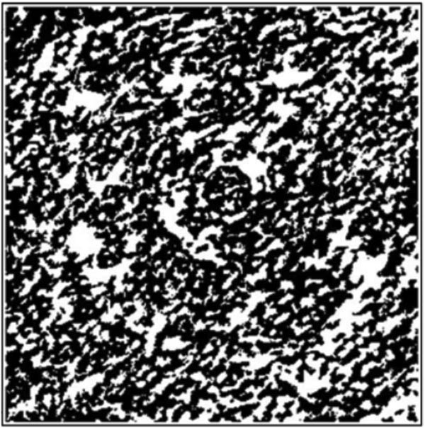
Internal structure of porous media.

3.1 Circular and square random structure

A certain number of circles with the same diameter and a number of randomly generated squares with side lengths of random numbers within a certain range are, respectively, placed in a calculation domain with a size of 200 × 200 grids to form a porous medium, and set the porosity of the two structures to be ε = 0.6. Figure 6 shows the schematic diagram of the random structure of the two.

Figure 6

Schematic diagram of circular random structure (a) and square random structure (b).

Figure 7 shows the streamline diagram of the two random structures. The Reynolds number Re is 0.6. It can be found that there is no eddy current in the two random structures, indicating that the flow is mainly determined by the viscous force. At the same stage, it can be found that due to the relatively uneven distribution of the solid framework of the circular random structure, which interferes with the internal fluid flow process, the flow lines inside the circular random structure are relatively winding, with the fluid flowing from the smaller pores into the larger pores. In contrast, the distribution of the solid framework of the square random structure is relatively uniform, and the pore size is relatively uniform, and the fluid basically flows along the nearest pore.

Figure 7

Streamline diagram of circular random structure (a) and square random structure (b).

Figure 8 shows the flow field contour map of two random structures. It can be found that the velocity distribution of the square random structure is relatively concentrated and very uniform, while the velocity distribution of the circular random structure is nonuniform in which there is a velocity peak at the large pores and the velocity at the small pores is almost close to zero.

Figure 8

Contour map of flow field of circular random structure (a) and square random structure (b).

Figure 9 shows the relationship between the dimensionless permeability of two random structures and the Reynolds number. It can be found that the flow inside the two structures conforms to Darcy’s law. The permeability of the circular random structure is greater than that of the square random structure. Figures 7 and 8 show that the distribution of the solid framework of the circular random structure is uneven, and larger pores will be formed to let most of the fluid flow through with relatively better permeability, while the distribution of the solid framework of the square random structure is relatively more uniform so as to make the pore size more consistent and cause greater fluid flow resistance. As a result, the permeability of square random structure is less than that of circular random structure.

Figure 9

The relationship between dimensionless permeability and Reynolds number of circular random structure and square random structure.

3.2 QSGS

3.2.1 Porous media constructed by QSGS

The growth core distribution probability cd represents the density of the growth core number, which reflects the statistical distribution characteristics of the growth phase in the system space. Assuming that there are 400 skeleton units in the calculation area and a 200 × 200 grid is used to construct the porous medium, the value of cd is 400/40,000 = 0.01, which means the probability that each structural node in the area becomes the growth nucleus of the skeleton is 0.01; and cd determines the fine structure characteristics of the porous medium. The larger the value, the smaller the average size of the fiber that produces the structure, and the distribution is more uniform. If the cd value is too small, there will be too few growth core under a certain number of grids, and a more realistic porous media structure cannot be formed. Figure 10 shows the porous media constructed according to different growth core distribution probabilities. The porosity ε of both (a) and (b) is 0.6, and the cd of (b) is smaller. It can be found that the internal framework and pore shape are more refined.

Figure 10

The structure of porous media with different growth core distribution probabilities by QSGS (ε = 0.6). (a) cd = 0.1 and (b) cd = 0.01

The directional growth probability di means the probability that adjacent nodes become the growth phase in the direction i. Choosing the same or different growth probabilities in each direction can construct an isotropic or anisotropic porous medium. For the D2Q9 model, the growth direction is consistent with the discrete velocity direction, and the horizontal growth probability is set to d13, the vertical direction is set to d24, and the two diagonal directions are set to d57 and d68, respectively. Figure 11 shows the pore structure of two-dimensional porous media generated according to different growth probabilities. The black parts in the figure are pores, and the white parts are the solid framework of the growth phase. It can be found that (a) has obvious isotropy, while (b), (c), and (d) have obvious anisotropy.

Figure 11

The structure of porous media with various growth probabilities by QSGS (cd = 0.01, ε = 0.3). (a) d13 = d24 = d57 = d68 = 0.001, (b) d13 = 0.08, d24 = d57 = d68 = 0.001, (c) d24 = 0.08, d13 = d57 = d68 = 0.001, and (d) d57 = 0.08, d13 = d24 = d68 = 0.001.

3.2.2 Flow analysis of QSGS with different directional growth probabilities

The QSGS is used to construct isotropic and anisotropic porous media, the porosity ε is 0.7, the growth core distribution probability cd = 0.01, and the directional growth probability di of isotropic porous media is: d13 = d24 = d57 = d68 = 0.001, the directional growth probability di of anisotropic porous media is: d13 = 0.08, d24 = d57 = d68 = 0.001, Reynolds number Re = 0.6, and the internal flow field is calculated. As shown in Figure 12, the white area is the solid framework and the colored area is the flow area. By comparing the isotropic structure with the anisotropic porous medium, it can be found that although the porosity of the two is the same, in the flow direction, the isotropic porous media structure has fewer effective paths, and most of the pore ends are closed dead ends. Figure 13 shows the average velocity in the y direction of the two. It can be found that the overall average velocity of the isotropic structure is less than the anisotropy. If x/H is smaller than 0.32, the isotropic velocity is greater than the anisotropy. This is because the isotropic structure generated in this article has more pores at the fluid inlet and the flow rate is larger. When the fluid reaches the back section of the structure, it cannot pass through, and its average velocity is lower than the anisotropic structure at the beginning.

Figure 12

Flow field contour map of QSGS with different growth probabilities. (a) d13 = d24 = d57 = d68 = 0.001 and (b) d13 = 0.08, d24 = d57 = d68 = 0.001.

Figure 13

Average velocity in y direction of flow field in porous media with isotropic and anisotropic structure.

Figure 14 shows the pressure distribution contour map of the isotropic structure. Since there are many pores at the left flow inlet, most of the fluid can flow forward, so the pressure gradient of the entire calculation area is small. At the fluid inlet, the pressure in the blue area is lower. If you zoom in on the streamline diagram here, you can find that the fluid cannot continue to flow after entering the pores here, then generate vortices and flow out of the pores. The pressure is lower compared to other areas. The pressure in the red area is significantly higher than other areas. By zooming in on the streamline diagram here, it can be found that after the fluid enters the pores here, there is a sudden narrow “throat” where the flow velocity suddenly increases. According to Darcy’s law, the pressure in the seepage area is linearly correlated with the flow velocity, so the pressure in this area becomes larger.

Figure 14

Pressure distribution contour map of isotropic porous media.

4 Three-dimensional single channel heat transfer analysis

4.1 Three-dimensional channel flow model

Due to the similarity of the internal channels of the particulate filter, a single channel is selected as the calculation domain. Figure 15 shows a schematic diagram of the established three-dimensional and two-dimensional physical model of a single channel of the particulate filter. The main geometric features used in the simulation are shown in Table 1. In order to ensure the stability of the simulation and fully develop the intake air flow, the inlet has increased the calculation area by 0.1 times the length of the channel. The channel is provided with an external flow field as the air outlet, the plug part is set as an adiabatic wall, and the surrounding walls adopt the rebound boundary format. The fluid inlet adopts velocity boundary conditions.

Figure 15

(a) Three-dimensional and (b) two-dimensional schematic diagram of single channel of particulate filter.

Table 1

Geometric characteristics and working conditions of single channel of particulate filter

Geometry model features of the channel	Unit		Working conditions
Length	mm		20
Width	mm		2
Thickness	mm		0.5
Plug thickness	mm		0.6
Wall permeability	m²	1 × 10⁻¹⁴	1 × 10⁻¹³	5 × 10⁻¹³
Initial pressure	Pa		0
Intake air temperature	K		600
Temperature outside the channel	K		400
Intake speed	m/s	1	5	20

4.2 Analysis of flow characteristics in the three-dimensional channel

Figure 16 shows the relationship between the wall seepage velocity and the pressure gradient inside and outside the wall when the inlet flow velocity is 1 m/s and the wall permeability is 1 × 10⁻¹⁴ m². It can be seen from the figure that the seepage velocity of the wall has a linear relationship with the pressure gradient. As the flow velocity increases, the pressure gradient increases, and passing through the origin indicates that the seepage flow through the wall conforms to Darcy’s law.

Figure 16

Relationship between seepage velocity of the wall and pressure gradient inside and outside the wall.

Figure 17 shows the velocity distribution in the x direction at different axial positions when the inlet air velocity is 1 m/s and the wall permeability is 1 × 10⁻¹⁴ m². It can be found that the air velocity distribution inside the channel is similar to Poiseuille flow. The distribution is parabolic; the farther away from the entrance of the channel, the lower the speed, the lowest air velocity near the wall of the channel, the highest air velocity at the center line, and the minimum seepage velocity in the porous media wall.

Figure 17

Velocity distribution in x direction at different axial positions.

Figure 18 shows the seepage velocity distribution in the porous media wall at different axial positions when the inlet air velocity is 1 m/s and the wall permeability is 1 × 10⁻¹⁴ m². It can be seen from the figure that the wall seepage at different axial positions the overall velocity is not much different, especially the seepage velocity on the side far from the flow field inside the channel is very close, the seepage velocity in the side wall close to the flow field gradually increases, and the seepage velocity near the channel entrance is relatively large.

Figure 18

Wall seepage velocity distribution at different axial positions.

4.3 Effect of intake speed on flow

Figure 19 shows a three-dimensional streamline diagram at different intake speeds. It can be seen from the figure that when the intake air velocity is low, the streamline passes through the wall and continues to flow in the original velocity direction, while the streamline with higher intake velocity still flows to the rear end of the channel after passing through the wall; when the intake air velocity is low, the streamlines are relatively regular throughout the channel, while the streamlines at high velocities become very complicated, especially at 20 m/s, a large number of vortices appear at the ends of the channel.

Figure 19

Three-dimensional streamline diagram at different intake speeds. (a) u = 1 m/s, (b) u = 5 m/s, and (c) u = 20 m/s.

Figure 20 shows the velocity contour map at different intake air flow rates. It can be found that because the frictional force of the airflow near the wall and the viscous force inside the fluid are greater than the inertial force of the airflow, the uniform flow at the entrance of the channel gradually changes into an uneven flow along the axial direction, and because of the plug at the end of the channel, the airflow cannot directly flow out of the channel, so the flow rate gradually decreases. For the inlet velocity of 1 m/s, the uniformity of the velocity field is significantly lower than that of 5 and 20 m/s, and the velocity near the end of the channel is close to zero, while for the inlet velocity of 5 and 20 m/s cases, the end of the channel has an outward velocity field. Because of its high flow rate, the airflow still has a relatively high velocity near the plug. The fluid is forced to flow through the porous media wall near the plug to the outside of the channel.

Figure 20

Velocity contour map at different intake speeds. (a) u = 1 m/s, (b) u = 5 m/s, and (c) u = 20 m/s.

Figure 21 shows the change curve of the channel centerline velocity under different intake speeds in the steady state. From the figure, it can be found that the centerline velocity distribution of the channel with the intake flow velocity of 5 and 20 m/s has similar characteristics. The mainstream velocity does not change much, but the velocity in the area near the plug quickly decreases to zero.

Figure 21

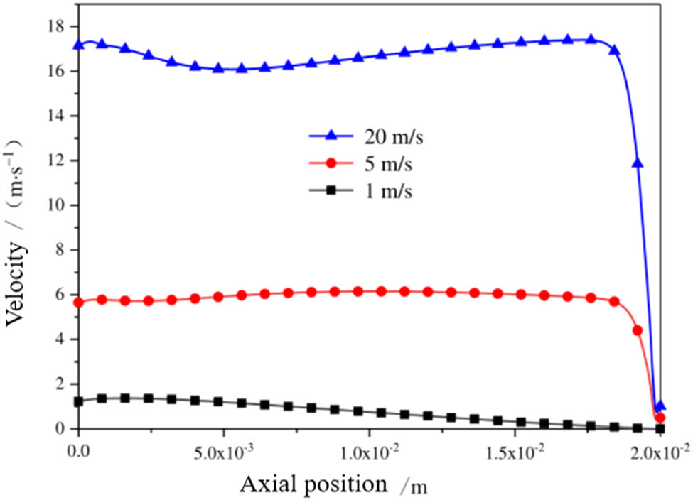
Variation curve of center line velocity of channel under different intake speeds in the steady state.

Figure 22 shows the axial change curve of the wall seepage velocity of the inlet air velocity 1 and 5 m/s, the wall permeability is 1 × 10⁻¹⁴ m², and the wall thickness is 0.45 mm.

Figure 22

Change curve of wall seepage velocity along the axial direction under different inlet velocities.

It can be seen from Figure 22 that when the intake velocity is 1 m/s, the wall seepage velocity gradually decreases along the axis, and when the intake velocity increases to 5 m/s, it can be found that the wall seepage velocity gradually increases along the axis. It means that more air flows through the wall at the rear end of the channel, which is consistent with the velocity contour maps. When the air inlet velocity is small, the pressure at the end of the channel is also small. The main driving force for the flow from the inside of the channel to the outside, the static pressure of the channel gradually increases along the axial direction, and the seepage velocity increases accordingly. The gas seepage velocity is proportional to the flow rate. The particulates will be filtered out as the gas flows through the wall of the porous medium. When the flow rate is large, it means that the number of particulates passing through the wall is also great, and the more particulates are trapped, so the value of seepage velocity can be used to measure the amount of particulates trapped. It can be inferred that the particulates deposited on the wall at the end of the channel at a higher inlet flow rate are more.

Figure 23 shows the pressure contour map inside the channel at different intake speeds. It can be found that the overall change of static pressure in the channel is small. This is because the resistance in the channel has a small influence on the pressure drop, so the static pressure inside the channel does not change much along the axial direction; as the flow rate increases, the pressure of the channel increases, especially when the air inlet speed is 5 and 20 m/s, the pressure at the end of the channel is significantly higher than the other parts of the channel.

Figure 23

Pressure contour map at different intake speeds. (a) u = 1 m/s, (b) u = 5 m/s, and (c) u = 20 m/s.

Figure 24 shows the temperature contour map inside the channel under different air inlet speeds. It can be found that the temperature field in the channel becomes more uniform as the flow rate increases. The temperature distribution of the porous media wall also appears at higher flow rates. When the flow velocity is 5 and 20 m/s, an outward temperature field appears at the end of the channel, indicating that in the heat transfer process of the channel, part of the heat is transferred to the wall of the porous medium by heat conduction and convection, and the other part flows out of the channel by mass transport. At the same time, it also shows that a larger part of the airflow chooses to pass through the wall of the porous medium at the end of the channel. It can be found that when the air intake velocity is 20 m/s, there is also a temperature distribution outside the inlet and outlet of the channel. This is because the intake air flow is large and contains more heat, so heat accumulation is formed at the inlet.

Figure 24

Temperature contour map at different intake speeds. (a) u = 1 m/s, (b) u = 5 m/s, and (c) u = 20 m/s.

4.4 Effect of wall permeability on heat transfer

Figure 25 shows the change curve of the channel center line velocity under different wall permeabilities when the inlet air flow rate is 5 m/s. It can be found from the figure that when the wall permeability is small, the channel center velocity changes approximately linearly. For larger wall permeability, the channel center velocity shows a nonlinear change. This is because when the wall permeability is low, the flow resistance of the wall is greater, and less air flow from the wall of the channel, and the air flow in the channel is more similar to the pure pipe flow, so the speed change is approximately linear. When the permeability is larger, the wall flow resistance is relatively small, and the airflow flows along the channel while flowing out of the channel through the wall seepage. There are many factors influencing the flow and the flow mechanism is more complicated, so the velocity distribution presents a nonlinear law.

Figure 25

Variation curve of center line velocity of channel under different wall permeabilities.

Figure 26 shows the change curve of the static pressure of the channel centerline under different wall permeabilities at an inlet flow rate of 5 m/s. It can be seen from the figure that as the wall permeability decreases, the static pressure in the channel increases greatly, and when the wall permeability is small, the static pressure change of the channel center is approximately linear. When the wall permeability is large, the static pressure change along the channel is small, and the pressure increases sharply only at the end of the channel.

Figure 26

Variation curve of static pressure at the center line of the channel under different wall permeabilities.

Figure 27 shows the change curve of the temperature of the channel center under different wall permeabilities when the air inlet flow rate is 5 m/s. From the figure, it can be found that the temperature of different wall permeabilities is not much different. This is because the fluid conducts little heat through the wall seepage. And most of the gas flows out of the channel on the wall near the plug. Wall permeability has little effect on the heat transfer of the channel. The heat transfer inside the channel is affected by conduction and convection. Therefore, the temperature curve in the channel is nonlinear changes. The temperature curve near the plug fluctuates. This is due to the accumulation of air flow at the plug, and more gas percolates out of the channel through the wall. The flow situation is more complicated, and the heat transfer mechanism here is also relatively complicated. Therefore, there is a certain fluctuation in temperature at the end of the channel.

Figure 27

Variation curve of center temperature of channel under different wall permeabilities.

5 Conclusions

The internal seepage laws of both the circular random structure and the square random structure constructed in this article conform to Darcy’s law. The flow characteristics of the round and square random structures are affected by the distribution of pores. The solid framework of the round random structure is unevenly distributed and form larger pores, so the permeability is relatively good. The solid framework of the square random structure is uniformly distributed and the pore size is relatively uniform, so the resistance when the fluid flows is relatively large.
The four parameters in the QSGS are the probability of growth core and the probabilities of directional growth in three directions, respectively. The greater the probability of growth core, the finer the structure of the porous media skeleton and pore shape, and the denser the skeleton. Anisotropic and isotropic porous media structure can be realized by changing different directional growth probabilities. The flow capacity of the isotropic QSGS is better than that of the anisotropic one since the flow direction is horizontal in this case.
Based on the REV scale and the flow inside a single channel of the engine particulate filter, it is found that the internal seepage flow in the channel wall conforms to Darcy’s law, and the flow inside the channel is similar to Poiseuille flow when the inlet air velocity is low. Different inlet flow rates have a significant effect on the flow and heat transfer of the channel. That is, the pressure and heat transfer intensity of the channel increase as flow rate goes up. Different wall permeability has a certain influence on the flow in the channel. That is, the smaller the wall permeability, the closer the flow is to pure pipe flow, and the less the influence of wall permeability on the heat transfer inside the channel.

tel: +86-02-26-034-5279, tel: +86-02-26-043-5784

Acknowledgments

This work was supported by the National Natural Science Foundation of China (52005149), Natural Science Foundation of Hebei Province (E2018202064), National Engineering Laboratory for Mobile Source Emission Control Technology (NELMS2017B06), and State Key Laboratory of Engines, Tianjin University (K2020-15).

References

[1] Peters A, von Klot S, Heier M, Trentinaglia I, Hormann A, Wichmann HE, et al. Exposure to traffic and the onset of myocardial infarction. J N Engl J Med. 2004;351(17):1721–30. 10.1056/NEJMoa040203.Search in Google Scholar PubMed

[2] Bernstein JA, Alexis N, Barnes C, Bernstein IL, Williams PB. Health effects of air pollution. J Allergy Clin Immunol. 2004;114(5):1116–23. 10.1016/j.jaci.2004.08.030 Search in Google Scholar PubMed

[3] Franck U, Odeh S, Wiedensohler A, Wehner B, Herbarth O. The effect of particle size on cardiovascular disorders – The smaller the worse. J Sci Total Environ. 2011;409(20):4217–21. 10.1016/j.scitotenv.2011.05.049.Search in Google Scholar PubMed

[4] Han Y, Zhu T, Guan T, Zhu Y, Liu J, Ji Y, et al. Association between size-segregated particles in ambient air and acute respiratory inflammation. J Sci Total Environ. 2016;565:412–9. 10.1016/j.scitotenv.2016.04.196.Search in Google Scholar PubMed

[5] Wang S, Yan Q, Zhang R, Jiang N, Yin S, Ye H, et al. Size-fractionated particulate elements in an inland city of China: Deposition flux in human respiratory, health risks, source apportionment, and dry deposition. J Environ Pollut. 2019;247:515–23. 10.1016/j.envpol.2019.01.051.Search in Google Scholar PubMed

[6] Guan B, Zhan R, Lin H, Huang Z. Review of the state-of-the-art of exhaust particulate filter technology in internal combustion engines. J Environ Manag. 2015;154:225–58. 10.1016/j.jenvman.2015.02.027.Search in Google Scholar PubMed

[7] Eakle S, Avery S, Weber P, Henry C. Comparison of accelerated ash loading methods for gasoline particulate filters. C SAE Technical Paper Series. 2018;2018-01-1703. 10.4271/2018-01-1703.Search in Google Scholar

[8] Yu M, Luss D, Balakotaiah V. Analysis of ignition in a diesel particulate filter. J Catal Today. 2013;216(2013):158–68. 10.1016/j.cattod.2013.05.003.Search in Google Scholar

[9] Wu G, Kuznetsov AV, Jasper WJ. Distribution characteristics of exhaust gases and soot particles in a wall-flow ceramics filter. J Aerosol Sci. 2011;42(7):447–61. 10.1016/j.jaerosci.2011.04.003.Search in Google Scholar

[10] Mizutani T, Kaneda A, Ichikawa S, Miyairi Y, Ohara E, Takahashi A. Filtration behavior of diesel particulate filters (2). C SAE Technical Paper Series. 2007;2007-01-0921. 10.4271/2007-01-0923.Search in Google Scholar

[11] Konstandopoulos AG, Kostoglou M, Housiada P, Vlachos N, Zarvalis D. Simulation of triangular-cell-shaped, fibrous wall-flow filters. C SAE Technical Paper Series. 2003;2003-01-0839. 10.4271/2003-01-0839.Search in Google Scholar

[12] Konstandopoulos AG, Kostoglou M, Vlachos N. The multiscale nature of diesel particulate filter simulation. J Int J Veh Des. 2006;41(1–4):256–84. 10.1504/ijvd.2006.009676.Search in Google Scholar

[13] Fino D, Bensaid S, Piumetti M, Russo N. A review on the catalytic combustion of soot in diesel particulate filters for automotive applications: From powder catalysts to structured reactors. J Appl Catal A: Gen. 2016;509:75–96. 10.1016/j.apcata.2015.10.016.Search in Google Scholar

[14] Zheng D, Wang J, Chen Z, Baleta J, Sundén B. Performance analysis of a plate heat exchanger using various nanofluids. J Int J Heat Mass Transf. 2020;158:119993. 10.1016/j.ijheatmasstransfer.2020.119993.Search in Google Scholar

[15] Chen Z, Zheng D, Wang J, Chen L, Sundén B. Experimental investigation on heat transfer characteristics of various nanofluids in an indoor electric heater. J Renew Energy. 2019;147(1):1011–18. 10.1016/j.renene.2019.09.036.Search in Google Scholar

[16] Kong X, Li Z, Shen B, Wu Y, Zhang Y, Cai D. Simulation of flow and soot particle distribution in wall-flow DPF based on lattice Boltzmann method. J Chem Eng Sci. 2019;202:169–85. 10.1016/j.ces.2019.03.039.Search in Google Scholar

[17] Yamamoto K, Takada N, Misawa M. Combustion simulation with lattice Boltzmann method in a three-dimensional porous structure. J Proc Combust Inst. 2005;30(1):1509–15. 10.1016/j.proci.2004.08.030.Search in Google Scholar

[18] Yamamoto K, Satake S, Yamashita H, Takada N, Misawa M. Lattice Boltzmann simulation on porous structure and soot accumulation. J Math Comp Simul. 2006;72(2–6):257–63. 10.1016/j.matcom.2006.05.021.Search in Google Scholar

[19] Yamamoto K, Takada N. LB simulation on soot combustion in porous media. J Phys A: Stat Mech Its Appl. 2006;362(1):111–7. 10.1016/j.physa.2005.09.033.Search in Google Scholar

[20] Yamamoto K, Satake S, Yamashita H. Microstructure and particle-laden flow in diesel particulate filter. J Int J Therm Sci. 2009;48(2):303–7. 10.1016/j.ijthermalsci.2008.08.009.Search in Google Scholar

[21] Lee DY, Lee GW, Yoon K, Chun B, Jung HW. Lattice Boltzmann simulations for wall-flow dynamics in porous ceramic diesel particulate filters. J Appl Surf Sci. 2018;429:72–80. 10.1016/j.apsusc.2017.08.074.Search in Google Scholar

[22] Wolf-Gladrow DA. Lattice Gas cellular automata and lattice Boltzmann models. New York: Springer; 2000. 10.1007/b72010.Search in Google Scholar

[23] Qian YH, Orszag SA, Lattice BGK. Models for the Navier–Stokes equation: Nonlinear deviation in compressible regimes. Europhys Lett. 1993;21(3):255–9. 10.1209/0295-5075/21/3/001.Search in Google Scholar

[24] Peng Y, Shu C, Chew YT. Simplified thermal lattice Boltzmann model for incompressible thermal flows. J Phys Rev E. 2003;68(2);026701-1–026701-8. 10.1103/physreve.68.026701.Search in Google Scholar PubMed

[25] Shan X. Simulation of Rayleigh–Bénard convection using a lattice Boltzmann method. J Phys Rev. 1997;55:2780–8. 10.1103/physreve.55.2780.Search in Google Scholar

[26] He X, Chen S, Doolen GD, Novel A. Thermal model for the lattice Boltzmann method in incompressible limit. J Comput Phys. 1998;146:282–300. 10.1006/jcph.1998.6057.Search in Google Scholar

[27] Mei R, Shyy W, Yu D, Luo LS. Lattice Boltzmann method for 3-D flows with curved boundary. J Computat Phys. 2000;161(2):680–99. 10.1006/jcph.2000.6522.Search in Google Scholar

[28] He X, Luo LS. Theory of the lattice Boltzmann method: From the Boltzmann equation to the lattice Boltzmann equation. J Phys Rev E. 1997;56(6):6811–7. 10.1103/physreve.56.6811.Search in Google Scholar

[29] Bear J. Dynamics of fluids in porous media. M Soil Sci. 1975;120(2):162–3. 10.1097/00010694-197508000-00022.Search in Google Scholar

[30] Ritzi RW, Bobeck P. Comprehensive principles of quantitative hydrogeology established by Darcy (1856) and Dupuit (1857). J Water Resour Res. 2008;44(10):12–25. 10.1029/2008wr007002.Search in Google Scholar

[31] Zhang M, Ye G, Breugel Kvan. Microstructure-based modeling of permeability of cementitious materials using multiple-relaxation-time lattice Boltzmann method. J Computat Mater Sci. 2013;68:142–51. 10.1016/j.commatsci.2012.09.033.Search in Google Scholar

[32] Wang J, Tian K, Zhu H, Zeng M, Sundén B. Numerical investigation of particle deposition in film-cooled blade leading edge. J Numer Heat Transfer, Part A: Appl. 2020;77(20):579–98. 10.1080/10407782.2020.1713692.Search in Google Scholar

[33] Kong X, Li Z, Cai D, Shen B, Zhang Y. Numerical simulation of the particle filtration process inside porous walls using lattice Boltzmann Method. J Chem Eng Sci. 2019;202:282–99. 10.1016/j.ces.2019.03.040.Search in Google Scholar

[34] Wang M, Wang J, Pan N, Chen S. Mesoscopic predictions of the effective thermal conductivity for microscale random porous media. J Phys Rev E. 2007;75(3):036702. 10.1103/physreve.75.036702.Search in Google Scholar

[35] Wang M, Pan N, Wang J, Chen S. Mesoscopic simulations of phase distribution effects on the effective thermal conductivity of microgranular porous media. J Colloid Interface Sci. 2007;311(2):562–70. 10.1016/j.jcis.2007.03.038.Search in Google Scholar PubMed

[36] Wang M, Pan N. Numerical analyses of effective dielectric constant of multiphase microporous media. J Appl Phys. 2007;101(11):114102. 10.1063/1.274373.Search in Google Scholar

Received: 2020-09-15

Revised: 2020-11-03

Accepted: 2020-11-04

Published Online: 2020-12-05

This work is licensed under the Creative Commons Attribution 4.0 International License.

Articles in the same Issue

https://doi.org/10.1515/phys-2020-0208

Keywords for this article

particulate filters; porous media; lattice Boltzmann method; single channel; multi-scale

Creative Commons

BY 4.0