
Introduction to disoriented knot theory
-
İsmet Altıntaş


Abstract
This paper is an introduction to disoriented knot theory, which is a generalization of the oriented knot and link diagrams and an exposition of new ideas and constructions, including the basic definitions and concepts such as disoriented knot, disoriented crossing and Reidemesiter moves for disoriented diagrams, numerical invariants such as the linking number and the complete writhe, the polynomial invariants such as the bracket polynomial, the Jones polynomial for the disoriented knots and links.
1 Introduction
This paper gives an introduction to the subject of disoriented knot theory. We introduce the notion of a disoriented crossing and explain how to adapt the fundamental concepts and invariants of the knot theory to a setting in which we have disoriented crossing.
The disoriented knot and link diagrams arise when calculating the Jones [1, 2], HOMFLY [3] polynomials etc., using the oriented diagram structure of the state summation for the oriented knot and link diagrams. When we split a crossing of an oriented knot diagram using Kauffman’s bracket model [4, 5], one of the occurring diagram is a disoriented diagram. Since the disoriented diagrams acquire orientations outside the category of knot and link diagrams, only unoriented and oriented knot and link diagrams have previously been considered in the literature for the development of knot theory.
In this paper, we put disoriented knot and link diagrams on the same footing as oriented knot and link diagrams. We define the concepts of a disoriented diagram and a disoriented crossing and give the Reidemeister moves for disoriented diagrams. We see that most classic basic concepts of knot theory are not invariant for the disoriented diagrams of a knot or link. Here, we redefine the linking number for the disoriented link diagrams and prove that the linking number is a link invariant of the link. We define a new concept called complete writhe instead of the classic writhe that is not a regular isotopy invariant for disoriented link diagrams. Thus, the normalized bracket polynomial (the Jones polynomial) by the complete writhe for disoriented link diagrams will be an invariant of the link.
The paper is organized as follows. Section 2 gives the definitions of the disoriented knot and link diagrams and disoriented crossing. In this section, we also give the brief description about of disoriented diagrams and the Reidemeister moves on the disoriented diagrams.
Sections 3 and 4 contain some numerical invariants. In Section 3, we define the linking number for the disoriented link diagrams, prove that the linking number is a link invariant and give two examples. In Section 4, we adapt the writhe for the disoriented knot and link diagrams. We define a new concept called complete writhe for the disoriented knot and link diagrams and prove that the complete writhe is invariant under the Reidemeister moves RII and RIII for the disoriented diagrams.
Section 5 presents a review of the bracket polynomial [4, 5, 6] and the Jones polynomial for the disoriented knot and link diagrams. We expand the bracket polynomial for disoriented diagrams of a knot (or link). So, the normalized bracket polynomial can also be extended for the disoriented knot and link diagrams. Since the normalized bracket polynomial (the Jones polynomial) is invariant under the first Reidemeister move for oriented knot diagrams, it is a stronger invariant than regular isotopy invariant for the disoriented diagrams. However, the Jones polynomial is not invariant under all the moves on disoriented diagrams. Therefore, it is not an invariant for the disoriented knot and link diagrams. In this section, we redefine the Jones polynomial for the disoriented knot and link diagrams by using complete writhe. This polynomial called the complete Jones polynomial is invariant under all the moves on disoriented diagrams. Thus it is a knot and link invariant. Moreover, the complete Jones polynomial of each disoriented diagram of a knot is equal to the original Jones polynomial of the knot. The last part of this section contains a few examples.
2 Defining disoriented knots and links
A knot is an embedding of a circle in three dimensional space ℝ3 (or S3). An oriented knot is a knot diagram which has been given an orientation. Taking into account the facts about the embedding, we can also define an oriented knot as an embedding of an oriented circle in three dimensional space. In a similar way, we define a disoriented knot.
Definition 2.1
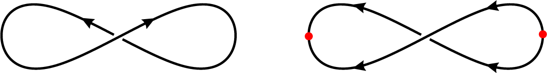
A disoriented circle is a circle upon which we have chosen two points, and have chosen an orientation of both of the arcs between those two points. We allow that the orientation of one of the arcs is the reverse of the orientation of the other.
A few simple disoriented diagrams, a disoriented circle and their replacements have been illustrated in Fig. 1. The basic reduction move in Fig. 1 corresponds to elimination of two consecutive cusps on a simple loop. Note that it is allowed to the cancelation of consecutive cusps along a loop where the cusps both points to the same local region of the two local regions delineated by the loop but not allowed to the cancelation of a “zig-zag” where two consecutive cusps point to opposite local sides of the loop. A zig-zag is represented an oriented or disoriented virtual crossing of the oriented or disoriented diagram of a knot and link. Since we work on the classical knot and link diagrams in this paper, we do not encounter a zig-zag. Thus, for we can easily draw a disoriented knot or link diagram, we use the local disoriented curve of the form  instead of the cusp with two points of the form
  . Due to our present disclosure, a disoriented curve can be replaced with an oriented curve. Likewise, a disoriented circle can be replaced with an oriented circle. For detailed information about disoriented configurations, replacements and disoriented relations can be seen in [7, 8, 9, 10, 11].
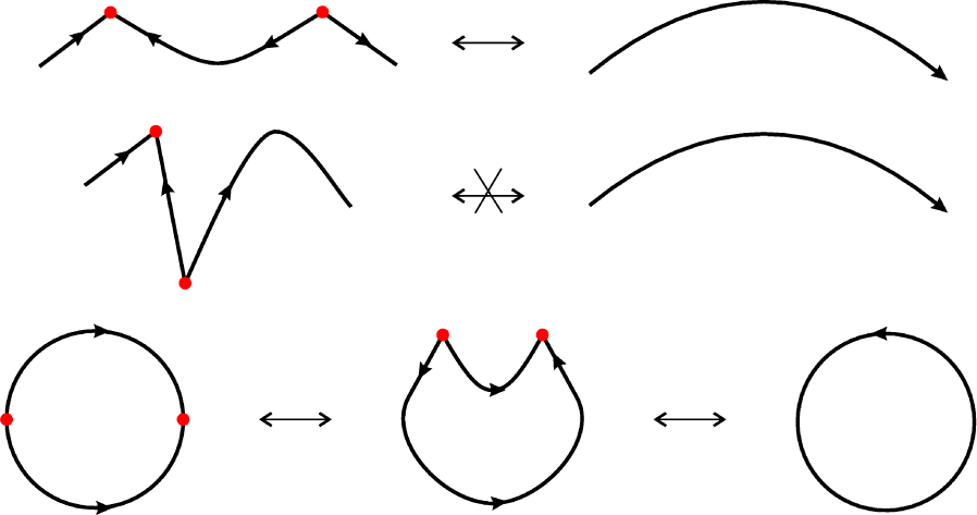
Simple Disoriented Diagrams and Replacements.
Definition 2.2
A disoriented knot is an embedding of a disoriented circle in three dimensional space ℝ3(or S3). A disoriented link of k-components is an embedding of a disjoint union of k circles in ℝ3, where at least one of circles is disoriented. Two disoriented knots equivalent if there is a continuous deformation of ℝ3taking one to the other.
If K a disoriented knot (or link) in ℝ3, its projection is π(K) ⊂ ℝ2, where π is the projection along the z-axis onto the xy-plane. The projection is said to be regular projection if the preimage of a point of π(K) consists of either one or two points of K. If K has a regular projection, then we can define the corresponding disoriented diagram D by redrawing it with an arc near crossing (the place with two preimages in K) to incorporate the overpass/underpass information.
Definition 2.3
A crossing of a disoriented knot K is disoriented if the overpass and underpass arcs of the crossing have opposite orientations. In other words, if A1and A2are the arcs of the disoriented circle of which K is an embedding, then one of the underpass and overpass arcs is A1, and the other is A2. If a crossing of a disoriented knot K is not disoriented, we say that it is oriented. An oriented knot is a disoriented knot with zero disoriented crossing. For example, see Fig. 3.
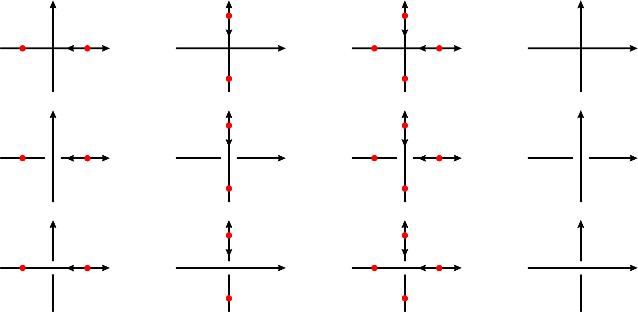
Disoriented and Oriented Crossings.
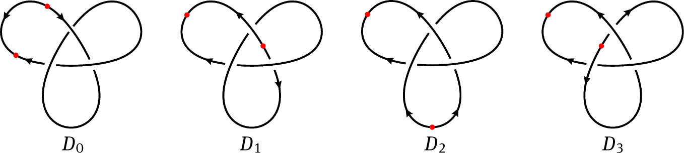
Disoriented Diagrams of the right-hand trefoil.
Definition 2.4
Let L be a link with exactly two components, K1and K2. Choose a disorientation of both K1and K2. Denote the two arcs of K1by
One of the underpass and overpass arcs of the crossings is
One of the underpass and overpass arcs of the crossings is
Otherwise, we say that the crossing is oriented.
Remark 2.5
Similar considerations apply to disoriented links with more than two components. We have not discussed here to avoid going beyond the purpose of the paper.
Although the underpass and overpass of an oriented crossing are the same with the underpass and overpass of a disoriented crossing, the sings of these crossings are not the same. Then, a disoriented crossing can not be replaced with an oriented crossing. We illustrate oriented and disoriented crossings in Fig. 2.
The Reidemeister moves on disoriented diagrams generalize the Reidemeister moves for the oriented knot and link diagrams. We illustrate the Reidemeister moves on disoriented diagrams in Fig. 4, 5 and 6. The Reidemeister moves of types II and III for oriented diagrams are expanded on disoriented diagrams. A new disoriented curled move is added to Reidemeister move of type I for disoriented diagrams. Disoriented knot and link diagrams that can be connected by a finite sequence of these moves and their inverse moves are said to be equivalent. We list the equivalence of these Reidemesiter moves illustrated in Fig. 4, 5 and 6 as below:
Planar and First Reidemeister Moves for Disoriented Diagrams.
Second Reidemeister Moves for Disoriented Diagrams.
Third Reidemeister Moves for Disoriented Diagrams.
Remark 2.6
Note that there are many other possible choices of the orientation of the arcs in Fig. 6.
We call regular isotopy to the equivalence relation generated by the moves RII and RIII (and the planar moves), ambient isotopy to the equivalence relation generated by the moves RI, RII and RIII, and complete ambient isotopy to the equivalence relation on disoriented diagrams that is generated by all the moves in Fig. 4, 5 and 6. Since there is no disoriented crossing of an oriented diagram, the complete ambient isotopy is equivalent to the ambient isotopy on the oriented diagrams. But, the complete ambient isotopy is more powerful than the ambient isotopy for the disoriented knot and link diagrams.
3 Linking number
In this section, we define the linking number for disoriented links and prove that the linking number of a disoriented link is its invariant.
Definition 3.1
Let L be a disoriented link with two components K1and K2. The linking number lk(L) is defined by formula
where K1 ⊓ K2denotes the set of crossings of K1with K2(no self-crossings), where the first sum runs over the oriented crossings of K1 ⊓ K2, the second sum runs over the disoriented crossings of K1 ⊓ K2, and ε(o) and ε(d) denote the sign of an oriented crossing and the sign of a disoriented crossing of belonging to K1 ⊓ K2, respectively.
The following theorem gives that the linking numbers of all the disoriented diagrams of a link are equal.
Theorem 3.2
The linking number lk(L) is an invariant of the link L.
Proof
Let D be a disoriented regular diagram of the link L with two components. We suppose that D′ is another regular diagram of L. From our discussions so far, we know that we may obtain D′ by performing, if necessary several times, the Reidemeister moves in Fig. 4, 5 and 6. Therefore, in order to prove the theorem, it is sufficient to show that the value of the linking number remains unchanged after each of the Reidemeister moves is performed on D.
The move RI: At the crossings of D at which we intend to apply the move RI, every section (edge) of such a crossing belongs to the same component. Therefore, applying the move RI does not affect the calculation of the linking number. In the same way, the move RI′ does also not affect the calculation of the linking number.
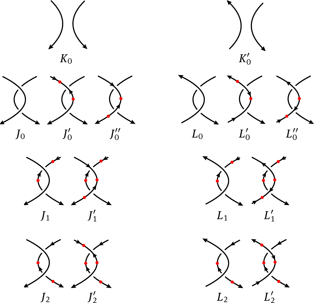
The moves RII: We shall only examine the effects of the cases
Some Second Reidemeister Moves.
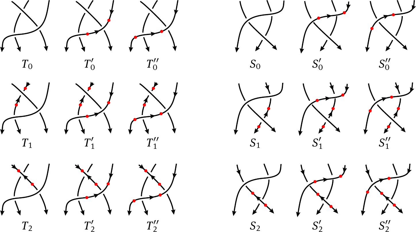
The moves RIII: Finally, let us consider the effect of the moves RIII on D. We only consider the effect of the cases T0 and S0,
Some Disoriented Third Reidemeister Moves.
To be identical the effects of the cases Ti and Si, the following equations should always be hold:
If all crossings are oriented or disoriented,
If one of the crossings c2 and
or
If one of the crossings c2 and
If A, B and C belong to the same component for the only case in Fig. 8, then the linking number is unaffected. So we suppose that A belong to a different component than B and C. Then the parts that have an effect on linking number is the sum of the signs of the crossings c1, c2 and
by Definition 3.1. Since the crossing
Since the crossing
Since the crossing c1 and
Thus, none of the sums does cause any change to the linking number. The other cases, (i.e. the various possibilities for the components that A, B and C belong to) can be treated in a similar manner. The remaining cases of the moves RIII can be examined in a similar way. Hence, the linking number remains unchanged when we apply the moves RIII. □
We suppose now that L is a disoriented link with n components, K1, K2, …, Kn With regard to two components, Ki and Kj, i < j, we may define as an extension of the linking number lk(L) = lk(Ki, Kj), 1 ≤ i < j ≤ n This approach will give us n(n − 1)/2 linking numbers, and their sum,
is called the total linking number of K. One can show that, in fact, the total linking number of K is an invariant of K.
Remark 3.3
The disoriented linking number is always equal to the oriented linking number, regardless of the choice of disorientation. Indeed, if one can change the sign of an oriented crossing by making disoriented, then it will be changed back again in the sum defining the linking number.
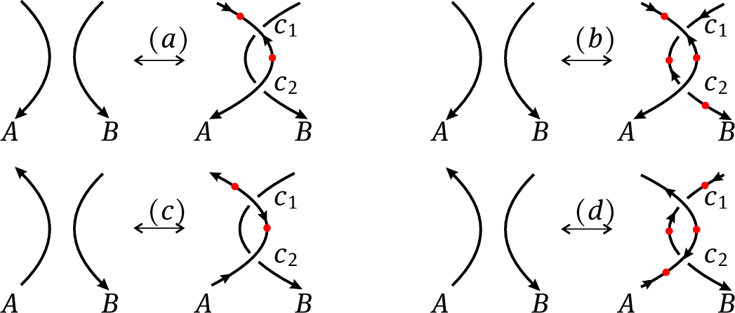
Example 3.4
Let L be any disoriented diagram of unlink in Fig. 9. In the case (a), there are two oriented crossings which have the opposite sign. So, ε(o) = 0. In the cases (b) and (c), there are a disoriented crossing and an oriented crossing which have the same sign. So, ε(o) – ε(d) = 0. In the case (d), there are two disoriented crossings which have the opposite sign. So, ε(d) = 0. Thus, in each case, we get lk(L) = 0.
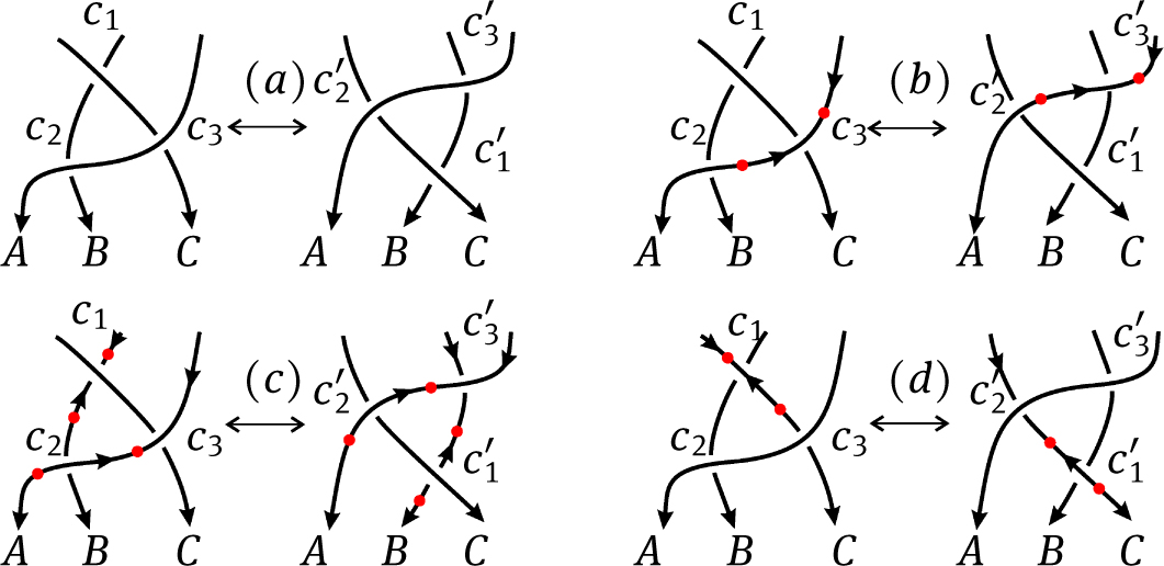
Let L be any disoriented diagram of link in Fig. 10. In the case (a), there are two oriented crossings which have the same sign. So, ε(o) = 2. In the cases (b) and (c), there are a disoriented crossing and an oriented crossing which have the opposite sign. So, |ε(o) − ε(d) | = 2. In the case (d), there are two disoriented crossings which have the negative sign. So, ε(d) = −2 and | ε(o) − ε(d) | = 2. Thus, in each case, we get lk(L) = 1.
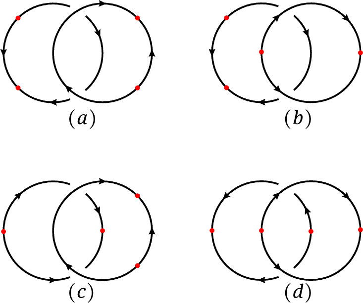
Some Disoriented Diagrams of Unlink
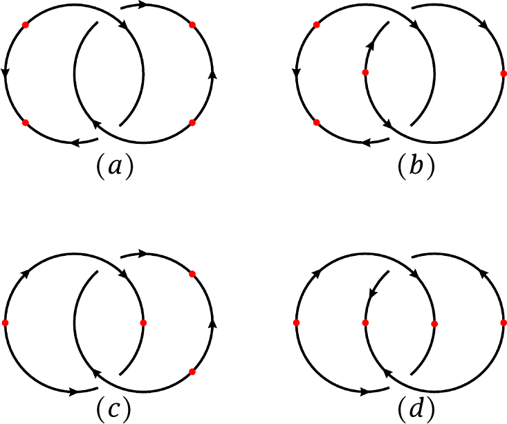
Some Disoriented Diagrams of Hopf Link
4 Writhe
Recall that the classical writhe w(D) of a regular diagram D of a knot (or a link) is the sum of the signs of all the crossings of D. This definition of the writhe can be also adapted to disoriented diagram D of a knot. The classical writhe is not a knot invariant. However, regularly isotopic oriented knot diagrams have the same writhe. It can be easily understood that the classical writhe is not invariant under the moves RII and RIII for disoriented diagrams.
Now, we define a new writhe called complete writhe for a disoriented diagram of a knot or link and prove that the complete writhes of all the disoriented diagram of a knot are equal.
Definition 4.1
Let D be a disoriented regular diagram of a knot (or link) K. The complete writhe of D, cw(D), is defined by formula
where the first sum runs over the oriented crossings of D, the second sum runs over the disoriented crossings of D and ε(o) and ε(d) denote the sign of an oriented crossing and the sign of a disoriented crossing of belonging to D, respectively.
Theorem 4.2
The complete writhe cw(D) is a regular isotopy invariant of the disoriented diagram D.
Proof
If the proof of Theorem 3.2 is adopted for all crossings of the disoriented diagram D, it is easy to see that the effects of the moves RII and RIII on the linking number are identical to those on the complete writhe cw(D). □
The complete writhe cw(D) of a disoriented diagram D is not invariant under the moves RI and RI′.
Theorem 4.3
The complete writhes of all the disoriented diagrams of a non-trivial knot (or non-trivial link) are same.
Proof
Let K be non-trivial knot (or non-trivial link) of n crossings. We denote an oriented diagram of the knot K by D0. Let cw(D0) = k, k ∈ ℤ. Let k1 be the sum of the positive signs of the crossings in the diagram D0 and k2 be the sum of the negative signs of the crossings in D0. Then, we have
Now, let D1 denotes a disoriented diagram with one disoriented crossing. If the sign of the disoriented crossing is negative, by definition of complete writhe
If the sign of the disoriented crossing is positive,
Similarly, let Dm denotes a disoriented diagram of the knot K, where the sum of the signs of disoriented crossings of Dm is m ≤ k. If m is positive,
and if m is negative,
Thus, for every disoriented diagram, D of the knot K, we have cw(D) = k, k ∈ ℤ. □
Remark 4.4
It can be understood from the proof of Theorem 4.3 that the complete writhe of any disorientation is equal to the classical writhe with respect to an orientation.
As shown in the following example, all the disoriented diagrams of a knot have the same complete writhe, although each disoriented diagram of it has a different writhe.
Example 4.5
For disoriented diagrams drawn in Fig. 3 of the right-hand trefoil, we have w(D0) = 3, w(D1) = 1, w(D2) = −1, w(D3) = −3 and cw(Di) = 3, i ∈ {0, 1, 2, 3}.
5 Polynomial invariants for disoriented knot diagrams
In this section, we give the bracket polynomial and the normalized bracket polynomial for disoriented knots and links. We show that the bracket polynomial is a regular isotopy invariant for disoriented knots and links. But, the normalized bracket polynomial is not an invariant for disoriented knots and links. For the normalized bracket polynomial to be an invariant of the disoriented knot we redefine the original normalized bracket polynomial by considering the notion of disoriented crossing that we call the complete normalized polynomial or the complete Jones polynomial. The construction of the complete normalized polynomial invariant begins with the disoriented summation of the bracket polynomial. This means that each local smoothing is either an oriented smoothing or a disoriented smoothing as illustrated in Fig. 11. The sufficient information about these smoothings can be found in Kauffman’s works [7, 9]. The bracket expansion for the crossings with both positive and negative sign in an oriented knot and link diagram can be written as an oriented bracket state model:
where K+, K−, K0 and K∞ are diagrams in Fig. 11, ◯ and D is an oriented diagram with zero-crossing of unknot and an oriented knot or link diagram, respectively and ⊔ denotes disjoint union.
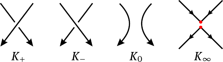
Crossings and Smoothings.
We can use this model for both oriented and disoriented crossings in a disoriented knot and link diagram. We call the extended bracket polynomial which we have obtained polynomial from the model (1) for the disoriented knot and link diagrams. As in the standard bracket polynomial, in corresponding disoriented state summation expansion of the extended bracket polynomial we have
where S runs over the oriented and the disoriented bracket states of the disoriented diagram D, 〈 D|S〉 is the usual product of vertex weights and ∣ S ∣ is the number of the circle in the state S.
Theorem 5.1
The extended bracket polynomial is a regular isotopy invariant for the disoriented knot and link diagrams.
Proof
The proof is the same as oriented ones. The proof for oriented link diagrams given in [7]. □
The extended bracket polynomial is not an invariant of the moves RI and RI′ for the disoriented knot and link diagrams. Its behavior under these moves is examined in the following lemma.
Lemma 5.2
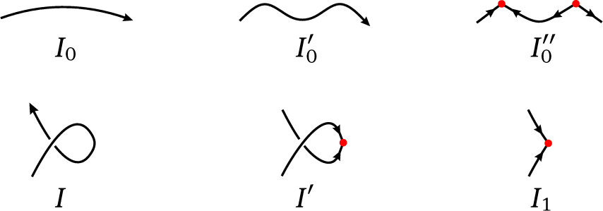
〈 I 〉 = (−A3)〈 I0〉 and 〈 I′〉 = (−A3)〈 I1〉, where I, I0, I′ and I1are local diagrams given Fig. 4.
Proof
From Fig. 12, we obtain easily 〈 I 〉 = (Aδ+A−1)〈 I0 〉 = (−A3)〈 I0〉 and 〈 I′〉 = (A−1+Aδ)〈 I1〉 = (−A3)〈 I1〉. Note that I and I′ have the opposite signs. □
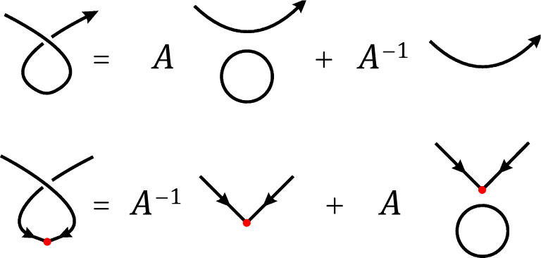
Oriented and Disoriented First Reidemeister Move.
The extended bracket polynomial is normalized to an invariant fD(A) of all oriented and disoriented moves except the RI′ move by the formula
where w(D) is the writhe of the disoriented diagram D. The polynomial fD(A) is the extension of the normalized bracket polynomial by Kauffmann [4, 5] to disoriented knot and link diagrams. The Jones polynomial, VD(t) is given in terms of this model by the formula
This definition is a direct extension to the disoriented knot and link category of the state sum model for the original Jones polynomial. It is straightforward to verify the invariances stated above, see [4, 5]. In this way, we have the Jones polynomial for the disoriented knot and link diagrams. The original Jones polynomial is not an invariant for the disoriented links. Indeed, it is not invariant under the RI′ move, see Example 5.7.
We now redefine the normalized bracket polynomial for the disoriented knot and link diagrams that we call the complete normalized polynomial and show that the complete normalized polynomial is invariant under all the moves of the disoriented knot and link diagrams.
Definition 5.3
We define a polynomial 𝓣K ∈ ℤ[A, A−1] for a disoriented diagram D of a knot (or link) K by the formula
where cw(D) is the complete writhe of disoriented diagram D. We call 𝓣Kthe complete normalized polynomial of the extended bracket polynomial by the complete writhe.
Theorem 5.4
The complete normalize polynomial is a complete ambient isotopy invariant for the disoriented knot and link diagrams.
Proof
Since cw(D) is a regular isotopy invariant, so (−A3)−cw(D), and 〈 D 〉 is also a regular isotopy invariant, it is follows that 𝓣K is a regular isotopy invariant. Thus we need check that 𝓣K is invariant under the moves RI and RI′ on disoriented diagrams. Since cw(I) = ε(o) − ε(d) = 1 − 0 = 1 and cw(I′) = 0 − (−1) = 1, and so cw(I) = 1+cw(I0) and cw(I′) = 1+cw(I1), where I, I′, I0 and I1 are diagrams given in Fig. 4, this follows at once. Indeed,
□
Finally, we have the particularly important behavior of the polynomials 〈 K 〉, fK and 𝓣K under mirror images:
Proposition 5.5
Let K*denotes the mirror image of the (disoriented) knot and link K that is obtained by switching all the crossing of K. Then 〈 K*〉(A) = 〈 K 〉(A−1), fK*(A) = fK(fA−1) and 𝓣K*(A) = 𝓣K(A−1).
Proof
Reserving all crossings exchanges the roles of A and A−1 in the definition of 〈 K 〉, fK and 𝓣K. □
Next, we show that 𝓣K is the Jones polynomial via the complete writhe. We call this polynomial as complete Jones polynomial for the disoriented knot and link diagrams and denote 𝓥K.
Theorem 5.6
The complete normalize polynomial 𝓣Kyields the complete Jones polynomial, 𝓥K(t). That is, 𝓣K(t−1/4) = 𝓥K(t).
Proof
Since the complete writhes of all the disoriented diagrams of K are equal by Theorem 4.3, we have that the complete normalized polynomial are equal for all choice of disorientation. From Remark 4.4, we obtain that the complete normalized polynomial of K is equal to the Kauffman polynomial of K. By Theorem 5.2. in [5], 𝓣K(t−1/4) = 𝓥K(t). □
Example 5.7
Let ◯1 and ◯2denotes the oriented and the disoriented diagrams of the unknot illustrated in Fig. 13, respectively. Then,
An Oriented and a Disoriented Unknot Diagram With One Crossing.
With A = t−1/4, V◯2 = t−3/2and 𝓥◯2 = 1.
Example 5.8
For the disoriented diagrams of the right hand trefoil in Fig. 3,
With A = t−1/4,
6 Discussion
In this paper, we have given an introduction to the subject of the disoriented knot theory and we have explained how to adapt the Reidemeister moves, the linking number, the writhe, the bracket polynomial and the Jones polynomial to the disoriented knot and link diagrams. We have based our work on disorientation. We have defined a new writhe called complete writhe and redefined the Jones polynomial for the disoriented knots and links diagrams. This paper lays the foundation for future works on these ideas.
Acknowledgement
The author wishes to express his gratitude to the reviewers for the many helpful and stimulating suggestions that improve the quality of this paper.
References
[1] Jones V. F. R., A new knot polynomial and von Neumann algebra, Notices Amer. Math. Soc., 1986, 33, 219–225.Search in Google Scholar
[2] Jones V. F. R., Hecke algebra representations of braid groups and link polynomials, Ann. Math., 1987, 126, 335–388.10.1142/9789812798329_0003Search in Google Scholar
[3] Freyd P., Yetter D., Hoste J., Lickoricsh W. B. R., Millett K., Ocneau A., A new polynomial invariant of knots and links, Bul. Amer. Math. Soc., 1985, 12, 239–246.10.1142/9789812798329_0002Search in Google Scholar
[4] Kauffman L. H., State models and the Jones polynomial, Topology, 1987, 26, 395–407.10.1142/9789812798329_0010Search in Google Scholar
[5] Kauffman L. H., Knot and physics, 3rd edition, Series on Knots and Everything: Volume 1, Word Scientific, Singapore, 2001.10.1142/4256Search in Google Scholar
[6] Kauffman L. H., New invariants in the theory of knots, Amer. Math. Monthly, 1988, 95, 195–242.10.1080/00029890.1988.11971990Search in Google Scholar
[7] Kauffman L. H., An extended bracket polynomial for virtual knots and links, J. Knot Theory Ramifications, 2009, 18, 1369–1422.10.1142/S0218216509007543Search in Google Scholar
[8] Kauffman L. H., Introduction to virtual knot theory, J. Knot Theory Ramifications, 2012, 21, 37 pp.10.1142/9789814313001_0019Search in Google Scholar
[9] Dye H. A., Kauffman L. H., Virtual crossing number and the arrow polynomial, J. Knot Theory Ramifications, 2009, 18, 1335–1357.10.1142/S0218216509007166Search in Google Scholar
[10] Dye H. A., Kauffman L. H., Manturov V. O., On two categorifications of the arrow polynomial for virtual knots, In: The mathematics of knots, Contrib. Math. Comput. Sci., 1, Springer, Heidelberg, 2011, 95–124.10.1007/978-3-642-15637-3_4Search in Google Scholar
[11] Clark D., Morrison S., Walker K., Fixing the functoriality of Khovanov homology, Geom. Topol., 2009, 13, 1499–1582.10.2140/gt.2009.13.1499Search in Google Scholar
[12] Murasugi K. (Translated by Bohdan Kurpita), Knot theory and its applications, Modern Birkhäuser Classics, Birkhäuser, Boston, Inc., Boston, MA, 2008.10.1007/978-0-8176-4719-3Search in Google Scholar
[13] Adams C. C., The knot book. An elementary introduction to the mathematical theory of knot, American Mathematical Society, Providence, RI, 2004.Search in Google Scholar
© 2018 Altıntaş, published by De Gruyter
This work is licensed under the Creative Commons Attribution-NonCommercial-NoDerivatives 4.0 License.
Articles in the same Issue
- Regular Articles
- Algebraic proofs for shallow water bi–Hamiltonian systems for three cocycle of the semi-direct product of Kac–Moody and Virasoro Lie algebras
- On a viscous two-fluid channel flow including evaporation
- Generation of pseudo-random numbers with the use of inverse chaotic transformation
- Singular Cauchy problem for the general Euler-Poisson-Darboux equation
- Ternary and n-ary f-distributive structures
- On the fine Simpson moduli spaces of 1-dimensional sheaves supported on plane quartics
- Evaluation of integrals with hypergeometric and logarithmic functions
- Bounded solutions of self-adjoint second order linear difference equations with periodic coeffients
- Oscillation of first order linear differential equations with several non-monotone delays
- Existence and regularity of mild solutions in some interpolation spaces for functional partial differential equations with nonlocal initial conditions
- The log-concavity of the q-derangement numbers of type B
- Generalized state maps and states on pseudo equality algebras
- Monotone subsequence via ultrapower
- Note on group irregularity strength of disconnected graphs
- On the security of the Courtois-Finiasz-Sendrier signature
- A further study on ordered regular equivalence relations in ordered semihypergroups
- On the structure vector field of a real hypersurface in complex quadric
- Rank relations between a {0, 1}-matrix and its complement
- Lie n superderivations and generalized Lie n superderivations of superalgebras
- Time parallelization scheme with an adaptive time step size for solving stiff initial value problems
- Stability problems and numerical integration on the Lie group SO(3) × R3 × R3
- On some fixed point results for (s, p, α)-contractive mappings in b-metric-like spaces and applications to integral equations
- On algebraic characterization of SSC of the Jahangir’s graph 𝓙n,m
- A greedy algorithm for interval greedoids
- On nonlinear evolution equation of second order in Banach spaces
- A primal-dual approach of weak vector equilibrium problems
- On new strong versions of Browder type theorems
- A Geršgorin-type eigenvalue localization set with n parameters for stochastic matrices
- Restriction conditions on PL(7, 2) codes (3 ≤ |𝓖i| ≤ 7)
- Singular integrals with variable kernel and fractional differentiation in homogeneous Morrey-Herz-type Hardy spaces with variable exponents
- Introduction to disoriented knot theory
- Restricted triangulation on circulant graphs
- Boundedness control sets for linear systems on Lie groups
- Chen’s inequalities for submanifolds in (κ, μ)-contact space form with a semi-symmetric metric connection
- Disjointed sum of products by a novel technique of orthogonalizing ORing
- A parametric linearizing approach for quadratically inequality constrained quadratic programs
- Generalizations of Steffensen’s inequality via the extension of Montgomery identity
- Vector fields satisfying the barycenter property
- On the freeness of hypersurface arrangements consisting of hyperplanes and spheres
- Biderivations of the higher rank Witt algebra without anti-symmetric condition
- Some remarks on spectra of nuclear operators
- Recursive interpolating sequences
- Involutory biquandles and singular knots and links
- Constacyclic codes over 𝔽pm[u1, u2,⋯,uk]/〈 ui2 = ui, uiuj = ujui〉
- Topological entropy for positively weak measure expansive shadowable maps
- Oscillation and non-oscillation of half-linear differential equations with coeffcients determined by functions having mean values
- On 𝓠-regular semigroups
- One kind power mean of the hybrid Gauss sums
- A reduced space branch and bound algorithm for a class of sum of ratios problems
- Some recurrence formulas for the Hermite polynomials and their squares
- A relaxed block splitting preconditioner for complex symmetric indefinite linear systems
- On f - prime radical in ordered semigroups
- Positive solutions of semipositone singular fractional differential systems with a parameter and integral boundary conditions
- Disjoint hypercyclicity equals disjoint supercyclicity for families of Taylor-type operators
- A stochastic differential game of low carbon technology sharing in collaborative innovation system of superior enterprises and inferior enterprises under uncertain environment
- Dynamic behavior analysis of a prey-predator model with ratio-dependent Monod-Haldane functional response
- The points and diameters of quantales
- Directed colimits of some flatness properties and purity of epimorphisms in S-posets
- Super (a, d)-H-antimagic labeling of subdivided graphs
- On the power sum problem of Lucas polynomials and its divisible property
- Existence of solutions for a shear thickening fluid-particle system with non-Newtonian potential
- On generalized P-reducible Finsler manifolds
- On Banach and Kuratowski Theorem, K-Lusin sets and strong sequences
- On the boundedness of square function generated by the Bessel differential operator in weighted Lebesque Lp,α spaces
- On the different kinds of separability of the space of Borel functions
- Curves in the Lorentz-Minkowski plane: elasticae, catenaries and grim-reapers
- Functional analysis method for the M/G/1 queueing model with single working vacation
- Existence of asymptotically periodic solutions for semilinear evolution equations with nonlocal initial conditions
- The existence of solutions to certain type of nonlinear difference-differential equations
- Domination in 4-regular Knödel graphs
- Stepanov-like pseudo almost periodic functions on time scales and applications to dynamic equations with delay
- Algebras of right ample semigroups
- Random attractors for stochastic retarded reaction-diffusion equations with multiplicative white noise on unbounded domains
- Nontrivial periodic solutions to delay difference equations via Morse theory
- A note on the three-way generalization of the Jordan canonical form
- On some varieties of ai-semirings satisfying xp+1 ≈ x
- Abstract-valued Orlicz spaces of range-varying type
- On the recursive properties of one kind hybrid power mean involving two-term exponential sums and Gauss sums
- Arithmetic of generalized Dedekind sums and their modularity
- Multipreconditioned GMRES for simulating stochastic automata networks
- Regularization and error estimates for an inverse heat problem under the conformable derivative
- Transitivity of the εm-relation on (m-idempotent) hyperrings
- Learning Bayesian networks based on bi-velocity discrete particle swarm optimization with mutation operator
- Simultaneous prediction in the generalized linear model
- Two asymptotic expansions for gamma function developed by Windschitl’s formula
- State maps on semihoops
- 𝓜𝓝-convergence and lim-inf𝓜-convergence in partially ordered sets
- Stability and convergence of a local discontinuous Galerkin finite element method for the general Lax equation
- New topology in residuated lattices
- Optimality and duality in set-valued optimization utilizing limit sets
- An improved Schwarz Lemma at the boundary
- Initial layer problem of the Boussinesq system for Rayleigh-Bénard convection with infinite Prandtl number limit
- Toeplitz matrices whose elements are coefficients of Bazilevič functions
- Epi-mild normality
- Nonlinear elastic beam problems with the parameter near resonance
- Orlicz difference bodies
- The Picard group of Brauer-Severi varieties
- Galoisian and qualitative approaches to linear Polyanin-Zaitsev vector fields
- Weak group inverse
- Infinite growth of solutions of second order complex differential equation
- Semi-Hurewicz-Type properties in ditopological texture spaces
- Chaos and bifurcation in the controlled chaotic system
- Translatability and translatable semigroups
- Sharp bounds for partition dimension of generalized Möbius ladders
- Uniqueness theorems for L-functions in the extended Selberg class
- An effective algorithm for globally solving quadratic programs using parametric linearization technique
- Bounds of Strong EMT Strength for certain Subdivision of Star and Bistar
- On categorical aspects of S -quantales
- On the algebraicity of coefficients of half-integral weight mock modular forms
- Dunkl analogue of Szász-mirakjan operators of blending type
- Majorization, “useful” Csiszár divergence and “useful” Zipf-Mandelbrot law
- Global stability of a distributed delayed viral model with general incidence rate
- Analyzing a generalized pest-natural enemy model with nonlinear impulsive control
- Boundary value problems of a discrete generalized beam equation via variational methods
- Common fixed point theorem of six self-mappings in Menger spaces using (CLRST) property
- Periodic and subharmonic solutions for a 2nth-order p-Laplacian difference equation containing both advances and retardations
- Spectrum of free-form Sudoku graphs
- Regularity of fuzzy convergence spaces
- The well-posedness of solution to a compressible non-Newtonian fluid with self-gravitational potential
- On further refinements for Young inequalities
- Pretty good state transfer on 1-sum of star graphs
- On a conjecture about generalized Q-recurrence
- Univariate approximating schemes and their non-tensor product generalization
- Multi-term fractional differential equations with nonlocal boundary conditions
- Homoclinic and heteroclinic solutions to a hepatitis C evolution model
- Regularity of one-sided multilinear fractional maximal functions
- Galois connections between sets of paths and closure operators in simple graphs
- KGSA: A Gravitational Search Algorithm for Multimodal Optimization based on K-Means Niching Technique and a Novel Elitism Strategy
- θ-type Calderón-Zygmund Operators and Commutators in Variable Exponents Herz space
- An integral that counts the zeros of a function
- On rough sets induced by fuzzy relations approach in semigroups
- Computational uncertainty quantification for random non-autonomous second order linear differential equations via adapted gPC: a comparative case study with random Fröbenius method and Monte Carlo simulation
- The fourth order strongly noncanonical operators
- Topical Issue on Cyber-security Mathematics
- Review of Cryptographic Schemes applied to Remote Electronic Voting systems: remaining challenges and the upcoming post-quantum paradigm
- Linearity in decimation-based generators: an improved cryptanalysis on the shrinking generator
- On dynamic network security: A random decentering algorithm on graphs