Applying Ant Colony Algorithm for transport optimization in textile industry supply chain

Mourad Lahdhiri; Mohamed Jmali; Thouraya Hamdi; Amel Babay

doi:10.1515/aut-2025-0058

Enjoy 40% off

academic books on De Gruyter Brill *

Article Open Access

Applying Ant Colony Algorithm for transport optimization in textile industry supply chain

Mourad Lahdhiri , Mohamed Jmali , Thouraya Hamdi and Amel Babay

Published/Copyright: November 6, 2025

Published by

Become an author with De Gruyter Brill

Submit Manuscript Author Information Explore this Subject

From the journal AUTEX Research Journal Volume 25 Issue 1

Abstract

One of the major issues in the textile industry’s supply chain logistics is transportation, specifically cost, efficiency, and delivery timeframe. This study investigates using the Ant Colony Optimization (ACO) algorithm as a promising method of transport optimization in textile industry logistics. The ACO model uses the same mechanisms as the ants; it considers using more than one distribution point, including many important factors such as distance and fuel. We will elaborate on the entire framework of ACO, with particular emphasis on updating the rules of pheromones and virtual ants’ decision-making process. This study illustrates the application of the ACO model in textile logistics, employing case studies and computer modeling, leading to more significant cost savings and improved service levels in the industry. In practice, the ACO theory improves the supply chain’s transportation efficiency, flexibility, and environmental sustainability, giving the textile industry a competitive edge in emerging markets.

Keywords: Ant colony optimization; supply chain management; textile industry; transport optimization; logistics efficiency

1 Introduction

The textile industry is a critical sector worldwide, significantly contributing to economic development and employment, with logistics playing a key role throughout its interconnected stages [1]. These stages include raw material procurement, where brands and suppliers select, order, receive, and store materials; textile processing and manufacturing with cutting workshops and dyeing stations for fabric assembly and finishing; inventory management at logistics centers for efficient stock levels; distribution and marketing through stores and e-commerce; and transport, with carriers managing product routing to customers [2].

The textile industry faces several challenges in transport optimization, including fluctuating demand, the broad range of delivery locations, and the ever-present need for timely deliveries to satisfy customers [3]. Supply chains are also very complex, as many suppliers serve several distribution centers, making it important to use effective optimization strategies that reduce operational expenditures while maintaining service standards [4].

Ant Colony Optimization (ACO) is one potential methodology that can deploy such heuristics as these complexities arise since it can employ pheromone feedback mechanisms, facilitating iterative route improvements [5]. This is especially useful in the textile industry, where stringent order and delivery schedules must be maintained through proper optimization channels [6].

ACO is a powerful metaheuristic that has recently been widely adopted for its relevance in solving highly intricate problems [7].

The ant colonies’ search method serves as the guiding principle for this approach. It is relevant to transport optimization from the perspective of supply chain management (SCM) in the textile industry, as routing and scheduling are extremely critical [8].

The logistics of the textile supply chain are relatively complex due to the floating nature of raw materials, components, and final products transacted at various stages in the production and distribution cycle [9].

ACO is effective in SCM, imaging, and logistics. The improvement of operational efficiency in supply chains is noted, amongst many others, by Dzalbs and Kalganova [10]. Moparthi presented a speed-optimized ACO for edge detection, a critical component of real-time image analysis [11]. Philippe et al. described the First Competitive Ant Colony Scheme for the Capacitated Arc Routing Problem, demonstrating ACO’s capability to solve complex routing problems [12].

According to Haryanto et al., ACO is crucial in venues of warehouse management in conjunction with workspace and workflow optimization by the Backtracking algorithm [13]. Tan et al. applied ACO in transport tasks for the capacitated vehicle routing problem [14]. Pellonperä used ACO for general vehicle routing [15]. Yap et al. used ACO and container loading plans to increase shipping efficiency [16]. Liu and Yang used improved ACO with the Location Routing Problem of urban disaster emergency, which is important for effective crisis management [17].

Florez et al. developed an ACO algorithm to maximize productivity in job shop scheduling [18]. De Santis et al. applied the ACO algorithm to minimize the travel distance for pickers in manual warehouses. These studies showed significant advances in workforce effectiveness [19]. Narasimha et al. studied a complicated variant of the min-max multi-depot vehicle routing problem. That also proves, together with other research, ACO’s non-simplistic scope of work [20]. Wang et al. covered other vehicle routing problems by proposing new methodologies for heuristic solution simplification [21].

Yue has proposed a sustainable supply chain model for the fashion industry using an ACO algorithm as an improvement [22]. Also, Sakalli developed a hybrid ACO model that integrates genetic algorithms for fuzzy stochastic production planning, thus synergizing the two approaches [23]. Finally, Guan used a modified ACO algorithm to optimize cold chain logistics, demonstrating its suitability for maintaining logistics quality in a temperature-controlled environment [24].

The optimization of SCM is a fundamental area of SCM systems that deals with various methodologies and processes to optimize efficacy within the supply chain. Chen et al., for example, argued for including biological intelligence in the SCM system modeling, which captures how people use innovative biological processes for optimization [25]. Hfeda, in his meta-heuristic exploits in SCM in the automobile sector, also expands their application by solving complex real-world optimization problems [26]. Similarly, Kazemi et al. explored meta-heuristic algorithms for supply chains with integrated production-distribution planning problems in a multi-objective concept, demonstrating the wide-range applicability of these strategies [27]. In addition, Wang et al. presented a multi-layer decision mechanism with fuzzy reasoning for the selection of outsourcing manufacturers in the apparel and textile supply chains, dealing with the issues of uncertainty [28]. This is further supported by Ghasemy Yaghin, who considers the impact of carbon emissions and demand changes in textile SCM and uses more responsible approaches [29]. Guo coordinated production with green transportation and supported sustainable development within the global supply chain [30]. Finally, Jafari delved into constructing sustainable supply chains within the context of their water environmental impacts, thereby stressing the multidimensional issues and parameters in SCM optimization [31]. Collectively, these references form a rich picture of the contemporary attempts and strategies directed at enhancing the supply chain processes for sustainability and efficiency.

The optimization of transportation and logistics systems is vital for improving productivity and effectiveness within the industry. Andreica presented algorithmic approaches to solve the transportation optimization issues with its applications in the metallurgical industry [32]. Liu furthers this area by using an artificial bee colony algorithm to select the optimal transportation routes, which is one nature-inspired technique for improving decision-making processes [33]. Berthier addressed a strategic decision regarding the supply chain problem in the textile industry, focusing on the location of fabric production to meet assembly requirements while minimizing transportation costs [34]. In the end, Olivares-Benitez used a metaheuristic approach to select transportation channels for designing a supply chain, emphasizing the need for comprehensive strategies in transportation logistics [35].

These approaches highlight the systematic nature of transportation optimization and its impact on productivity.

In the textile industry’s logistics, the raw materials are determined in advance, allowing clients like brands or large textile firms to collaborate with suppliers easily. Afterwards, clients can directly place orders to receive and store those materials. The next phase involves processing and manufacturing in the textile industry, including garment cutting, embroidery, and dyeing. After that, the goods are distributed, and inventories are stored. Logistics centers and third-party warehouses manage and control stored garments to prevent shortages. Advanced marketing strategies are used to supply garments to stores and e-commerce platforms. During the process, the carriers and the logistics department ensure proper routing of the finished garments from factories directly to the customers, following a well-defined structure.

This article focuses on a modified ACO method incorporating new parameters to optimize routes. The objective is to reduce costs while ensuring reasonable travel times in various traffic scenarios. This comprehensive approach aims to provide a more efficient solution to complex route management challenges. The main objective of our research is to identify the transportation optimization problem in the textile supply chain. This typically requires determining the optimal paths for transporting raw materials and finished products between suppliers, customers, and manufacturing companies. In this context, we address the following questions: How can we effectively balance various criteria such as distance, cost, fuel consumption, and traffic? Furthermore, what strategies can be implemented to develop a multi-criteria optimization model that addresses these challenges?

2 Materials and methods

2.1 Software and materials used

The ACO algorithm was tested using MATLAB to facilitate the simulation and analysis. The testing system was set up so that it would allow for the assessment of how well the algorithm worked with the available data. The implemented hardware comprised a computer with an Intel Core i7, 16GB RAM, and an SSD, which enabled easier data access. This setup provided adequate computing power and memory for performing complex operations and simulations, and the algorithm was executed successfully in many test scenarios.

2.2 Data presentation

The matrix entails distances, route conditions, fuel consumption, traffic conditions, and other factors between different locations, such as raw material suppliers, production facilities, and distribution centers. Table 1 presents the coordinates of key suppliers and subcontractors in a textile industry company’s supply chain to analyze geographical relationships and optimize logistics. These data are used as a starting point to assess transportation routes and overall supply chain efficiency.

Table 1

Coordinates of key suppliers and subcontractors in the supply chain for a textile industry company

City name	X	Y
c1	186.01	167.086
c2	154.45	134.91
c3	174.12	170.82
c4	166.09	178.91
c5	165.57	162.43
c6	172.98	145.75
c7	198.8	142.75
c8	189.09	162.82
c9	160.72	179.77
c10	181.9	173.18
c11	170.04	176.11
c12	156.82	172.011
c13	167.16	158.02

Table 1 provides a detailed survey of the key positions of the important actors in the company’s supply chain network. Each item includes the name of a specific supplier or subcontractor and their X and Y coordinates, indicating their location in the network.

This information is essential for understanding the geographical distribution of the resources and partners that the company uses and develops, and, therefore, improving operations and communication. By analyzing these coordinates, the company can also improve its planning and supply chain efficiency, increasing its performance in the competitive textile sector.

As shown in Figure 1, this study presents the coordinates of the various elements of the logistics chain of a textile company and the positions of raw material suppliers, subcontractors, and other critical components introduced into the supply chain. This representation also shows the strategic placement of these entities, which are crucial in enhancing the efficiency of operations and workflow. Figure 2 illustrates the position of the textile company in relation to all the elements involved in the supply chain.

Figure 1

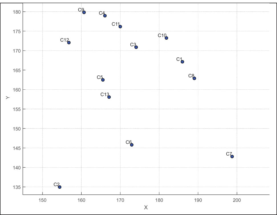
The coordinates of the elements in the logistics chain.

Figure 2

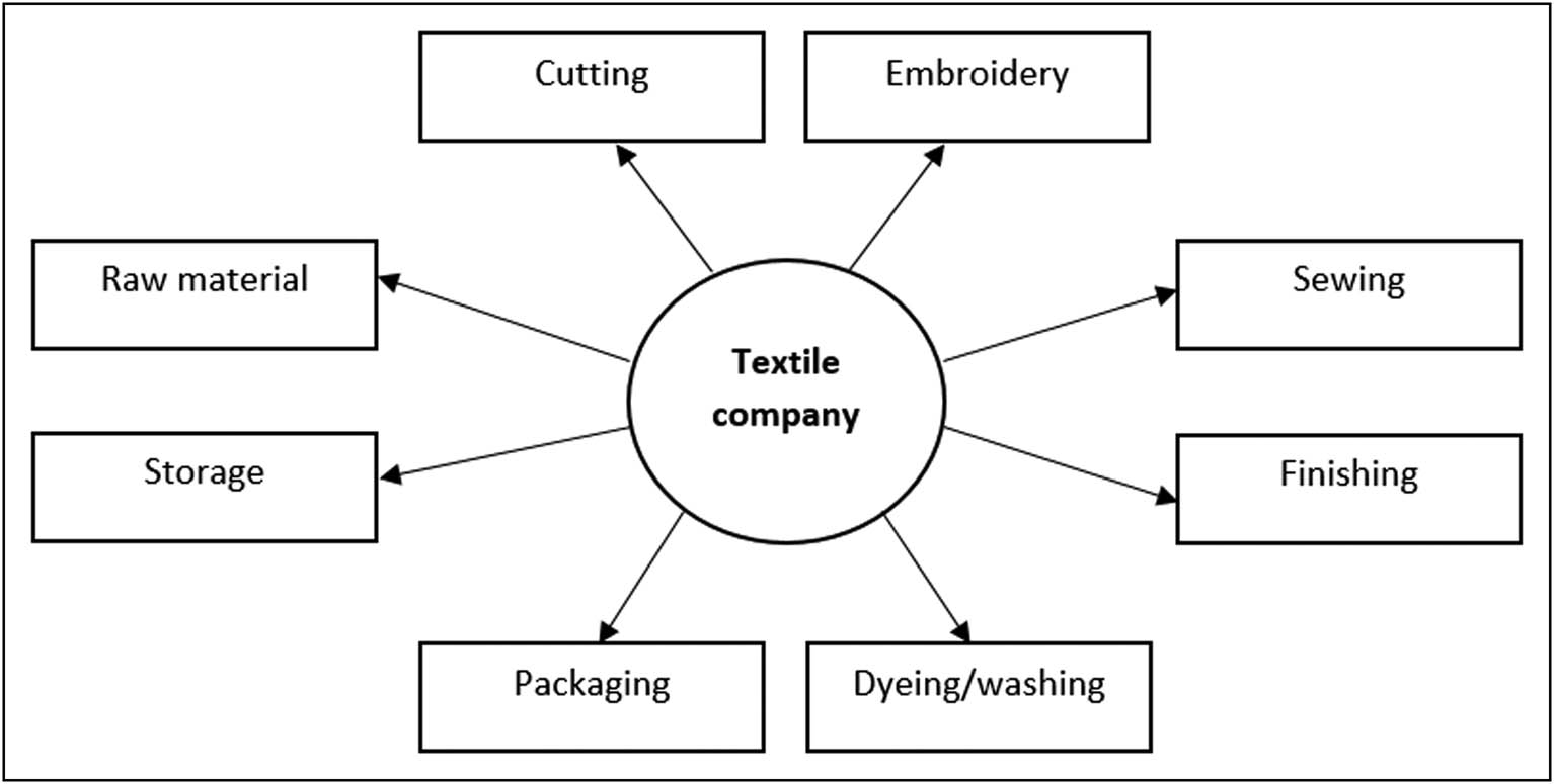
The phases of logistics within the textile industry.

2.3 ACO algorithm

2.3.1 Steps of the method

The ACO algorithm can be implemented using the following steps:

Initialization: Set parameters for the ACO algorithm, including pheromone evaporation rate, pheromone influence, and explorationexploitation balance. The initial pheromone levels will be set uniformly across all routes.
Pheromone updating rules: Develop rules for pheromone updating based on the routes selected by artificial ants. The pheromone levels will be reinforced when a route leads to a successful delivery (i.e., lower cost and timely delivery) and evaporates based on a predetermined rate to encourage exploration of new routes.
Heuristic function: Define a heuristic function that considers each route’s distance, transportation cost, and delivery time. The heuristic will guide the ants in selecting routes that minimize costs and optimize delivery times.
Ant movement simulation: Simulate the movement of virtual ants through the supply chain network. Based on the pheromone levels and heuristic function, each ant constructs a solution by moving from one node (e.g., supplier, manufacturer) to another.

2.3.2 Algorithm parameters

The following parameters were defined for the ACO algorithm:

Number of ants (N)
Number of iterations (T)
Pheromone importance (α)
Heuristic priority (β)
Evaporation rate (ρ)

2.3.3 Path construction

Each ant constructs a path based on the pheromone levels and distance. The probability of selecting the next city is determined using the following formula:

(1) P ij = ( τ ij ) α × ( µ ij ) β ∑ k ∈ allowed ( τ ik ) α × ( µ ik ) β ,

where τ ij is the pheromone level between city i and city j. µ ij is the heuristic information (inverse of distance, costs…). α and β control the influence of pheromones and heuristic information.

2.3.4 Pheromone update

After each iteration, pheromone levels are updated using the following formula:

(2) τ ij = ( 1 − ρ ) × τ ij + ∆ τ ij ,

where ρ is the pheromone evaporation rate.

(3) ∆ τ ij = Q L ,

where Q is a constant and L is the total length of the path taken by the ant.

2.4 Analytic Hierarchy Process (AHP) method

The AHP helps to categorize and make sense of decisions through a blend of principles and insights from psychology. The various calculation steps are as follows:

Step 1: The AHP method starts by identifying the options that need to be evaluated.

Step 2: Outlining the problem and establishing the criteria.

Step 3: Determining the importance of each criterion by comparing them in pairs.

Step 4: Ensuring that everything matches up correctly and stays on track consistently throughout the process.

Step 5: Figuring out the values to use in this situation.

3 Results

3.1 Optimizing driver scheduling

The company uses several drivers and transport facilities to perform all the functions and control the logistics chain. The logistics and transport planning manager is responsible for preparing the daily schedule for the drivers to cover different points in the supply chain, including subcontractors and other important points.

Table 2 presents all the parameters to be considered when creating a well-defined schedule for each driver. Key factors include distance to be travelled, estimated fuel consumption, road conditions, possible traffic delays, and the time required for visits at each subcontractor. We systematically list these elements in Table 2 to support informed decision-making and improve the planning process to maximize transportation efficiency throughout the supply chain.

Table 2

Optimization parameters for route analysis and cost evaluation

Index (l)	Optimization parameter (M _l)	Symbol
1	Distance matrix	DIS
2	Fuel consumption matrix	FUC
3	Traffic conditions matrix	TRC
4	Time spend matrix	TIS
5	Route conditions matrix	ROC
6	Fuel cost matrix	FCS
7	Maintenance cost matrix	MAC
8	Time cost matrix	TIC
9	Miscellaneous Fees matrix	MIF

3.2 Calculation of the matrix

To define and explain the problem more precisely, we will look at a specific schedule instance that consists of visiting several points. In this case, a plan was developed to visit seven locations: c1, c2, c3, c4, c5, c6, and c7. For this reason, it is necessary to calculate the distance between these points to determine the most effective way. Then, the required matrices for optimization and the best way to conduct the proposed visits were determined. This is because the approach will provide a clearer picture of the overall logistical complexities.

3.2.1 Distance matrix

The distance matrix includes distances between all relevant locations (e.g., suppliers, distribution centers, and customers). Table 3 shows an example matrix (in km).

Table 3

Distance matrix

	c1	c2	c3	c4	c5	c6	c7
c1	0.00	45.07	12.46	23.16	20.96	25.00	27.49
c2	45.07	0.00	40.94	45.51	29.68	21.47	45.04
c3	12.46	40.94	0.00	11.40	11.98	25.10	37.38
c4	23.16	45.51	11.40	0.00	16.49	33.87	48.76
c5	20.96	29.68	11.98	16.49	0.00	18.25	38.62
c6	25.00	21.47	25.10	33.87	18.25	0.00	25.99
c7	27.49	45.04	37.38	48.76	38.62	25.99	0.00

3.2.2 Fuel consumption matrix (in liters)

The values in this matrix represent the estimated fuel consumption for traveling between each pair of cities, as shown in Table 4. These estimates are calculated using the average fuel consumption rate of 6 L per 100 km. To determine the fuel consumption for each distance, the following formula is used:

(4) Fuel consumption = Distance 100 × 6 .

Table 4

Fuel consumption matrix

	c1	c2	c3	c4	c5	c6	c7
c1	0.00	2.70	0.75	1.39	1.26	1.50	1.65
c2	2.70	0.00	2.46	2.73	1.78	1.29	2.70
c3	0.75	2.46	0.00	0.68	0.72	1.51	2.24
c4	1.39	2.73	0.68	0.00	0.99	2.03	2.93
c5	1.26	1.78	0.72	0.99	0.00	1.10	2.32
c6	1.50	1.29	1.51	2.03	1.10	0.00	1.56
c7	1.65	2.70	2.24	2.93	2.32	1.56	0.00

3.2.3 Traffic matrix

The values are the traffic between each pair of cities on a scale of 0–1, where 0 is no traffic, and 1 is heavy traffic (Table 5). This information is important for determining delays and identifying better supply chain travel routes.

Table 5

Traffic matrix

	c1	c2	c3	c4	c5	c6	c7
c1	0.00	0.05	0.05	0.15	0.05	0.05	0.10
c2	0.05	0.00	0.05	0.10	0.05	0.05	0.05
c3	0.05	0.05	0.00	0.15	0.10	0.10	0.15
c4	0.15	0.10	0.15	0.00	0.20	0.15	0.25
c5	0.05	0.05	0.10	0.20	0.00	0.10	0.15
c6	0.05	0.05	0.10	0.15	0.10	0.00	0.10
c7	0.10	0.05	0.15	0.25	0.15	0.10	0.00

3.2.4 Time spent matrix

To create a time spent matrix based on the previous distance and traffic matrices, we can use the following formula:

(5) Time spent = Distance Average speed × ( 1 + Traffic level ) .

Assuming an average speed of 60 km/h for the calculations, we can derive the time spent in hours. Using the distances from the first matrix and the normalized traffic levels, we present the calculated time spent matrix in Table 6. This matrix will provide valuable insights into the expected travel times between each pair of cities, facilitating better scheduling and planning decisions within the supply chain.

Table 6

Time spent matrix

	c1	c2	c3	c4	c5	c6	c7
c1	0.00	0.79	0.22	0.44	0.37	0.44	0.50
c2	0.79	0.00	0.72	0.83	0.52	0.38	0.79
c3	0.22	0.72	0.00	0.22	0.22	0.46	0.72
c4	0.44	0.83	0.22	0.00	0.33	0.65	1.02
c5	0.37	0.52	0.22	0.33	0.00	0.33	0.74
c6	0.44	0.38	0.46	0.65	0.33	0.00	0.48
c7	0.50	0.79	0.72	1.02	0.74	0.48	0.00

3.2.5 Route condition matrix

The route condition matrix classifies the routes between the cities into three categories based on the route conditions.

0: In good condition (smooth and with good road surface).

0.02: Moderate condition (some potholes and moderate wear on the roads).

0.05: Poor condition (the roads are rough and wear significantly).

The matrix in Table 7 helps assess route suitability based on road conditions, which can impact travel time and vehicle performance. This is crucial for optimizing routes and planning in the supply chain network.

Table 7

Route condition matrix

	c1	c2	c3	c4	c5	c6	c7
c1	0	0.05	0.02	0.05	0.02	0.05	0.02
c2	0.05	0	0.05	0.02	0.05	0.05	0.05
c3	0.02	0.05	0	0.02	0.02	0.05	0.05
c4	0.05	0.02	0.02	0	0.02	0.05	0.02
c5	0.02	0.05	0.02	0.02	0	0.02	0
c6	0.05	0.05	0.05	0.05	0.02	0	0.05
c7	0.02	0.05	0.05	0.02	0	0.05	0

3.2.6 Fuel cost matrix

The fuel cost can be calculated using the following formula:

(6) Fuel cost = Fuel consumption × Price .

The matrix in Table 8 shows the estimated fuel costs of travelling between each pair of cities. In any case, they provide their results by combining fuel efficiency with the current fuel price to estimate costs for the entire transportation process. We can use these data to make more sophisticated fiscal decisions within the supply chain.

Table 8

Fuel cost matrix

	c1	c2	c3	c4	c5	c6	c7
c1	0.00	6.76	1.87	3.47	3.14	3.75	4.12
c2	6.76	0.00	6.14	6.83	4.45	3.22	6.76
c3	1.87	6.14	0.00	1.71	1.80	3.76	5.61
c4	3.47	6.83	1.71	0.00	2.47	5.08	7.31
c5	3.14	4.45	1.80	2.47	0.00	2.74	5.79
c6	3.75	3.22	3.76	5.08	2.74	0.00	3.90
c7	4.12	6.76	5.61	7.31	5.79	3.90	0.00

3.2.7 Maintenance costs

Costs incurred due to vehicle operation for maintenance include the following.

3.2.7.1 Normal maintenance costs

Standard maintenance is done after every 10,000 km, costing $100, which is $0.01 per km.

3.2.7.2 Replacement of tires costs

After reaching 100,000 km, these tires are changed for new ones, and they charge $400. Hence, it costs $0.004 per km.

3.2.7.3 Weighting factor

To account for variations in road conditions, we include a weighting factor for all model scenarios, which has a product of 0 for perfect conditions (no extra charge).

Roads requiring above-average maintenance costs are scaled up by 2% (0.02). Roads considered to be poor increase the cost by 5% in the model (0.05).

The total maintenance cost per kilometer for each pair of points (i, j) is given by the formula:

(7) Maintenance Cost per km i → j = C × ( 1 + Weig h ting Factor i → j ) .

This calculation determines the total transportation costs. The results are displayed in Table 9, which shows the maintenance cost matrix for the distance between cities. This information is crucial for adequately controlling costs in the supply chain.

Table 9

Maintenance cost matrix

	c1	c2	c3	c4	c5	c6	c7
c1	0.00	0.66	0.18	0.34	0.30	0.37	0.39
c2	0.66	0.00	0.60	0.65	0.44	0.32	0.66
c3	0.18	0.60	0.00	0.16	0.17	0.37	0.55
c4	0.34	0.65	0.16	0.00	0.24	0.50	0.70
c5	0.30	0.44	0.17	0.24	0.00	0.26	0.54
c6	0.37	0.32	0.37	0.50	0.26	0.00	0.38
c7	0.39	0.66	0.55	0.70	0.54	0.38	0.00

3.2.8 Time costs

Time costs represent the economic value of the time spent traveling, including the hourly wage of the driver and any assistants involved in the transportation process. The formula for calculating time costs is

(8) Time cost = Time spent × Hourly wage of the driver .

This calculation helps understand the overall transportation costs, and the results are shown in Table 10. This table is useful for making informed financial decisions within the supply chain.

Table 10

Time cost matrix

	c1	c2	c3	c4	c5	c6	c7
c1	0.00	3.94	1.09	2.22	1.83	2.19	2.52
c2	3.94	0.00	3.58	4.17	2.60	1.88	3.94
c3	1.09	3.58	0.00	1.09	1.10	2.30	3.58
c4	2.22	4.17	1.09	0.00	1.65	3.25	5.08
c5	1.83	2.60	1.10	1.65	0.00	1.67	3.70
c6	2.19	1.88	2.30	3.25	1.67	0.00	2.38
c7	2.52	3.94	3.58	5.08	3.70	2.38	0.00

3.2.9 Miscellaneous fees

This matrix presented in Table 11 is a framework for identifying and estimating additional fees during transportation. Costs can be estimated to fit certain operations and market conditions. They may include tolls for using toll roads, parking fees charged at delivery points, and all charges relating to the loading and unloading of the goods. These costs only needed to be adjusted to give a better picture of the possible costs.

Table 11

Miscellaneous fees matrix

	c1	c2	c3	c4	c5	c6	c7
c1	0	2	1.75	2.25	2.5	2.1	1.9
c2	2	0	2.2	1.7	2.4	2	2.15
c3	1.75	2.2	0	2	1.85	2.05	2.25
c4	2.25	1.7	2	0	2.1	1.8	2.3
c5	2.5	2.4	1.85	2.1	0	2.2	1.95
c6	2.1	2	2.05	1.8	2.2	0	2
c7	1.9	2.15	2.25	2.3	1.95	2	0

Table 11 shows a miscellaneous fees matrix showing the fees for each route between locations c1 and c7. It also includes the cost of permits, tolls, or any other incidental expenditures.

3.3 Human decision-making in route assignment for drivers

After evaluating all the matrices, the logistics manager, based on their expertise, decides which driver takes which route. This decision, shown in Figure 3, indicates the paths drivers should take during the planned visits.

Figure 3

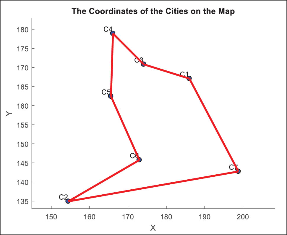
Recommended driver route for planned visits.

Table 12 details the breakdown of the total costs incurred in travelling from one city to another. This analysis is based on the decisions of the logistics manager who set the planning policy. As for the total transportation cost, we get 53.04 for the specified route. The total cost includes other expenses, such as time costs, which are often the hourly salary of the driver, maintenance expenses, and fuel expenses.

Table 12

Final cost calculation by human decision-maker

	C1	C2	C3	C4	C5	C6	C7
C1	0.00	13.37	4.89	8.29	7.78	8.41	8.94
C2	13.37	0.00	12.53	13.35	9.89	7.41	13.51
C3	4.89	12.53	0.00	4.96	4.92	8.48	11.99
C4	8.29	13.35	4.96	0.00	6.46	10.62	15.39
C5	7.78	9.89	4.92	6.46	0.00	6.87	11.98
C6	8.41	7.41	8.48	10.62	6.87	0.00	8.66
C7	8.94	13.51	11.99	15.39	11.98	8.66	0.00

3.4 Application of the ant colony algorithm

The probability P _ij of moving from city i to city j can be formulated to consider various parameters as follows:

(9) P ij = ( τ ij ) α × ( µ ij ) β ∑ k ∈ N j ( τ ik ) α × ( µ ik ) β .

3.4.1 Ant colony algorithm parameters

Set the parameters needed for the ACO algorithm as follows:

Number of ants ( N ): Set to 10.
Number of iterations ( T ): Set to 100.
Pheromone importance ( α ): Set to 0.5.
Heuristic importance ( β ): Set to 2.
Evaporation rate ( ρ ): Set to 0.5.
Constant ( Q ): Set to 100 (this can be adjusted based on the scale of the problem).

3.4.2 Defining the composite function µ ij

The composite function μ ij can be defined to incorporate various parameters

(10) µ ij = ∑ l = 1 9 w l × 1 M l , ij ,

where w l is the weights representing the importance of each parameter in the optimization process. M l , ij is the lth optimization parameter between city i and j.

3.4.3 Assigning weights to matrices using the AHP method

In our study, the AHP approach is used to assign the weight of each parameter. Table 13 presents the pairwise comparison matrix between the criteria.

Table 13

Pairwise comparison matrix of criterion

	DIS	FUC	TRC	TIS	ROC	FCS	MAC	TIC	MIF
DIS	1.00	2.00	3.00	3.00	2.00	2.00	3.00	2.00	3.00
FUC	0.50	1.00	2.00	0.50	2.00	2.00	2.00	2.00	2.00
TRC	0.33	0.50	1.00	0.50	0.50	0.50	2.00	2.00	2.00
TIS	0.33	2.00	2.00	1.00	0.50	0.50	2.00	0.50	2.00
ROC	0.50	0.50	2.00	2.00	1.00	0.50	0.50	0.50	2.00
FCS	0.50	0.50	2.00	2.00	2.00	1.00	0.50	2.00	2.00
MAC	0.33	0.50	0.50	0.50	2.00	2.00	1.00	0.50	2.00
TIC	0.50	0.50	0.50	2.00	2.00	0.50	2.00	1.00	2.00
MIF	0.50	0.50	0.50	0.50	0.50	0.50	0.50	0.50	1.00

Table 14 presents the normalization matrix. We also calculate the consistency ratio, as shown in Table 15.

Table 14

Normalization matrix

	DIS	FUC	TRC	TIS	ROC	FCS	MAC	TIC	MIF	Weight	Consistency
DIS	0.22	0.25	0.22	0.25	0.16	0.21	0.22	0.18	0.17	0.21	10.15
FUC	0.11	0.13	0.15	0.04	0.16	0.21	0.15	0.18	0.11	0.14	10.10
TRC	0.07	0.06	0.07	0.04	0.04	0.05	0.15	0.18	0.11	0.09	10.10
TIS	0.07	0.25	0.15	0.08	0.04	0.05	0.15	0.05	0.11	0.11	10.12
ROC	0.11	0.06	0.15	0.17	0.08	0.05	0.04	0.05	0.11	0.09	10.11
FCS	0.11	0.06	0.15	0.17	0.16	0.11	0.04	0.18	0.11	0.12	10.15
MAC	0.07	0.06	0.04	0.04	0.16	0.21	0.07	0.05	0.11	0.09	10.00
TIC	0.11	0.06	0.04	0.17	0.16	0.05	0.15	0.09	0.11	0.10	10.18
MIF	0.11	0.06	0.04	0.04	0.04	0.05	0.04	0.05	0.06	0.05	9.81

Table 15

Consistency ratio

RI	1.45
n	9.00
γ max	10.08
CI	0.14
CR	0.09

We finalize and validate the AHP method results following a complete mathematical approach. The most crucial criticism we seek to determine is the consistency ratio (CR)

(11) CR = CI RI ,

where RI is the random index presented in Table 16. CI is the consistency index determined using the following formula:

(12) CI = γ max − n n − 1 ,

where n is the order of the matrix. γ max is the average of all the consistency values.

Table 16

Random index (RI)

n	1	2	3	4	5	6	7	8	9	10
RI	0	0	0.58	0.90	1.12	1.24	1.32	1.41	1.45	1.49

3.4.3.1 Derive an overall relative score for each alternative

According to the AHP method, the weights for each parameter are presented in Table 17.

Table 17

Normalization matrix

Parameters	Weights
Distance (DIS)	0.21
Fuel consumption (FUC)	0.14
Traffic (TRC)	0.09
Time spent (TIS)	0.11
Route conditions (ROC)	0.09
Fuel costs (FCS)	0.12
Maintenance costs (MAC)	0.09
Time costs (TIC)	0.10
Miscellaneous fees (MIF)	0.05

3.4.4 Results of ACO

The ACO program has processed all the data in the matrices, which are very important in calculating transportation cost optimization. The program devised a route to visit the seven points by considering the different weights of the matrices and using the right optimization techniques. Therefore, the ACO algorithm provided an optimal path, as shown in Figure 4.

Figure 4

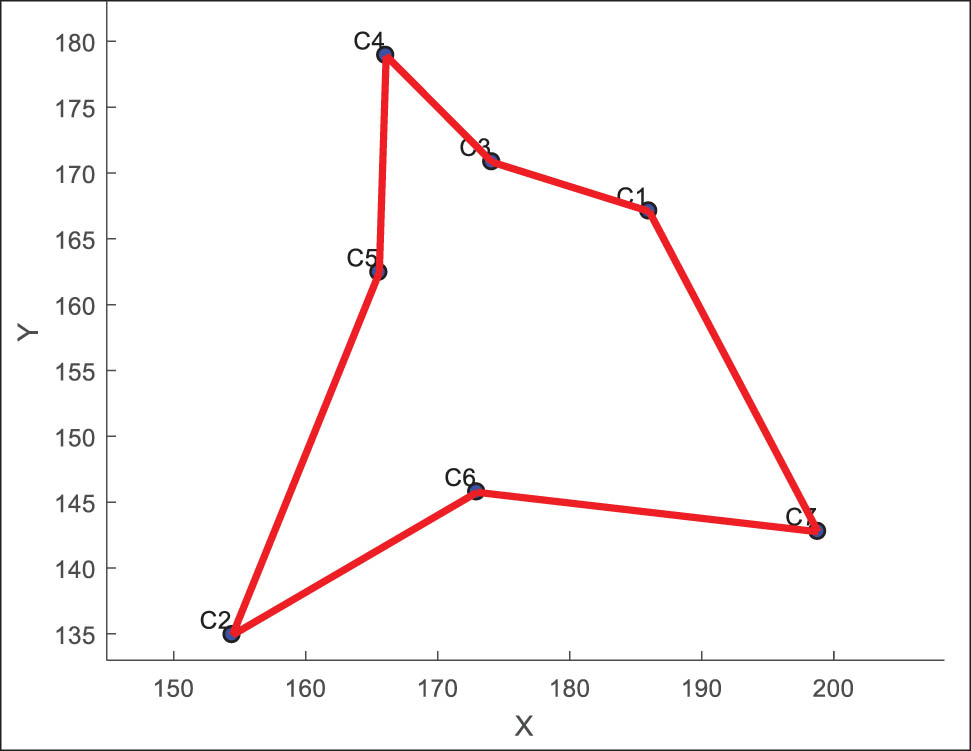
Route selected by the ant colony algorithm.

By adopting the route selected by the Ant Colony algorithm and considering all the given parameters, we present the final calculations of various costs in Table 18, along with the total cost for each transition between points. All these data are summarized in Table 18.

Table 18

Final cost calculation by Ant Colony program (in $)

	From	To	Total cost	Fuel cost	Maintenance cost	Time cost	Miscellaneous cost
Segment 1	1	7	8.93	4.12	0.39	2.52	1.90
Segment 2	7	6	8.66	3.90	0.38	2.38	2.00
Segment 3	6	2	7.42	3.22	0.32	1.88	2.00
Segment 4	2	5	9.89	4.45	0.44	2.60	2.40
Segment 5	5	4	6.46	2.47	0.24	1.65	2.10
Segment 6	4	3	4.96	1.71	0.16	1.09	2.00
Segment 7	3	1	4.89	1.87	0.18	1.09	1.75
Total			51.21	21.74	2.11	13.21	14.15

Based on the previous table, we can conclude that the route discovered by the ACO program has a total transportation cost of 51.21$, which is incurred through four significant components: Fuel cost (21.74), maintenance cost (2.11), time cost (13.21), and miscellaneous cost (14.15).

4 Discussion

To confirm and strengthen the results obtained above, several factors, including the convergence graph, the pheromone concentration heatmap, and the generalized cost for additional cases, must be checked and presented.

4.1 Convergence graph

The convergence graph is a visual representation that illustrates how the solution quality (in terms of cost) improves over the iterations of the ACO algorithm. The primary purpose of the convergence graph is to show the progress of the optimization process.

In Figure 5, we plotted the convergence graph of the ACO algorithm, which effectively contains two distinct parameters. The first parameter, which is positioned on the horizontal axis, covers the number of iterations performed by the algorithm. In contrast, the second parameter, cost, with the best-identified solution, is the suggested unit on the vertical axis. This cost parameter may cover distance, fuel, time, and maintenance in line with the problems under consideration.

Figure 5

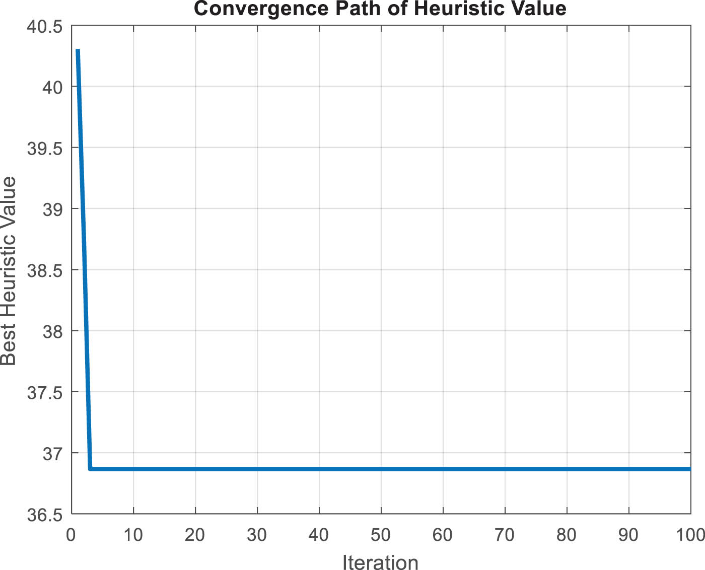
Convergence graph.

The graph is expected to dip, meaning that the best cost found improves with each iteration (time). This implies that the solution is being well explored and is moving toward an optimum result. It is also customary to observe plateaus, where the cost remains constant for several iterations. This means the algorithm is doing all right but is not venturing out significantly from the original paths.

The last cost graph shows the algorithm’s best solution, which is the best or reasonably best cost accomplished while using the ACO. The convergence graph gives practitioners the means to evaluate the efficiency and effectiveness of the ACO algorithm.

4.2 Pheromone level heatmap

The pheromone level heatmap is a graph that shows the pheromone levels of different paths in the ACO algorithm, highlighting their importance. In ACO, pheromones are used as a form of communication between artificial ants, where each ant deposits pheromones on the paths it follows, which in turn influences other ants to choose those paths in subsequent iterations. The concentration of pheromones along a path indicates its quality based on costs related to distance and fuel consumption; higher levels signal routes frequently traveled by many ants in the past. This heatmap not only displays the pheromone density in the paths of the search space but also helps show how the ants learn from each other to reach optimal solutions.

The pheromone level heatmap in Figure 6 is a 2D graphical representation where the x-axis typically represents destination locations, and the y-axis represents starting locations. The color intensity in each cell corresponds to the pheromone levels of the path between these points, with darker colors indicating higher levels of pheromones, which are paths preferred by ants because they are associated with lower costs or better performance, and lighter colors indicating less attractive paths that might be longer or less efficient. Pheromone levels are dynamically updated as the ACO algorithm progresses by the paths chosen by the ants, and the result is a heatmap that evolves and shows the collective learning of the ant colony on this. This heatmap helps determine the convergence towards optimal algorithm solutions, assess the pheromone updating strategy, and explore the paths.

Figure 6

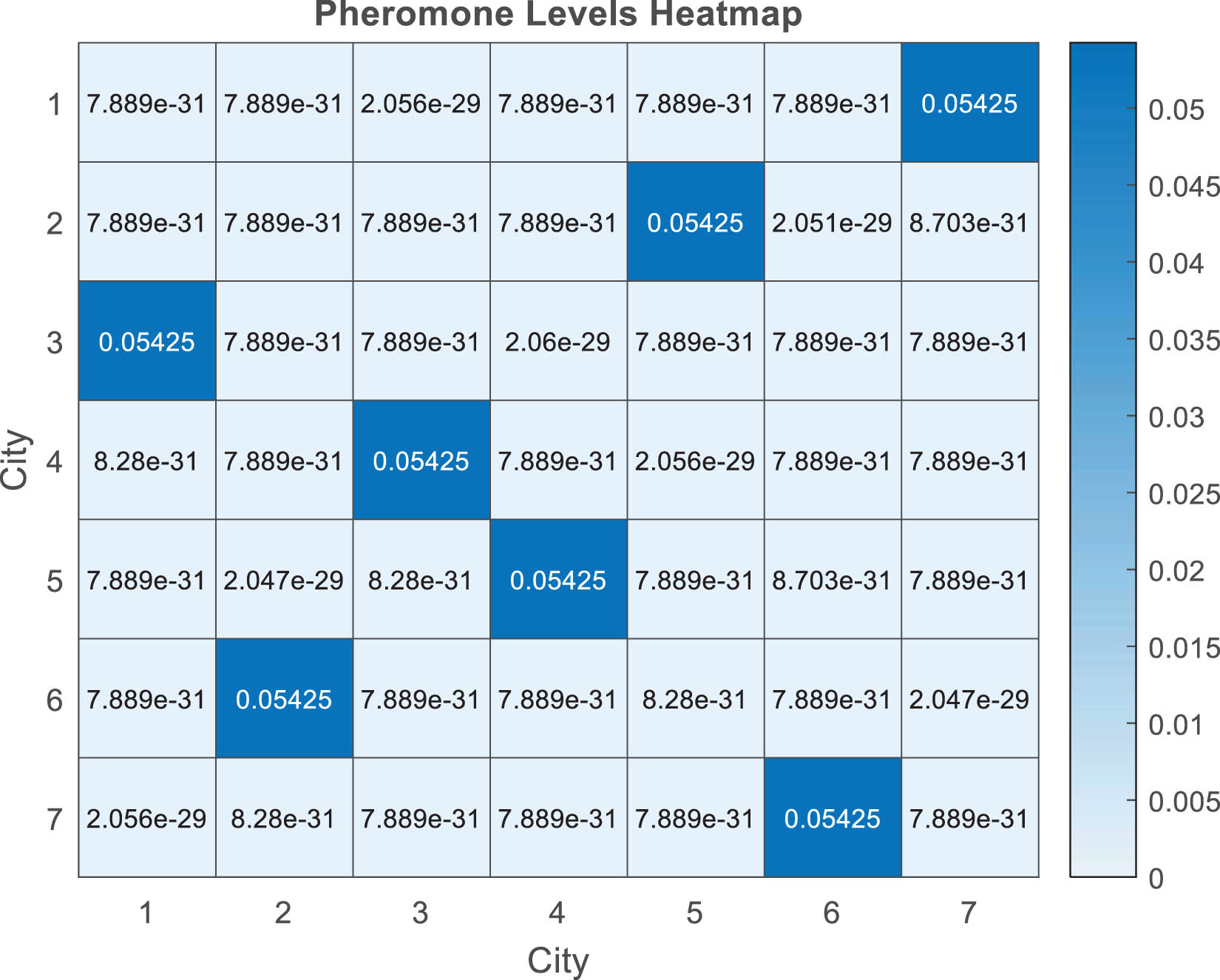
Pheromone level heatmap.

4.3 Model validation through calculated generalization

In this section, we will use a database of planning data as presented in Table 19 to test our calculation model using the Ant Colony algorithm. We will incorporate decisions made by logistics managers and compare the planning results based on the distance travelled by drivers and the total cost of allocation.

Table 19

Planning data

	P1	P2	P3	P4	P5
c1	✓	✓	✓	✓	✓
c2	✓	✓	✓		✓
c3	✓		✓		✓
c4	✓	✓		✓	✓
c5		✓			✓
c6	✓				✓
c7	✓	✓	✓	✓	✓
c8		✓	✓	✓
c9	✓		✓	✓
c10		✓	✓	✓
c11	✓	✓	✓	✓	✓
c12	✓	✓	✓	✓	✓
c13	✓	✓	✓	✓	✓

Table 20 compares two planning strategies, ACO and human decision-making, across five programs (P1–P5). Each program identifies the paths taken, the total costs incurred, and the distances travelled, with each row representing a different program using these two methods. The “Chosen Path” column defines the sequence of locations (c1, c2, etc.) visited and how they differ for the ACO and human decision sections. The “Total Cost” column presents the costs incurred for each path, and lower costs indicate better planning. At the same time, the “Distance Travelled” column shows the total distance covered, and fewer distances are generally more effective in route planning.

Table 20

Comparison of ACO and human decision-making

Program	Planning by	Chosen path	Total cost ($)	Distance travelled (km)
P1	Ant Colony program	c1-c3-c11-c4-c9-c12-c13-c2-c6-c7-c1	60.35	156.82
P1	Human decision	c1-c7-c6-c13-c2-c12-c9-c4-c3-c11-c1	71.71	181.16
P2	Ant Colony program	c1-c10-c11-c4-c12-c5-c13-c2-c7-c8-c1	56.13	152.59
P2	Human decision	c1-c10-c4-c11-c5-c12-c13-c2-c7-c8-c1	62.26	172.74
P3	Ant Colony program	c1-c10-c3-c11-c9-c12-c13-c2-c7-c8-c1	59.61	157.22
P3	Human decision	c1-c3-c10-c11-c9-c13-c12-c2-c7-c8-c1	67.14	192.67
P4	Ant Colony program	c1-c10-c11-c4-c9-c12-c13-c7-c8-c1	46.59	118.61
P4	Human decision	c1-c11-c10-c4-c9-c12-c7-c13-c8-c1	65.80	175.51
P5	Ant Colony program	c1-c3-c11-c4-c12-c5-c13-c6-c2-c7-c1	61.35	160.78
P5	Human decision	c1-c5-c3-c11-c4-c12-c2-c13-c6-c7-c1	71.63	186.64

The Ant Colony programs are generally better at minimizing total cost than human decisions across all five programs. Mostly, the distances travelled using Ant Colony methods are shorter than those of human decisions, which further supports their efficiency. In P4, the ACO path costs 46.59$ and covers a 118.61 km distance, while the human decision method costs 65.80$ and covers a 175.51 km distance, thus demonstrating a significant advantage for ACO. However, the consistent performance of the ACO algorithm suggests that there may be certain conditions under which human decision-making can be as good as, or even better than, the ACO algorithm. In conclusion, the ACO algorithm is generally more cost-effective and offers better convergence in terms of path length compared to human heuristics. The findings of our study show striking similarities with outcomes acquired from different studies within the same field of study. This similarity suggests that the outcomes we reached are consistent with observations made by other scholars, thereby strengthening the validity of our findings [36,37,38]. Therefore, it could be a valuable tool for various problems. A more detailed analysis might examine when and why the paths and costs differ and what this means in practice.

Table 21 summarizes the combined costs and the corresponding distances of the two methods, i.e., ACO with human decisions, highlighting their differences.

Table 21

Descriptive statistics

Metric	ACO	Human decisions
Mean (total cost)	60.81	67.51
Median (total cost)	59.61	67.14
Std. dev. (total cost)	5.86	3.87
Mean (distance)	149.84	181.14
Median (distance)	157.22	181.16
Std. dev. (distance)	17.51	7.76

Figures 7 and 8 compare the cost value and distance shifts of the Ant Colony algorithm and human decision-makers. Figure 7 shows that the Ant Colony algorithm generally incurs lower travel costs as it explores multiple routes simultaneously and selects the best option in real-time.

Figure 7

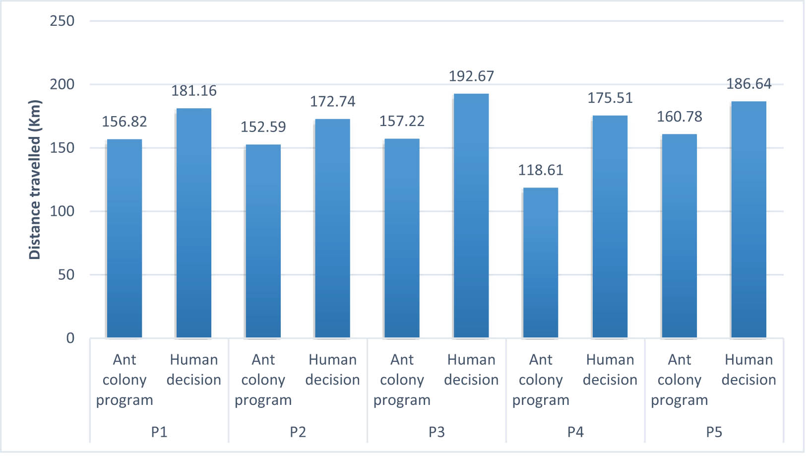
Comparison of the ant colony algorithm and human decision-making in terms of distance travelled.

Figure 8

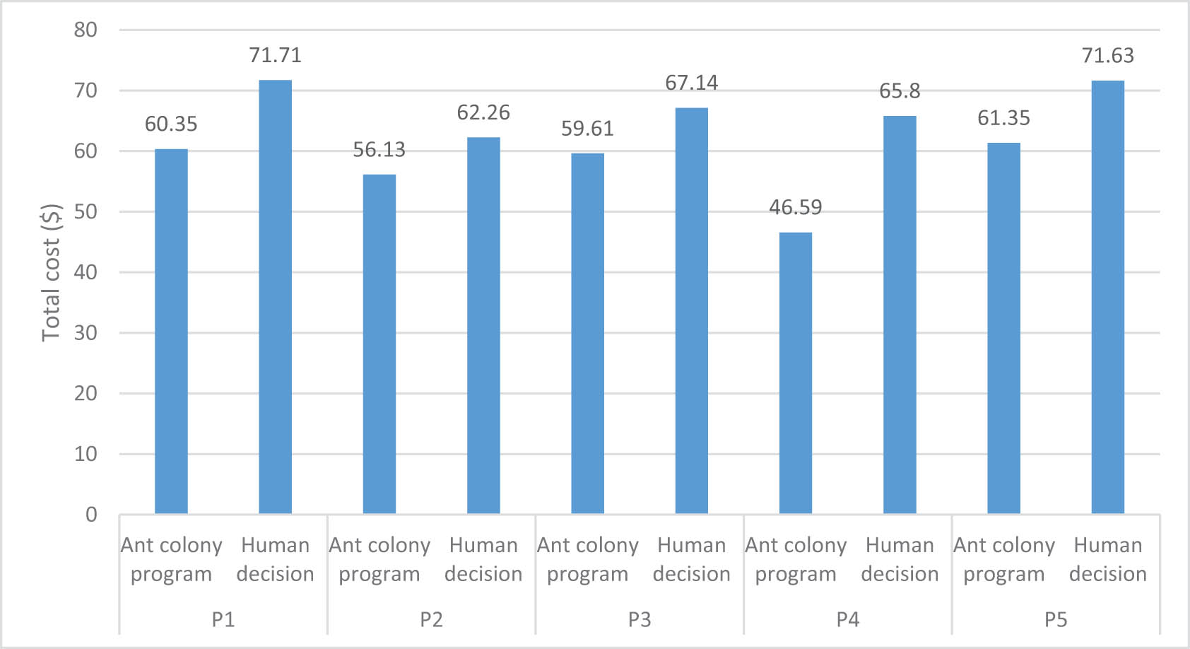
Comparison of the ant colony algorithm and human decision-making in terms of cost value.

In other words, people’s travel distances and costs are higher than the algorithm. Figure 8 shows costs incurred by transports of varying distances, and the ant algorithm has also shown lower costs. This method results in fewer travel kilometers with effective logistical measures. The figures highlight the effectiveness of decision-support systems that use algorithms in logistics, offering required services in the most cost-efficient way.

To effectively reconcile the different criteria such as distance, cost, fuel consumption, and traffic, we proposed using the AHP method. This approach allowed us to establish a scientific balance between the criteria identified in our study, prioritizing them according to their relative importance. In addition, the answer to the problem of choosing several criteria was found when applying the probability function integrated into the ant colony algorithm. This multi-criteria function grouped and evaluated the different parameters studied, thus providing a coherent and optimized solution that considered all the essential aspects. By combining the AHP method with the ant colony algorithm, we developed a robust and efficient optimization model, capable of addressing the complex challenges of the textile supply chain.

5 Conclusion

The use of ACO in transportation logistics for the textile industry supply chain is unique in that it attempts to solve specific significant problems in the transportation sector. ACO successfully solves complicated logistical problems involving several distribution centers by mimicking the actions of ants, who consider distance, fuel use, expenses, and even time-sensitive deliveries. This study outlines the key aspects of ACO, focusing on the pheromone updating rules and the decision-making processes of virtual ants, which help to identify the best routing problem solutions. The integration of the ACO model has significantly improved transportation performance and service levels in the textile industry using a combination of computer modeling and case studies. The results indicate that the ACO model leads to cost savings and enhances operational flexibility and sustainability in logistics. Given the growing challenges in SCM, such as reducing the carbon footprint, ACO improves its competitive edge by increasing operational efficiency.

We would like to emphasize that all the research objectives stated at the beginning of our article have been achieved and successfully completed. In particular, we have succeeded in developing a robust model based on the optimization of several criteria, allowing us to obtain calculations aimed at optimizing both transport costs and distances.

In conclusion, using ACO in SCM gives the textile sector a potential solution to several challenges in modern logistics. With the new optimization, businesses can better meet the demands of changing environments and emerging markets, leading to a positive and stronger business position. By incorporating the AHP and ACO algorithms in a novel manner, our study greatly aids the academic and research communities by providing new perspectives on SCM within the textile sector. This research builds upon existing logistics theory and provides working models of practical value, fosters collaboration across domains, and strengthens the structure of subsequent studies. Moreover, these findings may be useful as yardsticks for the methodologies and metrics in other identical studies.

Acknowledgments

Princess Nourah bint Abdulrahman University Researchers Supporting Project number (PNURSP2025R246), Princess Nourah bint Abdulrahman University, Riyadh, Saudi Arabia.

Funding information: The research was financially supported by Princess Nourah bint Abdulrahman University Researchers Supporting Project number (PNURSP2025R246), Princess Nourah bint Abdulrahman University, Riyadh, Saudi Arabia.
Author contributions: All authors accepted responsibility for the entire content of this manuscript, consented to its submission to the journal, reviewed all results, and approved the final version of the manuscript. Mourad Lahdhiri, Mohamed Jmali, Thouraya Hamdi, and Amel Babay contributed to the writing, review, investigation, analysis, and validation of the manuscript. Mourad Lahdhiri, Mohamed Jmali, and Thouraya Hamdi developed the models.
Conflict of interest: The authors state no conflict of interest.
Ethical approval: The conducted research is not related to either human or animal use.
Data availability statement: The datasets generated during and/or analysed during the current study are available from the corresponding author on reasonable request.

References

[1] Staritz, C., Plank, L., Morris, M. (2016). Global value chains, industrial policy, and sustainable development–Ethiopia’s apparel export sector. Country Case Study. International Centre for Trade and Sustainable Development (ICTSD), Geneva.Search in Google Scholar

[2] Kumar, P., Sharma, D., Pandey, P. (2023). Coordination mechanisms for digital and sustainable textile supply chain. International Journal of Productivity and Performance Management, 72(6), 1533–1559.10.1108/IJPPM-11-2020-0615Search in Google Scholar

[3] Nakandala, D., Samaranayake, P., Lau, H. C. (2013). A fuzzy-based decision support model for monitoring on-time delivery performance: A textile industry case study. European Journal of Operational Research, 225(3), 507–517.10.1016/j.ejor.2012.10.010Search in Google Scholar

[4] Muckstadt, J. A., Murray, D. H., Rappold, J. A., Collins, D. E. (2001). Guidelines for collaborative supply chain system design and operation. Information Systems Frontiers, 3, 427–453.10.1023/A:1012824820895Search in Google Scholar

[5] Siddaramu, S. M., Ramaswamy, R. K. (2025). Optimal wireless sensor network ant-lifetime routing algorithm using multi-phase pheromone. Ingénierie des Systèmes d’Information, 30(1), 83.10.18280/isi.300108Search in Google Scholar

[6] Chaudhry, H., Hodge, G. (2012). Postponement and supply chain structure: cases from the textile and apparel industry. Journal of Fashion Marketing and Management: An International Journal, 16(1), 64–80.10.1108/13612021211203032Search in Google Scholar

[7] Abdulghani, B. A., Abdulghani, M. A. (2024). A comprehensive review of Ant Colony Optimization in swarm intelligence for complex problem solving. Acadlore Transactions on Machine Learning, 3(4), 214–224.10.56578/ataiml030403Search in Google Scholar

[8] Ma, K., Thomassey, S., Zeng, X. (2020). Development of a central order processing system for optimizing demand-driven textile supply chains: A real case based simulation study. Annals of Operations Research, 291(1), 627–656.10.1007/s10479-018-3000-2Search in Google Scholar

[9] Agrawal, T. K., Kumar, V., Pal, R., Wang, L., Chen, Y. (2021). Blockchain-based framework for supply chain traceability: A case example of textile and clothing industry. Computers & Industrial Engineering, 154, 107130.10.1016/j.cie.2021.107130Search in Google Scholar

[10] Dzalbs, I., Kalganova, T. (2020). Accelerating supply chains with Ant Colony Optimization across a range of hardware solutions. International Journal of Computer Applications, 176(15), 23–30.10.1016/j.cie.2020.106610Search in Google Scholar PubMed PubMed Central

[11] Moparthi, R. (2016). Speed optimized implementation of Ant Colony Optimization algorithm for image edge detection. International Journal of Computer Science and Information Security, 14(10), 791–796.Search in Google Scholar

[12] Philippe, L., Christian, P., Alain, T. (2022). First Competitive ant colony scheme for the CARP. Computers and Operations Research, 122, 104941.Search in Google Scholar

[13] Haryanto, W., Kusnadi, A., Soelistio, E. (2015). Warehouse layout method based on ant colony and backtracking algorithm. Journal of Physics: Conference Series, 655, 012070.Search in Google Scholar

[14] Tan, F., Lee, S., Majid, A., Seow, V. (2012). Ant colony optimization for capacitated vehicle routing problem. International Journal of Mathematical Models and Methods in Applied Sciences, 6(5), 869–876.Search in Google Scholar

[15] Pellonperä, T. (2014). Ant colony optimization and the vehicle routing problem. Journal of Transportation Engineering, 140(9), 04014059.Search in Google Scholar

[16] Yap, C., Lee, S., Majid, A., Seow, V. (2012). Ant colony optimization for container loading problem. Journal of Industrial Engineering and Management, 5(4), 836–854.Search in Google Scholar

[17] Liu, R., Yang, Y. (2013). The location-routing problem of urban disaster emergency based on an improved ant colony algorithm. Journal of Computers, 8(5), 1249–1256.10.4304/jcp.8.4.968-974Search in Google Scholar

[18] Flórez, E., Gómez, W., Bautista, L. (2019). An ant colony optimization algorithm for job shop scheduling problem. Applied Mathematical Modelling, 73, 804–818.Search in Google Scholar

[19] De Santis, R., Montanari, R., Vignali, G., Bottani, E. (2018). An adapted ant colony optimization algorithm for the minimization of the travel distance of pickers in manual warehouses. Journal of Manufacturing Science and Engineering, 140(7), 071008.Search in Google Scholar

[20] Narasimha, K. V., Kivelevitch, E., Sharma, B., Kumar, M. (2013). An ant colony optimization technique for solving min–max multi-depot vehicle routing problem. Swarm and Evolutionary Computation, 13, 63–73.10.1016/j.swevo.2013.05.005Search in Google Scholar

[21] Wang, X., Choi, T. M., Liu, H., Yue, X. (2016). Novel ant colony optimization methods for simplifying solution construction in vehicle routing problems. IEEE Transactions on Intelligent Transportation Systems, 17(11), 3132–3141.10.1109/TITS.2016.2542264Search in Google Scholar

[22] Yue, L. (2023, September). Sustainable supply chain distribution model of fashion market based on improved ant colony algorithm. In 2023 International Conference on Industrial IoT, Big Data and Supply Chain (IIoTBDSC) (pp. 289–293). IEEE.10.1109/IIoTBDSC60298.2023.00058Search in Google Scholar

[23] Sakalli, U. S. (2018). Ant colony optimization and genetic algorithm for fuzzy stochastic production-distribution planning. Applied Sciences, 8(11), 2042.10.3390/app8112042Search in Google Scholar

[24] Guan, X. (2023). Optimization of cold chain logistics vehicle transportation and distribution model based on improved ant colony algorithm. Procedia Computer Science, 228, 974–982.10.1016/j.procs.2023.11.128Search in Google Scholar

[25] Chen, S., Zheng, Y., Cattani, C., Wang, W. (2012). Modeling of biological intelligence for SCM system optimization. Computational and Mathematical Methods in Medicine, 2012(1), 769702.10.1155/2012/769702Search in Google Scholar PubMed PubMed Central

[26] Hfeda, M. (2018). Supply chain management optimization using meta-heuristics approaches applied to a case in the automobile industry. Procedia CIRP, 72, 447–452.Search in Google Scholar

[27] Kazemi, A., Kangi, F., Amiri, M. (2013). Meta-heuristic algorithms for an integrated production-distribution planning problem in a multi-objective supply chain. International Journal of Advanced Manufacturing Technology, 67(9), 2315–2326.Search in Google Scholar

[28] Wang, C. N., Pham, T. D. T., Nhieu, N. L. (2021). Multi-layer fuzzy sustainable decision approach for outsourcing manufacturer selection in apparel and textile supply chain. Axioms, 10(4), 262.10.3390/axioms10040262Search in Google Scholar

[29] Ghasemy Yaghin, R. (2022). Textile supply chain management considering carbon emissions and apparel demand fuzziness: a fuzzy mathematical programming approach. International Journal of Clothing Science and Technology, 34(2), 137–155.10.1108/IJCST-08-2020-0124Search in Google Scholar

[30] Guo, F. (2017). On production and green transportation coordination in a sustainable global supply chain. Sustainability, 9(11), 2071.10.3390/su9112071Search in Google Scholar

[31] Jafari, H. R. (2017). Sustainable supply chain design with water environmental impacts and justice-oriented employment considerations: A case study in textile industry. Scientia Iranica, 24(4), 2119–2137.10.24200/sci.2017.4299Search in Google Scholar

[32] Andreica, M. (2009). Algorithmic solutions to some transportation optimization problems with applications in the metallurgical industry. Romanian Journal of Economic Forecasting, 12(3), 91–104.Search in Google Scholar

[33] Liu, Y. (2024). Modelling of optimal transportation route selection based on artificial bee colony algorithm. Journal of Transportation Engineering, 150(1), 04023015.10.1504/IJGEI.2023.10056904Search in Google Scholar

[34] Berthier, C. (2020). Case study of supply chain in textile industry: A dynamic product allocation decision problem. International Journal of Production Economics, 220, 107454.Search in Google Scholar

[35] Olivares-Benitez, J. (2013). A metaheuristic algorithm to solve the selection of transportation channels in supply chain design. Computers & Industrial Engineering, 64(2), 474–482.Search in Google Scholar

[36] Hoa, N. T. X. (2024, February). Applying ant colony optimization for inventory routing problem to improve the performance in distribution chain: A case study of Vietnamese garment company. In 11th International Conference on Emerging Challenges: Smart Business and Digital Economy 2023 (ICECH 2023) (pp. 565–578). Atlantis Press.10.2991/978-94-6463-348-1_44Search in Google Scholar

[37] Messaoud, A. (2024). A hybrid ant colony optimization algorithm to solve a transport problem with stochastic customer demands and electric vehicles of limited load capacity. Transportation Research Part E: Logistics and Transportation Review, 165, 102868.10.1007/s12065-023-00901-8Search in Google Scholar

[38] Wu, Y. (2024). A multi-objective ant colony system-based approach to transit route network adjustment. Transportation Research Part B: Methodological, 158, 189–205.10.1109/TITS.2023.3348111Search in Google Scholar

Received: 2025-03-15

Revised: 2025-06-09

Accepted: 2025-09-24

Published Online: 2025-11-06

This work is licensed under the Creative Commons Attribution 4.0 International License.

Articles in the same Issue

https://doi.org/10.1515/aut-2025-0058

Keywords for this article

Ant colony optimization; supply chain management; textile industry; transport optimization; logistics efficiency

Creative Commons

BY 4.0

	P1	P2	P3	P4	P5
c1	✓	✓	✓	✓	✓
c2	✓	✓	✓		✓
c3	✓		✓		✓
c4	✓	✓		✓	✓
c5		✓			✓
c6	✓				✓
c7	✓	✓	✓	✓	✓
c8		✓	✓	✓
c9	✓		✓	✓
c10		✓	✓	✓
c11	✓	✓	✓	✓	✓
c12	✓	✓	✓	✓	✓
c13	✓	✓	✓	✓	✓

	P1	P2	P3	P4	P5
c1	✓	✓	✓	✓	✓
c2	✓	✓	✓		✓
c3	✓		✓		✓
c4	✓	✓		✓	✓
c5		✓			✓
c6	✓				✓
c7	✓	✓	✓	✓	✓
c8		✓	✓	✓
c9	✓		✓	✓
c10		✓	✓	✓
c11	✓	✓	✓	✓	✓
c12	✓	✓	✓	✓	✓
c13	✓	✓	✓	✓	✓

	P1	P2	P3	P4	P5
c1	✓	✓	✓	✓	✓
c2	✓	✓	✓		✓
c3	✓		✓		✓
c4	✓	✓		✓	✓
c5		✓			✓
c6	✓				✓
c7	✓	✓	✓	✓	✓
c8		✓	✓	✓
c9	✓		✓	✓
c10		✓	✓	✓
c11	✓	✓	✓	✓	✓
c12	✓	✓	✓	✓	✓
c13	✓	✓	✓	✓	✓