Computational approaches for structural analysis of wood specimens

1 Introduction

Tensors [1] are considered a powerful language for analyzing complex physical phenomena [2–5]. Consequently, they are essential in various application areas, such as medicine, mechanics, and so on. For instance, the diffusion tensor is used widely in medical fields to provide the anisotropic diffusion behavior of water molecules located in tissue structures [6,7]. This is explained by the diffusion action, which is stronger in the direction of neuronal fibers [8]. The diffusion rate is usually expressed by a second-order tensor field. This motivates the concept of new visualization tools suitable for these tensors [9]. Particularly, researchers concentrate their efforts on scalar and vector fields due to their significance. The extraction of pertinent information from a tensor visualization is a challenging task. This article surveys the vector visualization methods that have been adapted to view prevalent directions in the tensor field [10]. The proposed method aims to characterize physical regions, leading to an analytical interpretation of the data. These regions exhibit planar anisotropy due to the fiber configuration. Physically, tensors contain information such as vectorial quantities that constitutionally exhibit the anisotropic behavior [11–13].

Furthermore, much research in image processing has been devoted to tensor data [14–17]. Indeed, the visualization and image processing methods need to be adapted to the complexity of these data [18–20]. The linear structure orientation can be coherent or incoherent within a voxel. This depends on image resolution and noise sensitivity. We will show that the regularization technique, which is often used in image processing, such as noise removal, is not a necessary step to estimate the anisotropy. High-resolution scans and segmentation processes are not required to illustrate the microstructural anisotropy. Commercial software such as Avizo, GeoDict, and VGStudio Max are available that can be used easily to provide the characterization of anisotropic orientation from any material microstructure [21–24]. Employing these techniques in image processing, including processing of micro-CT scans, is indispensable for using the invoked software. Such software needs high computational resources and calculation time to process these scans. The current research aims to propose a simplified tool that avoids using these procedures to compute directly the orientation distribution of any given material microstructure, particularly wood material, using the local structure tensor (LST).

The orientation distribution controls various mechanical properties of composite materials. Composite materials might be of artificial or natural origin. Indeed, wood is considered a composite material composed of cellulose fibers distributed in a lignin matrix [25]. The mechanical properties of wood, such as stiffness and strength, depend on parameters such as density and microfibril angle [26,27]. This parameter plays a vital role in influencing the mechanical properties of wood. Particularly, the orientation of microfibrils in the cell wall structure in the material wood is related to the principal axis transformation. The purpose is to determine the microstructure and, therefore, the properties of the material via the orientation distribution. The Finite-element (FE) modeling of fiber-reinforced composite materials using X-ray computed tomography (CT) requires orientation analysis for orientation mapping [28–30]. Next, the orientation tensors must be introduced into the FE framework to establish mechanical behavior [31,32]. Note that tensor analysis is an indirect method, and it should be validated by comparing experimental measurements, which remain challenging, and computational results. Such validation was done in many works [33–35] for fiber-reinforced polymer composites.

The scope of this article concerns using a combination of mathematics and visualization aspects to generate rigorous and intuitive exposed characteristics from the tensor field. These characteristics take the form of a set of directional vectors or tensor field maps encoded by color, intensity, and shape functions within glyphs, and various combinations. Previous works have recognized the importance of diffusion tensors based on medical-acquired data in the form of a healthy subject. For instance, the prior work of Ennis and Kindlmann [36] outlined the mathematical development and application of the tensor shape to determine whether a visualizing zone of anisotropy is linear anisotropic, orthotropic, or planar anisotropic. Additionally, the work of Tornifoglio et al. [37] highlighted the diffusion tensor imaging for providing the microstructural composition of arterial tissue. It was illustrated in this investigation that, within arterial tissue, tractography is sensitive to cellular orientation.

The outline of the article is structured as follows. Section 2 provides a brief introduction to computational approaches via ST analysis in multi-dimensional space. This concept is applied widely in tomographic data collections and used to quantify some anisotropic properties and orientation information according to the eigendirections of the local structure. Section 3 deals with the estimations of the properties of the orientation distribution functions, which are presented for model microstructures and μ -CT data. The wood microstructure and fiber-reinforced composites dominate these data. Next, Section 4 compares some existing tools implementing the anisotropic analysis and fiber orientation. Section 5 investigates several benchmark examples and available numerical results via the developed approach depicting the mechanical properties of wood specimens. Conclusions are given in Section 6.

2 Derivative-based approaches

The approximation of the local orientation using the partial derivatives [38] such as finite differences can be made more efficient. This approximation is based on the structure tensor (ST) which becomes a powerful tool for studying low-level features. Texture analysis is one of these features, known as a dynamic field in modeling the structure layer of the texture. The matrix field of the ST, introduced by Förstner and Gülch [39], is a widely used technique in image processing and computer vision [40,41].

Consider a multi-channel image represented by a continuous function I : Ω → R n as a vector field, where the spatial domain Ω ⊂ R d is the definition domain of the image. Through this article, we restrict on the practical cases d = 2 and d = 3 , although the theory is valid in any dimension. In the particular case d = 2 , the domain is in a rectangular shape with width W and height H . Briefly, W × H is the image dimension, and n ∈ N + is the dimension of each vector-valued image pixel I ( x ) localized at x = x y T ∈ Ω . The superscript T represents the vector transpose. Given this image I , the ST is dependent on the gradient of I , which is generally computed by means of Gaussian derivative filters:

The notation ⋆ stands for the convolution operator; G x and G y are two Gaussian derivative filters of standard deviation in the x- and y-directions, respectively [42,43]. G is a nonnegative and convolution kernel that performs the weighted averaging in a window defined by o . The normalized two-dimensional (2D) Gaussian distribution G with mean μ ⋆ = ( μ 1 , μ 2 ) and standard deviation σ ⋆ = ( σ 1 , σ 2 ) is recognized simply by the product of two independent Gaussian densities, one with mean μ 1 and variance σ 1 2 , and the other with mean μ 2 and variance σ 2 2 . The Gaussian G can be written in the standard formula as,

There are also other possibilities to define the Gaussian distribution. One of them is to choose the low-pass filter to avoid the ill-posedness of gradient components under noisy conditions [44,45]. In this case, if the two variance components σ 1 and σ 2 are supposed to be equal, i.e., σ = σ 1 = σ 2 , then the Gaussian distribution is expressed as

where σ is the width of the Gaussian window in pixels that defines the inner or local scale. J i j denotes an element of the ST. The integration window size used in the ST analysis impacts the orientation and anisotropy profiles. The 2D ST matrix of the image I at the current point x is formed as follows:

where ∇ I = [ I x , I y ] T denotes the gradient operator and · signifies the matrix multiplication directions x and y, respectively. This means that I x and I y indicate the partial derivatives of the image I ( x ) , along the principal directions x and y, respectively. The matrix field J defined in equation (4) is computed from the gradient of I by applying the tensor product. Then, its expression is simplified to give a 2 × 2 symmetric and semi-positive-definite matrix, which is a direct consequence of a given filter.

We have seen that the ST is formed by averaging the outer product of the gradient of an image. The aim is to show how this tool is useful for determining the dominant direction [46,47]. A diagonalization method is applied at the ST to allow recovering the orientation and anisotropy at every point of the image domain [48,49]. Assume that the ST can be factorized using eigenvalue decomposition. In agreement with the principles of matrix eigenvector decomposition, the eigendecomposition of the matrix field J can be written in the following form:

Considering the system depicted in Figure 1, the diagonalization system is written in equation (5). The matrix Q is a 2 × 2 orthogonal matrix whose each column corresponds to the eigenvector of J . The matrix Q is used to obtain the orientation of the main axes of the small window. Denoting u and v are orthonormal eigenvectors corresponding respectively to the eigenvalues λ u and λ v . These eigenvalues of tensor J are defined as the roots of the characteristic polynomial p ( λ ) = det ( λ I − J ) . The matrix A is a diagonal 2 × 2 matrix whose diagonal elements are the corresponding eigenvalues. These eigenvectors provide an estimation of the local orientation of image features using the decomposition (5),

Figure 1

The ellipse that draws orientations and defines locally the structures of interest. The ST at a pixel point is visualized as an ellipse and its unit eigenvectors u , v and eigenvalues λ u , λ v are depicted.

The fitted ellipse illustrated here aids in quantifying the orientation mode which is a visual representation of the features of the gradient ST [50,51]. This ellipse is described by three parameters including direction, size, and elongation (ratio of major to minor axes). It represents the best fitting to the image gradient [52,53]. According to equation (6), the shape of the tensor J may be seen as an ellipse, oriented by the vector basis u ⊥ v and elongated by eigenvalues λ u and λ v , as illustrated in Figure 1. The predominant orientation follows the direction of least change in intensity. This means that it is the direction of the eigenvector corresponding to the smallest eigenvalue. In others words, the local predominant orientation θ in the considered zone corresponds to the direction of the largest eigenvector of the tensor, and it is thus given by,

The inverse function arctan is strictly increasing, continuous, and differentiable on R which takes values in − π 2 , + π 2 . Note that the author of this article has investigated the ill-posedness of the inverse problem of some operators that can be applied to the image deconvolution [54,55]. According to the expression of function tan ( 2 θ ) in terms of tan ( θ ) , i.e., tan ( 2 θ ) = 2 tan ( θ ) 1 − tan 2 ( θ ) , the angle orientation θ within the interval [ 0 , π ] can be expressed in terms of the tensor elements J

The orientation given by the ST with a small local window o , is computed as the unit vector

The eigenvalues λ u and λ v contain information about the distribution of the gradient within the window o . They indicate the elementary of the gradient structure along the eigenvector directions. Depending on the eigenvalue, the predominant direction of the pattern can be determined. To characterize the regions where the eigenvector is well aligned with one of the gradient directions, two quantities are defined, the so-called energy E and the coherency C [56–58]. The energy is based on the eigenvalues of the ST and is defined as E = trace ( J ) = ∣ λ u ∣ + ∣ λ v ∣ . If this energy is near to zero, which corresponds to λ u = λ v ≃ 0 , then this means that the region is homogenous. But, if this energy is much higher, i.e., E ≫ 0 , then the property of the structure is governed by the coherency information C . This information is computed as follows:

Given a three-dimensional (3D) map I ( x ) , where x denotes the pixel position, the gradient tensor will be easily extended along three principal axes [59–61]. The concept of the second moment matrix viewed previously remains the same in the extended 3D space. Technically, the 3D gradient tensor becomes the 3 × 3 transformation matrix, based on an image convolution with a matching filter. Its purpose is to capture the principal orientations by establishing a set of vectors in space. Three typical structures can be distinguished depending on the computed eigenvalues from the ST [62]. Denoting by λ w the third eigenvalue is associated with the eigenvector w over all pixels in the image. Assuming that the three eigenvalues λ u , λ v , λ w are listed with the increasing order, i.e., λ u ≤ λ v ≤ λ w . Then, three cases for the LST are described as follows. The first is a spherical case which occurs λ w ≃ λ v ≃ λ u > 0 . It means that the gradient vectors in the window o are more or less evenly distributed, with no directional preference. This means that the image I is mainly isotropic in that neighborhood. Consequently, I is constant with a zero gradient value in the window. The second consists of a linear structure constituted with lines in the situation of λ w ≃ λ v ≫ λ u ≃ 0 . This case presents the edge area. Then, this standard ST approach diffuses axially along the first eigenvector λ u , which is the principal and preferred direction, exhibiting the minimum variation. The last is a planar structure presenting a flat area when λ w ≫ λ v ≃ λ u ≃ 0 . This case happens when the two eigenvectors λ u and λ v are with a similar small contrast difference [63,64]. Figure 2 summarizes generally the relationship between the eigenvectors and corresponding eigenvalues in different structures, which can be encountered in wood or polymer images. In a uniform area, the coefficient values are all close to 1. In the sphere case, the coefficient is very small to prevent diffusion that can preserve the image’s edge structure.

Figure 2

The relationship between eigenvectors and corresponding eigenvalues of the ST in different situations.

The eigen-decomposition of J gives an estimate of the anisotropy and orientation of the image features via the following decomposition:

The unit vector J θ , ϕ denotes the orientation of the line structuring element over all pixels in the image. The parameterization of this vector in two angles θ and ϕ is given as

where θ ∈ [ 0 , π ] and ϕ ∈ [ 0 , 2 π [ .

In what follows, we will present the 3D first, and second-order STs and their properties [65,66]. The purpose is to show how they are clearly estimated by differing the image, which can be used to evaluate the local structure of the 3D wood volume data. We previously kept only the first-order terms in the expansion from the approximation of the image via equation (4). Recalling that the system of equations that must be solved for predicting the local orientation of the eigenvectors is written in the following form:

Another ST can be provided within the second-order approximation. Then, the image function is expanded in the Taylor series to develop the new ST, which can be expressed in terms of the second partial derivatives of the 3D image

where I x x , I x y and I z z are the second-order partial derivatives in the three directions, and I x y , I x z and I y z are the mixed second-order partial derivatives. The first-order partial derivatives are involved in equation (4) within the first order structure. In the case of first-order, the second-order local structure can also be classified using the eigenvalues. The characteristic equation of the above matrix (14) is the cubic polynomial

The system of equations that has to be solved for the eigenvectors is established within three equations. Then, some algebraic manipulations of this system of equations are made to estimate the orientation by the angle values. From this, the orientation of each eigenvector is described by the zenith angle θ and the azimuth angle ϕ , which are defined explicitly as

The characteristic equation of the image ST from the matrix (13) is defined as:

As in the second-order tensor case, the cubic equations (15)–(18) accept non-trivial solutions. Even if it is possible to estimate the roots of the characteristic equation, the Jacobi transformation (or orthogonalization) can be investigated as an iterative method to determine these eigenvalues. Following the previous process in the algebraic manipulation, the orientation angles ϕ and θ can be written formally as

Primarily, it is necessary to determine the second-order derivatives of the image in each direction to create the matrix J for each voxel. The second derivative I x x (respectively, I y y / I z z ) is estimated by convolving the image with a Gaussian filter in the x -direction (respectively, y -/ z -direction), and convolving the result with the second derivative of the Gaussian filter in the targeted direction. Additionally, the second derivative I x y is estimated by convolving the image with derivative Gaussian filter in the x-direction and the result with the same derivative in the y-direction. However, within the first-order gradient ST of the image I defined by the principle maps I x 2 , I y 2 , I x I y are calculated and they are smoothed by applying the 3D Gaussian convolution filter along one direction first, and to the result, the same filter is used along the other direction. In practice, Table 1 shows the CPU times in seconds (s) needed to perform the computation using the first- and second-order STs in the analysis [67–69]. This performance is based on the domain size from the input image given in pixels.

3 Numerical simulations

In Section 2, we have recapitulated the definition of ST to improve its comprehension from the detailed information of an image. The main objective is to show its capability of analyzing fields from locally coherent image data in 2D and 3D spaces [70–72]. Notably, this quantitative analysis of wood samples leads to the characterization of the orientation and anisotropic properties of a region of interest in an image, even in a local neighborhood. Simulated tissue orientation and anisotropy are derived using ST analysis applied to wood images. We will view some of its extracted effects and most important properties. Figure 3 depicts the prediction of anisotropic properties of the poplar and spruce wood specimens using the orientation tensors. Figure 3(a)–(d) show the μ -CT scan represented as a 2D gray value for the poplar and spruce species. These images’ physical size is 352 × 352 pixels. According to this resolution, these images are analyzed using segmentation algorithms to identify individual phases. The Otsu method, established by Otsu in 1979 [73], is one of the thresholding methods used widely in image processing. This method is proposed here to separate the aggregate phase and segment the initial CT slice images. The obtained Tiff gray images are with 256 gray scale values. On this scale, 0 indicates the darkest, illustrating the solid tissue phase, and 255 indicates the brightest values, meaning for the pore phase.

Figure 3

Computing the ST based orientations for the poplar and spruce wood specimens. (a) Poplar wood, (b) orientations, (c) norm of ST, (d) spruce wood, (e) orientations, and (f) norm of ST.

In the computed orientation via the ST vector field, the user specifies a Gaussian-shaped window. The consistency of the orientation distributions computed by this method for various window centers is observed in Figure 3(b)–(e). To quantify the information captured by the anisotropic operator, the spectral norm can be evaluated at every pixel of the image domain. The chosen spectral norm of the matrix J is the Euclidean norm, which corresponds to the largest absolute singular eigenvalue of J due to the symmetry properties of this matrix, i.e.,

Figure 3(c)–(f) illustrates the norm of ST defined by equation (21) for the poplar and spruce species. The same map expresses approximatively the energy component. The result from the presented analysis correlated well with the ST method of image analysis. This yields consistently an overview of the interested zones. This illustration aims to quantify the overall certainty of the dominant direction in terms of these zones, as seen with the estimated discrete gradient. Note that depending on the chosen shapes of the fitted Gaussian distributions, the geometric orientations vary highly around the pore centers. Such standard deviation and mean parameters are used to control the influence of the computed ST and the orientation information. The σ and μ involved in formula (2), describe particularly this influence on the coherency and energy values inside the map image. In Figure 4, we test this impact of the normal distributions on the anisotropy map at each pixel of the poplar image. Two Gaussian distributions are displayed in Figure 4(a), which are shared into two diagrams. The first is defined with parameters σ equal to 0.5 and μ equal to 1. The second is defined with parameters σ equal to 0.2 and μ equal to 4. The first Gaussian is used to run the simulations depicted in Figure 3. Thus, it can be noted that the energy spectrum is relatively the same as the norm. However, the norm and energy spectra presented in Figure 4(b) and (c) are generated by the second Gaussian. These spectra differ slightly in the way that the energy has a higher value than the norm in the wood tissue. The common point between both spectra consists of having the same behavior. This means that the spectrum levels are very low inside vessels. However, the medium and high spectrum values are located in the tissue solid. The maximum values reach the zones occupied by the neighborhood of major vessels. This analysis remains valid for the spruce specimen, as shown in Figure 3(f).

Figure 4

Influence of the Gaussian distribution parameters on the norm and energy properties for the poplar wood specimen. (a) Two gaussian distributions, (b) norm of ST, and (c) energy of ST.

We now present some promising results concerning the evaluation of wood image prediction. This prediction is based on computing the coherency scalar C , which is derived from the ST and expressed in equation (10). The scalar C is essentially captured in terms of the eigenvalue distribution. The representation of the coherency feature is provided as a color in an image to express the luminance and saturation. Figure 5 depicts this evaluation in the map data using the two previous Gaussian distributions. Based on the ST computations, this figure shows that the coherency value ranges from zero to one. Lower values indicate that the pore structures have an isotropic character. Figure 5(a) and (b) illustrates that the higher values are equidistributed outside the pores using the first Gaussian. However, the coherency’s behavior with the second Gaussian is totally unexpected and differs from the first. Particularly, these values are localized exteriorly around some pores, as shown in Figure 5(c) and (d).

Figure 5

Results from the impact of the Gaussian distribution on the coherency characteristics for the poplar and spruce wood specimens. (a) and (b) express the coherency resulting from the left Gaussian distribution (Figure 4a), and (c) and (d) express the coherency resulting from the right Gaussian distribution (Figure 4b) for these specimens. (a) The poplar’s coherency ( σ = 0.5 , μ = 1 ), (b) the spruce’s coherency ( σ = 0.5 , μ = 1 ), (c) the poplar’s coherency ( σ = 0.2 , μ = 4 ), and (d) the spruce’s coherency ( σ = 0.2 , μ = 4 ).

It will be interesting to explore the ST with the Fourier analysis method [74–76]. This methodology is based on a Java plugin for ImageJ/FIJI, named OrientationJ. This plugin is designed to identify the orientation and isotropic characteristics of a region of interest in an image based on the evaluation of the ST in a local neighborhood. The Directionality parameter is one part of this plugin. This parameter leads to dividing an image into smaller square parts, in which the dominant orientation is provided through Fourier spectrum computations. The Fourier analysis is well-established and capable of accurately determining the main fiber orientation [77–79].

The wood images are analyzed to generate the output of the analysis providing the directionality histogram [80,81], as shown in Figure 6. This analysis indicates the preferred direction, particularly the angle at which the structure is oriented. Additionally, the analysis provides two quantities named direction and dispersion which are measured in degrees ( ∘ ). The direction of the structures in the images is measured in degrees on the x-axis and the amount presenting the frequency, which is a unitless measurement on the y -axis. The dispersion is designed to match the standard deviation of the Gaussian. The plugin detects the preferred orientation of structures; it is marked with a peak in each histogram. The directionality histograms show distinct peaks at 2.5 1 ∘ and − 1 , 1 1 ∘ , respectively, for the poplar and spruce specimens, as shown in Figure 6.

Figure 6

The computed histograms of the frequency distribution in terms of orientation angles. These histograms (a)–(b) are generated, respectively, for the poplar and spruce specimens using the OrientationJ plugin.

The datasets analyzed here represent grain and fiber networks reconstituted from biopolymer materials. Figure 7 displays the orientation tensors in terms of direction in the context of fiber orientations. The gray-scale data set is kept in its original format corresponding to no threshold segmentation data. The image processing techniques are not used to compute a local orientation. CT is used to investigate and measure morphology, as illustrated in Figure 7(a)–(c). This figure shows the slice of the original image without image processing. The resolution of CT is sufficient to determine this morphology well and distinguish individual phases. This study serves many purposes. One of them is to generate the orientation vectors in which the image information is constant without denoising fibers and segmenting them from the matrix. This can present significant advantages. These advantages lead to considerably reduced computational time concerning calculation without operations such as traditional image processing. Note that orientations are computed via fabric tensors, detected, and then incorporated into the dataset without the segmentation process. The large eigenvalue calculated from the ST technique to extract the orientation vectors remains the same. The preferential local orientation for grain and fiber, meaning for anisotropy information, is visualized in Figure 7(b)–(d). The bi-dimensional computational orientation maps can be described as follows. The oriented directions are indicated by the vectors presented in red color on each map, in which the original dataset shares the same color coding. In order to explore the fibers passing through a specific region, the computed 2D vectors onto the plane are resized in length. Meanwhile, the orientations for grains remain in the classic format. The presented computational analysis provides an objective assessment of tissue microstructures, thus facilitating quantitative assessments of anisotropic materials such as fiber-reinforced composite networks.

Figure 7

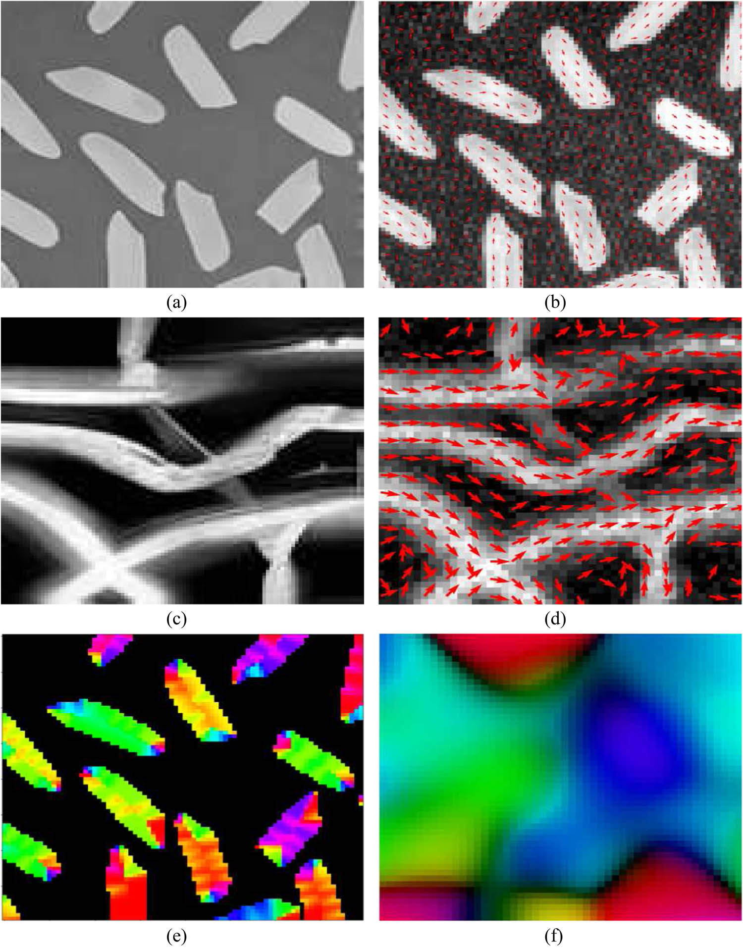
2D computational orientation vectors by ST analysis illustrating orientations and anisotropies. The ST is based on micro X-ray CT scans with low-resolution of fiber and grain microstructures. (a) Material grain, (b) anisotropic orientations, (c) material fiber, (d) anisotropic orientations, (e) degree of anisotropy in material grain, and (f) orientation and anisotropy in material fiber.

An important property of network structures is their orientations, based on two quantities. These quantities are the color of the image and the degree of anisotropy, superposed in a unique image to display orientation and anisotropy. The double eigenvalues represent this degree. In Figure 7(e)–(f), the oriented pattern is shown, underlying the anisotropic diffusion process. These distributions of angles, which are scalar values, specify mainly the direction as anisotropy characterization.

After reviewing the concept of a thorough analysis of the tensor estimation, we will present the attempts to extend the analysis definition to an additional dimension space in very simple gray scale of morphological images without CT scans. Quantitative wood images via 3D structure analysis require entirety much quantitative visualization [82,83]. Thus, the ST technique will be applied to various shape-simplifying images. First, the process is tested on these images, which are performed by their shape classes. Next, we will handle the wood images for our approach. The image features in straight lines and circular shapes are then investigated. These images indicate our created artificial dataset. It yields, of course, to defy purely the oriented description vector fields.

The above examples demonstrate our ability to preserve anisotropy features from patterns. The ST overall properties of the image features are well preserved, as shown in Figures 8 and 9. This is the most straightforward way to process those patterns’ estimated orientation, particularly the principal directions. Figure 8(c)–(d) shows the multi-dimensional orientation vectors on the fabric fibers expressed by straight line-type (see the 3D original image presented in Figure 8(a)). In 3D case, it can be stated that the typical distribution of principal directions follows well the sets of characteristic lines. In order to quantify these observations, the ST framework is generated bidimensionally and depicted in Figure 8(d). The purpose is to visualize potentially the coherent regions in vector fields. Here, two prevailing orientations exist. One of the material phase, which is presented continuously by lines, and one of the empty phase. For the energy field result, there are two color representations in which the high values are mapped to green to allow for a combined visualization of the vector fields, even in the empty zones. The energy information constitutes a coherent structure which is preserved to filter the directional preferences, as illustrated in Figure 8(b)–(d).

Figure 8

Result visualization of orientation maps using the ST technique applied at the continuous straight line fibers: (a) 3D input image, (b) 3D norm/energy, (c) 3D orientations, and (d) 2D orientations/energy.

Figure 9

3D estimated orientation related to the shape component of the cylindrical object tensor: (a) 3D input image, (b) 3D norm/energy, (c) 3D orientations, (d) 3D orientations (c) projected onto the plane Z = 0 , (e) 2D orientations/energy using σ = 0.5 and μ = 1 , and (f) 2D orientations/energy using σ = 0.2 and μ = 4 .

In the following, we construct a cylinder gravity model with the same center of the contained parallelepiped shape, which has equal length and width and a small height. Its diameter is equal to half-length. The 3D view of the synthetic model is shown in Figure 9(a). This model has the same voxel size as the input image presented in Figure 8(a). To demonstrate the real application effect, the ST approach is applied to the cylinder image. Then, the directional gradients of the input image are computed. The energy spectrum of the tensor field is shown in Figure 9(b). The projected orientations onto the plane from the synthetically image are compared with the 2D orientation obtained by the 2D ST, as shown in the three bottom diagrams of Figure 9(d). The ST is used for the anisotropic structure analysis to exhibit the energy and orientation patterns in the same map, as illustrated in Figure 9(f)–(e). The higher value of energy indicates highly oriented structures. Note that the combination vector field is calculated using the Gaussian kernel with parameters σ equal to 0.2 and μ equal to 4 (Figure 9(f)) being deemed sufficiently realistic for this study compared to the one defined with parameters σ equal to 0.5 and μ equal to 1 (Figure 9(e)). In other words, the local orientations are much more rotational in the case of high energy structure. We see that the estimation influences the Gaussian filter on the orientation maps in the higher-resolution data. Thus, the effect is relatively important. In both cases, the map is entirely different from the one projected map presented in Figure 9(d).

We have previously enhanced the structural anisotropy of images underlying some simplified geometrical objects. The anisotropy on a voxel level is quantified in terms of three independent scalar eigenvalues. Then, the third computed eigenvalue signifies the uncertainty concerning the dominant orientation of the structure field due to complex and noisy neighborhoods. Feature information, particularly orientation estimation of 3D images, is most important for computer vision and image processing. To estimate the LST, we will address responses for how to obtain the representation from computations on 3D image data. The proposed approach has been followed to realize this estimation and integrated in a visualization framework by the 3D VTK data [84]. For illustrative purposes, we will display the energy physics that has been applied to image processing. Estimating the local energy of wood species in different orientations is depicted in Figure 10. This energy is computed in terms of variation of the eigenvalues from the resulting tensor field. The variation is analyzed for two-phase wood material specimens. In other words, low-energy region is located in pores, while high-energy quantifies the tissue volumes. This is equivalent to saying that large eigenvalues of the ST at each pixel point mean high-frequency components of the image.

Figure 10

(a)–(b) The local energy of the structure corresponding to the detail view in 3D space for the poplar and spruce wood. A selection of 3D images have a resolution of 192 × 192 × 10 voxels and have different nodes to show the complexity of structure.

This work also aims at determining the anisotropic structure viewed as a set of direction vectors on the center points of the meshed microstructure. The process involved in the computation is the utilization of the mesh prepared from the tomographic micro-CT data. The CT scan image segmentation is based on using the Otsu thresholding method. Then, the material microstructure is triangulated to create the meshed surface using the open-source Nanomesh [85]. Recalling that Nanomesh is a Python workflow tool for creating 2D and 3D meshes from image data. The tool contains a pre-processing filter to segment the image data to generate a contour that accurately reports the phases of interest. This summarized that the meshing process consists of contour finding and triangulation. The local direction of the anisotropy defined on the voxel using the ST is correlated with the mesh center. Note that the image does not necessarily have to be segmented according to our framework to generate anisotropic diffusion of the ST. However, generating its mesh data via the thresholding concept is a required stage. There are various advantages to determine the preferred orientation on the featured geometrical elements. Particularly the stability and performance of mechanical and thermal frameworks strongly depend on anisotropic properties [86–90].

Figure 11 exhibits the local orientation presented by the anisotropy vector for the poplar and spruce wood specimens. The figure is divided into four diagrams that focus on the enlarged image in size to show the displayed vectors on the cell center highlighting the quality and morphology. The software tool used here for the visualization aspect is Paraview, in which the visualization was performed in VTK format. The proposed anisotropic morphology defined on the mesh can be explained as follows. The kernel-based approach defined on the mesh cell centers is associated with the nearest vector field computed from the local tensor at each pixel position. It means that the orientation estimation of a centered cell will be located close to the pixel position, which is given by distance information The applied mathematical morphology operation illustrates that there is a consistency from the anisotropic behavior depicted in Figure 3 compared to the presented below anisotropy.

Figure 11

2D visualization of the orientation vector field on the mesh for the wood species: (a) Poplar wood, (b) spruce wood, (c) the enlarged image presented in ( a ) , and (d) the enlarged image presented in ( b ) .

4 Comparison with other orientation analysis software

In contrast to some explored software tools, such as DiameterJ, OrientationJ, and FibrilTool, which are devoted to quantifying the fiber orientation analysis in 2D, our package is engaged on parameters especially required for biomaterials. The most regularly cited software tools for the investigation of fibrous materials are exhibited in Table 2, where the performance of software extensibility and integration with others software by users are analyzed. The proposed Python package, named Quanfima (quantitative analysis of fibrous materials) [91], offers both 2D and 3D analysis of data. It contains an assembly of useful routines designed for studying the morphological properties and composition under visualization of multi-dimensional data. The aim of using Quanfima is to provide a full analysis of wood materials, including the determination of fiber orientation, particle diameter, and porosity. The estimation of diameter quantifications is computed using a ray-casting method.

We run the anisotropic algorithm via Quanfima for the poplar and spruce wood specimens. The fiber network was visualized using the plugin Quanfima. The orientation angles are presented in degrees, varying from 0 to 180, and the diameter of each fiber is measured in pixels. The analysis of these fibrous materials is interpreted as follows. As shown in Figure 12, some solid tissues in increasing curves take the orange-green colors, and others with decreasing curves are attributed pink. The fabrics that follow or approach a rectilinear shape are assimilated to the red color. The fiber diameter given in the dataset impacts the computed throughput because a thicker fiber needs more iterations to catch a border. The diameter of the wood structures is investigated and presented by mapping geo-coordinates to a color scheme. Note that, concerning this diameter, our ST and Quanfima packages lead to the same result. As expected, large pore and vessel sizes, one of the key parameters in the main porosity properties, are identified inside a wood structure in pink and blue colors. The obtained results previously performed were expected because the morphological properties of the specimens react in the same way.

Figure 12

The morphological analysis from 2D fibrous data structures via quanfima package. These datasets are loaded from the previous gray scale image with the size of 352 × 352 . The visualization of the estimated orientation, analysis of the fiber orientation and diameters are shown in diagrams (a)–(b) (respectively (c)–(d)) for the poplar (respectively for the spruce) specimen.

Avizo is an object-oriented software system. It contains system components based on modules and data objects. For this purpose, there are two reasons that Avizo has not been presented in Table 2. The first is that it is commercial software supporting some file formats, such as Abaqus and ANSYS. The second consists of the difficulty of using the anisotropic module, particularly to view the orientation distribution on a 3D plot than 2D. The Avizo XWind provides tools and powerful visualization to display the vector tensor fields defined on 3D mesh-generated inputs. This aim of our developed package has been attempted in a simple way freely without processing main workflows on an image stack. There exists an implemented method in Avizo software to determine the orientation tensors, and the reader is referred to its documentation [92] for a detailed explanation. Using it allows visualizing the anisotropy of the wood by displaying the local directions. Avizo can visualize main orientation field given on 2D/3D Point Cloud sets or Line Sets. This offers the possibility to view the representation of points, rectangles, and line shapes as illustrated in Figure 13 corresponding to the orientations of the poplar material.

Figure 13

Visualization of anisotropy via Avizo for the poplar wood. The anisotropic behavior of local directions is displayed in point/rectangle (a) and line (b) forms.

5 Bidimentional orthotropic linear-elastic model with orientation

The purpose is to investigate the anisotropic behavior, depicting the elastic moduli that is considered important to understand and characterize the physical and mechanical properties [93–95]. Assuming that the investigated material is linear elastic with heterogeneous properties. In this elastic regime, according to Hooke’s law, it can be stated that for sufficiently low stresses, the stress σ is proportional to the magnitude of the strain ε . Thus, in the Voigt notation, this can be expressed via the local stiffness matrix C , i.e., σ = C ε ,

C is the symmetric 3 × 3 matrix characterized by four independent coefficients to model the anisotropic wood materials in 2D space. The elastic coefficients matrix C i j are expressed in terms of the elastic coefficients, which are Young’s moduli E 1 and E 2 , Poisson’s ratios ν 12 and ν 21 , and one shear moduli G 12 . The mechanical and elastic properties are described within these coefficients, which are given as follows:

Also, as an alternative to equation (22),

where C i j k l are the fourth-rank elastic stiffness tensor, and σ i j and ε k l denote the homogeneous second-rank tensors. This means that the stiffness tensor is often written using the two-index convention C m n , expressed in equation (22), where m and n are related to the four indices i j k l expressed in equation (24) with respect to specific ordering. Conversely, the inverse of Hooke’s law takes the following form ε = S σ , where S is the compliance matrix, defined by inverting the stiffness matrix C , i.e., S = C − 1 . The symmetry of the compliance matrix implies the relationship between the engineering constant

The purpose is to investigate the conceived model to general anisotropic microstructural materials within a given rotational angle [96–98]. Consider a generic coordinate system x y rotated by the angle θ with respect to the initial system. Then, σ ˆ denotes the stress tensor in the new orientation coordinate system expressed in terms of the stress tensor σ conforming to the elementary rotational matrix R

Similarly, the strain tensor ε ˆ in the new reference basis is expressed as

Then, equation (22) can be rewritten as Hook’s law in the new reference basis

Equations (26)–(27) and (22)–(28) can be coupled between them, yielding the compact expression [30,99,100],

Summarizing based on the aforementioned work, the results of anisotropic elasticity gained for the 2D Cauchy continuum within the new tensor C ˆ are transferred from the tensor terms C , C ˆ = G : C ,

where G is the orientation tensor expressed in terms of the rotation matrix elements.

We refer the reader to the previous excellent works [101,102] exploring the mechanical properties within the FE modeling based on the wood samples along the three orthotropic directions. This study is investigated in the 3D organization where the material directions, namely radial (R), tangential (T), and longitudinal (L). A reduction of 1D in space refers to the 2D case without the longitudinal direction. In order to examine the 2D mechanical behavior of the wood specimens, the FE simulations are conducted with the spruce wood microstructure. The aim here is to show the ability of the framework to generate the different material properties. For that, the mechanical properties used in the model are assumed to be constant and independent of the porosity. This assumption is explained by simplifying the modeling work. The purpose is to determine the better physical engineering coefficients used in the literature for which the framework is convergent and affects the numerical results. Neagu and Gamstedt [103] study principally the knowledge of the anatomical features structured from the wood fiber while dispensing the hygroelastic properties from these samples. The radial and longitudinal Young’s moduli E 1 and E 2 of the wood specimen is equal to 6.08 GPa, E 1 = E 2 = 6.08 GPa. Poisson’s ratio ν 12 and the shear moduli G 12 for transverse strain in the tangential direction (T) when stress applies in the radial direction (R), are respectively, 0.42 and 2.14 GPa. Formally, ν 12 = 0.42 GPa, G 12 = 2.14 GPa.

Figure 14 reports the FE numerical results of testing the wood microstructure with highlighting 2D mechanical analysis. The figure is shared into six diagrams, depicting each component microstructure’s mechanical distributions. This investigated microstructure is the spruce wood specimen having the dimension of 192 × 192 pixels, and treated with ImageJ-Python software. The FE approach takes as input the meshing geometry, with the channel loads in terms of the displacement boundary conditions. Note that the presented FE framework is designed for the orthotropic elastic problems, implemented without the previously rotated formalism. First, the material microstructure was meshed in 2D, 3D triangular elements using an automatic mesh generator (nanomesh) [85]. The model contained approximately 1,000 elements and approximately 1,000-half nodes. The boundary conditions should be enforced. The vertical displacements are applied to the top boundary layer of the microstructure. However, the inferior and four rest lateral sides are considered blocked. This means that there is a null displacement on these sides, as illustrated in Figure 14(f) in which the deformed shapes and displacement maps are obtained with the FE analyses.

Figure 14

The mechanical test under the tensile loading demonstrates the validation of the orthotropic linear-elastic model in 2D space for the spruce wood microstructure image with the size of 192 × 192 . The specimen is characterized by the mechanical properties within Young’s moduli, E 1 = E 2 = 6.08 GPa, the Poisson’s ratio ν 12 , and the shear moduli G 12 , i.e., ν 12 = 0.42 GPa, G 12 = 2.14 GPa. (a) Displacement field u 22 , (b) component of strain ε 22 , (c) component of stress σ 22 , (d) displacement field u 11 , (e) component of stress σ 11 , and (f) original/deformed shape.

The FE modeling is confirmed against some uniaxial mechanical testing responding to the tensile loadings. As said before, the Dirichlet boundary conditions are defined by enforcing a vertical displacement − 4 × 1 0 − 6 on the top nodes following the tangential direction T corresponding to the y -axis. The radial strain tensor ε 22 is calculated according to the strain–displacement relation, i.e., ε = B u , where B is the strain–displacement matrix (Figure 14(b)). According to the stress–strain relationship given by equality (22), the component of stress σ 22 is calculated and its variation is illustrated in Figure 14(c). Figure 14(d) and (e) depict the radial displacement and stress fields. The modeling results show that it is consistent with respect to the expected computations, particularly the Poisson effect. At first sight, the Poisson effect is illustrated in the top diagrams. Particularly, as shown in Figure 14(a) when the tangential displacement u 22 varies steadily from the lower value − 4 × 1 0 − 6 to the higher value 2.6 × 1 0 − 9 .

6 Summary and future work

Throughout the article, we have used the ST model on wood images to construct quantitative fiber orientation maps in 2D and 3D spaces. The ST is typically used to extract features on digital images. This consists of taking a pixel’s neighboring gradients into account to provide the anisotropy and directionality. In the industry sector, this serves to predict these mechanical properties in the global axis system, minimizing the production costs in time. Investigation of wood anisotropy aims to tackle the major commercial obstacles of new biomaterials produced from wood by reducing their costs. First, the ST-based fiber orientation mapping is presented on the plane. Since the analogy of ST with the tensor matrices in 3D remains the same, its extension into the 3D space remains the same. Efforts in the computational analysis have been made to implement the software tools via imaging techniques using the performant visual interfaces. The computational orientation maps demonstrate a good agreement of directional information extracted from the imaging system. We will demonstrate that the vector corresponding to orientation maps is not sensitive to image intensity and is independent of the preprocessing filter. The reason is the compatibility between the 2D/3D computational orientation vectors and the morphology of the original microstructure. This comparison correlates well with the computed orientations and morphology. This information has been provided and is available with direct viewing at tensors from a visualization point of view. Moreover, the results obtained from the 3D ST analysis remains ambiguous of directional alignments. Particularly, the lack of a dominant direction to be observed visually. To clarify this ambiguity, the orientation map on the horizontal and vertical planes is displayed.

References

[1] Kratz, A., C. Auer, M. Stommel, and I. Hotz. Visualization and analysis of second-order tensors: Moving beyond the symmetric positive-definite case. In: Computer Graphics Forum, vol. 32, 2013, pp. 49–74. Wiley Online Library. 10.1111/j.1467-8659.2012.03231.xSearch in Google Scholar
[2] Maurizi, M., C. Gao, and F. Berto Predicting stress, strain and deformation fields in materials and structures with graph neural networks. Scientific Reports, Vol. 12, No. 1, 2022, 21834. 10.1038/s41598-022-26424-3Search in Google Scholar PubMed PubMed Central
[3] Chakkour, T. Application of two-dimensional finite volume method to protoplanetary disks. International Journal of Mechanics, Vol. 15, 2021, pp. 233–245. 10.46300/9104.2021.15.27Search in Google Scholar
[4] Chakkour, T. and F. Benkhaldoun. Slurry pipeline for fluid transients in pressurized conduits. International Journal of Mechanics, Vol. 14, 2020, pp. 1–11. 10.46300/9104.2020.14.1Search in Google Scholar
[5] Chakkour, T. Numerical simulation of pipes with an abrupt contraction using openFOAM. Fluid Mechanics at Interfaces 2: Case Studies and Instabilities, Wiley, 2022, pp. 45–75. 10.1002/9781119903000.ch3Search in Google Scholar
[6] Karimi, D. and A. Gholipour. Diffusion tensor estimation with transformer neural networks. Artificial intelligence in medicine, Vol. 130, 2022, id. 102330. 10.1016/j.artmed.2022.102330Search in Google Scholar PubMed PubMed Central
[7] Chen, Y., Y. Wang, Z. Song, Y. Fan, T. Gao, and X. Tang. Abnormal white matter changes in Alzheimer’s disease based on diffusion tensor imaging: A systematic review. Ageing Research Reviews, Vol. 87, 2023, pp. 101911. 10.1016/j.arr.2023.101911Search in Google Scholar PubMed
[8] Magdoom, K. N., A. V. Avram, J. E. Sarlls, G. Dario, and P. J. Basser. A novel framework for in-vivo diffusion tensor distribution MRI of the human brain. NeuroImage, Vol. 271, 2023, id. 120003. 10.1016/j.neuroimage.2023.120003Search in Google Scholar PubMed PubMed Central
[9] Santos, L. A., B. Sullivan, O. Kvist, S. Jambawalikar, S. Mostoufi-Moab, J. M. Raya, et al. Diffusion tensor imaging of the physis: the abc’s. Pediatric radiology, Vol. 53, No. 12, 2023, pp. 2355–2368. 10.1007/s00247-023-05753-zSearch in Google Scholar PubMed PubMed Central
[10] Kazmierczak, N. P., M. Van Winkle, C. Ophus, K. C. Bustillo, S. Carr, H. G. Brown, et al. Strain fields in twisted bilayer graphene. Nature materials, Vol. 20, No. 7, 2021, pp. 956–963. 10.1038/s41563-021-00973-wSearch in Google Scholar PubMed
[11] Guerrero, J., T. A. Gallagher, A. L. Alexander, and A. S. Field. Diffusion tensor magnetic resonance imaging-physical principles. In: Functional Neuroradiology: Principles and Clinical Applications, 2023, pp. 903–932. Springer. 10.1007/978-3-031-10909-6_39Search in Google Scholar
[12] Domingues, T. S., R. R. Coifman, and A. Haji-Akbari. Robust estimation of position-dependent anisotropic diffusivity tensors from stochastic trajectories. The Journal of Physical Chemistry B, Vol. 127, No. 23, 2023, pp. 5273–5287. 10.1021/acs.jpcb.3c00670Search in Google Scholar PubMed
[13] Yurovsky, V. and I. Kudryashov. Anisotropic cosmic ray diffusion tensor in a numerical experiment. Bulletin of the Russian Academy of Sciences: Physics, Vol. 87, No. 7, 2023, pp. 1032–1034. 10.3103/S1062873823702337Search in Google Scholar
[14] Tian, Q., B. Bilgic, Q. Fan, C. Liao, C. Ngamsombat, Y. Hu. Deepdti: High-fidelity six-direction diffusion tensor imaging using deep learning. NeuroImage, Vol. 219, 2020, id. 117017. 10.1016/j.neuroimage.2020.117017Search in Google Scholar PubMed PubMed Central
[15] Karamov, R., L. M. Martulli, M. Kerschbaum, I. Sergeichev, Y. Swolfs, and S. V. Lomov. Micro-ct based structure tensor analysis of fibre orientation in random fibre composites versus high-fidelity fibre identification methods. Composite Structures, Vol. 235, 2020, id. 111818. 10.1016/j.compstruct.2019.111818Search in Google Scholar
[16] Tatekawa, H., S. Matsushita, D. Ueda, H. Takita, D. Horiuchi, N. Atsukawa Improved reproducibility of diffusion tensor image analysis along the perivascular space (dti-alps) index: an analysis of reorientation technique of the oasis-3 dataset. Japanese Journal of Radiology, Vol. 41, No. 4, 2023, pp. 393–400. 10.1007/s11604-022-01370-2Search in Google Scholar PubMed PubMed Central
[17] Deng, Y.-J., H.-C. Li, S.-Q. Tan, J. Hou, Q. Du, and A. Plaza. t-linear tensor subspace learning for robust feature extraction of hyperspectral images. IEEE Transactions on Geoscience and Remote Sensing, Vol. 61, 2023, pp. 1–15. 10.1109/TGRS.2023.3233945Search in Google Scholar
[18] Westin, C. F., S. E. Maier, B. Khidhir, P. Everett, F. A. Jolesz, and R. Kikinis Image processing for diffusion tensor magnetic resonance imaging. In Medical Image Computing and Computer-Assisted Intervention-MICCAI-99: Second International Conference, Cambridge, UK, September 19–22, 1999. Proceedings 2, pp. 441–452, Springer, 1999. 10.1007/10704282_48Search in Google Scholar
[19] Panagakis, Y., J. Kossaifi, G. G. Chrysos, J. Oldfield, M. A. Nicolaou, A. Anandkumar, et al. Tensor methods in computer vision and deep learning. Proceedings of the IEEE, Vol. 109, No. 5, 2021, pp. 863–890. 10.1109/JPROC.2021.3074329Search in Google Scholar
[20] Jung, H., Y. Kim, H. Jang, N. Ha, and K. Sohn. Unsupervised deep image fusion with structure tensor representations. IEEE Transactions on Image Processing, Vol. 29, 2020, id. 3845–3858. 10.1109/TIP.2020.2966075Search in Google Scholar PubMed
[21] Auenhammer, R. M., A. Prajapati, K. Kalasho, L. P. Mikkelsen, P. J. Withers, L. E. Asp, and R. Gutkin. Fibre orientation distribution function mapping for short fibre polymer composite components from low resolution/large volume x-ray computed tomography. Composites Part B: Engineering, 2024, id. 111313. 10.1016/j.compositesb.2024.111313Search in Google Scholar
[22] Ali, M. A., T. Khan, K. A. Khan, and R. Umer. Micro computed tomography based stochastic design and flow analysis of dry fiber preforms manufactured by automated fiber placement. Journal of Composite Materials, Vol. 57, No. 12, 2023, pp. 2075–2090. 10.1177/00219983231168791Search in Google Scholar
[23] Maurer, J., D. Salaberger, M. Jerabek, B. Fröhler, J. Kastner, and Z. Major. Fibre and failure characterization in long glass fibre reinforced polypropylene by x-ray computed tomography. Polymer Testing, Vol. 130, 2024, id. 108313. 10.1016/j.polymertesting.2023.108313Search in Google Scholar
[24] Trussell, N., M. S. Hårr, G. Kjeka, I. Asadi, P. E. Endrerud, and S. Jacobsen. Anisotropy and macro porosity in wet sprayed concrete: Laminations, fibre orientation and macro pore properties measured by image analysis, pf test, water penetration and ct scanning. Construction and Building Materials, Vol. 389, 2023, id. 131715. 10.1016/j.conbuildmat.2023.131715Search in Google Scholar
[25] Zanuttini, R. and F. Negro. Wood-based composites: Innovation towards a sustainable future. Forests, Vol. 12, 2021, id. 1717. 10.3390/f12121717Search in Google Scholar
[26] Guo, F., J. Wang, W. Liu, J. Hu, Y. Chen, X. Zhang, R. Yang, and Y. Yu. Role of microfibril angle in molecular deformation of cellulose fibrils in Pinus massoniana compression wood and opposite wood studied by in-situ waxs. Carbohydrate Polymers, Vol. 334, 2024, id. 122024. 10.1016/j.carbpol.2024.122024Search in Google Scholar PubMed
[27] Purba, C. Y. C., J. Dlouha, J. Ruelle, and M. Fournier. Mechanical properties of secondary quality beech (fagus sylvatica l.) and oak (quercus petraea (matt.) liebl.) obtained from thinning, and their relationship to structural parameters. Annals of Forest Science, Vol. 78, 2021, pp. 1–11. 10.1007/s13595-021-01103-xSearch in Google Scholar
[28] Mirkhalaf, S., E. Eggels, T. Van Beurden, F. Larsson, and M. Fagerström. A finite element based orientation averaging method for predicting elastic properties of short fiber reinforced composites. Composites Part B: Engineering, Vol. 202, 2020, id. 108388. 10.1016/j.compositesb.2020.108388Search in Google Scholar
[29] Reinold, J., V. Gudžulić, and G. Meschke. Computational modeling of fiber orientation during 3d-concrete-printing. Computational Mechanics, Vol. 71, No. 6, 2023, pp. 1205–1225. 10.1007/s00466-023-02304-zSearch in Google Scholar
[30] Zhang, P., R. Abedi, and S. Soghrati. A finite element homogenization-based approach to analyze anisotropic mechanical properties of chopped fiber composites using realistic microstructural models. Finite Elements in Analysis and Design, Vol. 235, 2024, id. 104140. 10.1016/j.finel.2024.104140Search in Google Scholar
[31] Annasabi, Z. and F. Erchiqui. 3d hybrid finite elements for anisotropic heat conduction in a multi-material with multiple orientations of the thermal conductivity tensors. International Journal of Heat and Mass Transfer, Vol. 158, 2020, id. 119795. 10.1016/j.ijheatmasstransfer.2020.119795Search in Google Scholar
[32] Ferguson, O. V. and L. P. Mikkelsen. Three-dimensional finite element modeling of anisotropic materials using x-ray computed micro-tomography data. Software Impacts, Vol. 17, 2023, id. 100523. 10.1016/j.simpa.2023.100523Search in Google Scholar
[33] Tang, H., H. Chen, Q. Sun, Z. Chen, and W. Yan. Experimental and computational analysis of structure-property relationship in carbon fiber reinforced polymer composites fabricated by selective laser sintering. Composites Part B: Engineering, Vol. 204, 2021, id. 108499. 10.1016/j.compositesb.2020.108499Search in Google Scholar
[34] Kugler, S. K., A. Kech, C. Cruz, and T. Osswald. Fiber orientation predictions-a review of existing models. Journal of Composites Science, Vol. 4, No. 2, 2020, id. 69. 10.3390/jcs4020069Search in Google Scholar
[35] Wang, Z., C. Luo, Z. Xie, and Z. Fang. Three-dimensional polymer composite flow simulation and associated fiber orientation prediction for large area extrusion deposition additive manufacturing. Polymer Composites, Vol. 44, No. 10, 2023, pp. 6720–6735. 10.1002/pc.27591Search in Google Scholar
[36] Ennis, D. B. and G. Kindlmann. Orthogonal tensor invariants and the analysis of diffusion tensor magnetic resonance images. Magnetic Resonance in Medicine: An Official Journal of the International Society for Magnetic Resonance in Medicine, Vol. 55, No. 1, 2006, pp. 136–146. 10.1002/mrm.20741Search in Google Scholar PubMed
[37] Tornifoglio, B., A. Stone, R. Johnston, S. Shahid, C. Kerskens, and C. Lally Diffusion tensor imaging and arterial tissue: establishing the influence of arterial tissue microstructure on fractional anisotropy, mean diffusivity and tractography. Scientific Reports, Vol. 10, No. 1, 2020, id. 20718. 10.1038/s41598-020-77675-xSearch in Google Scholar PubMed PubMed Central
[38] Jähne, B. Digital Image Processing. Springer Science & Business Media, Springer Berlin, Heidelberg, 2005. Search in Google Scholar
[39] Förstner, W. and E. Gülch. A fast operator for detection and precise location of distinct points, corners and centres of circular features. In: Proc. ISPRS Intercommission Conference on Fast Processing of Photogrammetric Data, vol. 6, 1987, pp 281–305. Interlaken. Search in Google Scholar
[40] Jähne, B. Spatio-temporal Image Processing: Theory and Scientific Applications. Springer, Springer Berlin, Heidelberg, 1993.10.1007/3-540-57418-2Search in Google Scholar
[41] Bigun, J., T. Bigun, and K. Nilsson. Recognition by symmetry derivatives and the generalized structure tensor. IEEE Transactions on Pattern Analysis and Machine Intelligence, Vol. 26, No. 12, 2004, pp. 1590–1605. 10.1109/TPAMI.2004.126Search in Google Scholar PubMed
[42] Koyan, P. and J. Tronicke. 3d ground-penetrating radar data analysis and interpretation using attributes based on the gradient structure tensor. Geophysics, Vol. 89, No. 4, 2024, pp. 1–39. 10.1190/geo2023-0670.1Search in Google Scholar
[43] Dinh, P.-H., V.-H. Vu, N. L. Giang, et al. A new approach to medical image fusion based on the improved extended difference-of-gaussians combined with the coati optimization algorithm. Biomedical Signal Processing and Control, Vol. 93, 2024, id. 106175. 10.1016/j.bspc.2024.106175Search in Google Scholar
[44] Beghini, M., T. Grossi, M. B. Prime, and C. Santus. Ill-posedness and the bias-variance tradeoff in residual stress measurement inverse solutions. Experimental Mechanics, Vol. 63, No. 3, 2023, pp. 495–516. 10.1007/s11340-022-00928-5Search in Google Scholar
[45] Bénard, P.-J., Y. Traonmilin, J.-F. Aujol, and E. Soubies. Estimation of off-the grid sparse spikes with over-parametrized projected gradient descent: theory and application. Inverse Problems, Vol. 40, No. 5, 2024, id. 055010. 10.1088/1361-6420/ad33e4Search in Google Scholar
[46] Hassan, T., S. Akcay, B. Hassan, M. Bennamoun, S. Khan, J. Dias, and N. Werghi. Cascaded structure tensor for robust baggage threat detection. Neural Computing and Applications, Vol. 35, No. 15, 2023, pp. 11269–11285. 10.1007/s00521-023-08296-4Search in Google Scholar
[47] Gerber, T. A., D. A. Lilien, N. M. Rathmann, S. Franke, T. J. Young, F. Valero-Delgado, M. R. Ershadi, R. Drews, O. Zeising, A. Humbert, et al. Crystal orientation fabric anisotropy causes directional hardening of the Northeast Greenland ice stream. Nature Communications, Vol. 14, No. 1, 2023, id. 2653. 10.1038/s41467-023-38139-8Search in Google Scholar PubMed PubMed Central
[48] Pannier, Y., P. Coupé, T. Garrigues, M. Gueguen, and P. Carré. Automatic segmentation and fibre orientation estimation from low resolution x-ray computed tomography images of 3d woven composites. Composite Structures, Vol. 318, 2023, id. 117087. 10.1016/j.compstruct.2023.117087Search in Google Scholar
[49] De Pascalis, F., F. Lionetto, A. Maffezzoli, and M. Nacucchi. A general approach to calculate the stiffness tensor of short-fiber composites using the fabric tensor determined by x-ray computed tomography. Polymer Composites, Vol. 44, No. 2, 2023, pp. 917–931. 10.1002/pc.27143Search in Google Scholar
[50] Anderson, C., C. Ntala, A. Ozel, R. L. Reuben, and Y. Chen. Computational homogenization of histological microstructures in human prostate tissue: Heterogeneity, anisotropy and tension-compression asymmetry. International Journal for Numerical Methods in Biomedical Engineering, Vol. 39, No. 11, 2023, e3758. 10.1002/cnm.3758Search in Google Scholar PubMed PubMed Central
[51] Nejim, Z., L. Navarro, C. Morin, and P. Badel. Quantitative analysis of second harmonic generated images of collagen fibers: a review. Research on Biomedical Engineering, Vol. 39, No. 1, 2023, pp. 273–295. 10.1007/s42600-022-00250-ySearch in Google Scholar
[52] Al Ayoubi, N. A., H. Digonnet, L. Silva, C. Binetruy, T. Renault, and S. Comas-Cardona. Simulation of the fiber orientation through a finite element approach to solve the fokker-planck equation. Journal of Non-Newtonian Fluid Mechanics, Vol. 331, 2024, id. 105284. 10.1016/j.jnnfm.2024.105284Search in Google Scholar
[53] Beigzadeh, S. and J. E. Shield. Utilizing local orientation image analysis for microstructure quantification in additive manufacturing. Materials Characterization, Vol. 210, 2024, id. 113761. 10.1016/j.matchar.2024.113761Search in Google Scholar
[54] Chakkour, T. Some inverse problem remarks of a continuous-in-time financial model in l 1 ([ti, θ max]). Mathematical Modeling and Computing, Vol. 10, No. 3, 2023, pp. 864–874.10.23939/mmc2023.03.864Search in Google Scholar
[55] Chakkour, T. Inverse problem stability of a continuous-in-time financial model. Acta Mathematica Scientia. Vol. 39, 2019, pp. 1423–1439. 10.1007/s10473-019-0519-5Search in Google Scholar
[56] Yadav, R. P., I. Rago, F. Pandolfi, C. Mariani, A. Ruocco, S. Tayyab. Evaluation of vertical alignment in carbon nanotubes: A quantitative approach. Nuclear Instruments and Methods in Physics Research Section A: Accelerators, Spectrometers, Detectors and Associated Equipment, Vol. 1060, 2024, id. 169081. 10.1016/j.nima.2024.169081Search in Google Scholar
[57] Rahman, C. M. A. and H. Nyeem. Tensor-enhanced shock energy-driven active contours: A novel approach for knowledge-based image segmentation. Journal of Visual Communication and Image Representation, Vol. 103, 2024, id. 104218. 10.1016/j.jvcir.2024.104218Search in Google Scholar
[58] Métivier, L., R. Brossier, A. Hoffmann, J.-M. Mirebeau, G. Provenzano, A. Tarayoun, and P. Yong. Coherence-enhancing anisotropic diffusion filter for 3d high-resolution reconstruction of p-wave velocity and density using full-waveform inversion: Application to a north sea ocean bottom cable data set. Geophysics, Vol. 89, No. 1, 2024, pp. R33–R58. 10.1190/geo2022-0648.1Search in Google Scholar
[59] Bauer, J. K. and T. Böhlke. Fiber orientation distributions based on planar fiber orientation tensors of fourth order. Mathematics and Mechanics of Solids, Vol. 28, No. 3, 2023, pp. 773–794. 10.1177/10812865221093958Search in Google Scholar
[60] Malikan, M., S. Dastjerdi, V. A. Eremeyev, and H. M. Sedighi. On a 3d material modelling of smart nanocomposite structures. International Journal of Engineering Science, Vol. 193, 2023, id. 103966. 10.1016/j.ijengsci.2023.103966Search in Google Scholar
[61] Liu, G., K. Huang, Y. Zhong, Z. Li, H. Yu, L. Guo, and S. Li. Investigation on the off-axis tensile failure behaviors of 3d woven composites through a coupled numerical-experimental approach. Thin-Walled Structures, Vol. 192, 2023a, id. 111176. 10.1016/j.tws.2023.111176Search in Google Scholar
[62] Yang, J., Z. Guo, B. Wu, and S. Du. A nonlinear anisotropic diffusion model with non-standard growth for image segmentation. Applied Mathematics Letters, Vol. 141, 2023, id. 108627. 10.1016/j.aml.2023.108627Search in Google Scholar
[63] Magat, J., V. Ozenne, N. Cedilnik, J. Naulin, K. Haliot, M. Sermesant, et al. 3d MRI of explanted sheep hearts with submillimeter isotropic spatial resolution: comparison between diffusion tensor and structure tensor imaging. Magnetic Resonance Materials in Physics, Biology and Medicine. 2021. pp. 1–15. 10.1007/s10334-021-00913-4Search in Google Scholar PubMed PubMed Central
[64] Mahmood, M. T. and I. H. Lee. Shape from focus based on 3d structure tensor using optical microscopy. Microscopy Research and Technique, Vol. 83, No. 1, 2020, pp. 48–55. 10.1002/jemt.23386Search in Google Scholar PubMed
[65] Iske, A. and T. Randen. Methods and Modelling in Hydrocarbon Exploration and Production. Springer, Springer Berlin, Heidelberg, 2005. 10.1007/b137702Search in Google Scholar
[66] O’Shea, D., M. Attard, and D. Kellermann. Anisotropic hyperelasticity using a fourth-order structural tensor approach. International Journal of Solids and Structures, Vol. 198, 2020, id. 149–169. 10.1016/j.ijsolstr.2020.03.021Search in Google Scholar
[67] Chakkour, T. Parallel computation to bidimensional heat equation using MPI/CUDA and FFTW package. Frontiers in Computer Science, Vol. 5, 2024c, pp. 1305800–1305813. 10.3389/fcomp.2023.1305800Search in Google Scholar
[68] Shkarin, R., S. Shkarina, V. Weinhardt, R. A. Surmenev, M. A. Surmeneva, A. Shkarin. GPU-accelerated ray-casting for 3d fiber orientation analysis. Plos One, Vol. 15, No. 7, 2020, e0236420. 10.1371/journal.pone.0236420Search in Google Scholar PubMed PubMed Central
[69] Chakkour, T. High-quality implementation for a continuous-in-time financial API in c#. Frontiers in Computer Science, Vol. 6, 2024b. pp. 1371052–1371081. 10.3389/fcomp.2024.1371052Search in Google Scholar
[70] Wielhorski, Y., A. Mendoza, M. Rubino, and S. Roux. Numerical modeling of 3d woven composite reinforcements: A review. Composites Part A: Applied Science and Manufacturing, Vol. 154, 2022, id. 106729. 10.1016/j.compositesa.2021.106729Search in Google Scholar
[71] Yin, X., Q. Li, X. Xu, B. Chen, K. Guo, and S. Xu. Investigation of continuous surface cap model (CSCM) for numerical simulation of strain-hardening fibre-reinforced cementitious composites against low-velocity impacts. Composite Structures, Vol. 304, 2023, id. 116424. 10.1016/j.compstruct.2022.116424Search in Google Scholar
[72] Rondina, F., M. P. Falaschetti, N. Zavatta, and L. Donati. Numerical simulation of the compression crushing energy of carbon fiber-epoxy woven composite structures. Composite Structures, Vol. 303, 2023, id. 116300. 10.1016/j.compstruct.2022.116300Search in Google Scholar
[73] Otsu, N. A threshold selection method from gray-level histograms. Automatica, Vol. 11, No. 285–296, 1975, pp. 23–27. Search in Google Scholar
[74] Vondřejc, J., D. Liu, M. Ladeckỳ, and H. G. Matthies. FFT-based homogenisation accelerated by low-rank tensor approximations. Computer Methods in Applied Mechanics and Engineering, Vol. 364, 2020, id. 112890. 10.1016/j.cma.2020.112890Search in Google Scholar
[75] Liu, Y., J. Liu, Z. Long, and C. Zhu. Tensor Computation for Data Analysis. 2022, Springer, Springer Cham. 10.1007/978-3-030-74386-4Search in Google Scholar
[76] Liu, K., W. Xu, H. Wu, and A. A. Yahya. Weighted hybrid order total variation model using structure tensor for image denoising. Multimedia Tools and Applications, Vol. 82, No. 1, 2023b, pp. 927–943. 10.1007/s11042-022-12393-2Search in Google Scholar
[77] Kidangan, R. T., S. Unnikrishnakurup, C. Krishnamurthy, and K. Balasubramaniam. Uncovering the hidden structure: A study on the feasibility of induction thermography for fiber orientation analysis in CFRP composites using 2d-FFT. Composites Part B: Engineering, Vol. 269, 2024, id. 111107. 10.1016/j.compositesb.2023.111107Search in Google Scholar
[78] Sorelli, M., I. Costantini, L. Bocchi, M. Axer, F. S. Pavone, and G. Mazzamuto Fiber enhancement and 3d orientation analysis in label-free two-photon fluorescence microscopy. Scientific Reports, Vol. 13, No. 1, 2023, id. 4160. 10.1038/s41598-023-30953-wSearch in Google Scholar PubMed PubMed Central
[79] Dias, P. A., R. J. Rodrigues, and M. S. Reis. Fast characterization of in-plane fiber orientation at the surface of paper sheets through image analysis. Chemometrics and Intelligent Laboratory Systems, Vol. 234, 2023, id. 104761. 10.1016/j.chemolab.2023.104761Search in Google Scholar
[80] Liu, W. and E. Ralston. A new directionality tool for assessing microtubule pattern alterations. Cytoskeleton, Vol. 71, No. 4, 2014, pp. 230–240. 10.1002/cm.21166Search in Google Scholar PubMed PubMed Central
[81] Czarnecka, K., M. Wojasiński, T. Ciach, and P. Sajkiewicz. Solution blow spinning of polycaprolactone-rheological determination of spinnability and the effect of processing conditions on fiber diameter and alignment. Materials, Vol. 14, No. 6, 2021, 1463. 10.3390/ma14061463Search in Google Scholar PubMed PubMed Central
[82] Trtik, P., J. Dual, D. Keunecke, D. Mannes, P. Niemz, P. Stähli. 3d imaging of microstructure of spruce wood. Journal of structural biology, Vol. 159, No. 1, 2007, pp. 46–55. 10.1016/j.jsb.2007.02.003Search in Google Scholar PubMed
[83] Shi, J., X. Liu, C. Xia, W. Leng, and W. Li. Visualization of wood cell structure during cellulose purification via high resolution x-ray ct and spectroscopy. Industrial Crops and Products, Vol. 189, 2022, id. 115869. 10.1016/j.indcrop.2022.115869Search in Google Scholar
[84] Kitware Inc., the visualization toolkit. 2004. https://vtk.org/.Search in Google Scholar
[85] Smeets, S., N. Renaud, and L. J. C. van Willenswaard. Nanomesh: A python workflow tool for generating meshes from image data. Journal of Open Source Software, Vol. 7, No. 78, 2022, id. 4654. 10.21105/joss.04654Search in Google Scholar
[86] Guan, J., G. Ying, L. Liu, and L. Guo. A thermal-mechanical coupled bond-based peridynamic model for fracture of anisotropic materials. International Journal of Heat and Mass Transfer, Vol. 231, 2024, id. 125848. 10.1016/j.ijheatmasstransfer.2024.125848Search in Google Scholar
[87] Zhang, J., T. Luo, D. Zhang, S. Yin, H. He, and J. Peng. Multi-objective topology optimization of thermal-mechanical coupling anisotropic structures using the isogeometric analysis approach. Applied Mathematical Modelling, Vol. 117, 2023, pp. 267–285. 10.1016/j.apm.2022.12.014Search in Google Scholar
[88] Ai, Z. Y. and W. Y. Feng. The mechanical response of energy pile groups in layered cross-anisotropic soils under vertical loadings. Energy, Vol. 292, 2024, id. 130531. 10.1016/j.energy.2024.130531Search in Google Scholar
[89] Zhou, T., Y. Zhao, and Z. Rao. Fundamental and estimation of thermal contact resistance between polymer matrix composites: A review. International Journal of Heat and Mass Transfer, Vol. 189, 2022, id. 122701. 10.1016/j.ijheatmasstransfer.2022.122701Search in Google Scholar
[90] Park, I., J. Moon, S. Bae, J. E. Oh, and S. Yoon. Application of micro-ct to mori-tanaka method for non-randomly oriented pores in air-entrained cement pastes. Construction and Building Materials, Vol. 255, 2020, id. 119342. 10.1016/j.conbuildmat.2020.119342Search in Google Scholar
[91] Shkarin, R., A. Shkarin, S. Shkarina, A. Cecilia, R. A. Surmenev, M. A. Surmeneva. Quanfima: An open source python package for automated fiber analysis of biomaterials. PLoS One, Vol. 14, No. 4, 2019, e0215137. 10.1371/journal.pone.0215137Search in Google Scholar PubMed PubMed Central
[92] Thermoscientic avizo software 9 user’s guide. Technical report. Accessed January 2024, 2024. Search in Google Scholar
[93] Nie, Z., H. Jiang, and L. B. Kara. Stress field prediction in cantilevered structures using convolutional neural networks. Journal of Computing and Information Science in Engineering, Vol. 20, No. 1, 2020, id. 011002. 10.1115/1.4044097Search in Google Scholar
[94] Florisson, S., M. Hartwig, M. Wohlert, and E. K. Gamstedt. Microscopic computed tomography aided finite element modelling as a methodology to estimate hygroexpansion coefficients of wood: a case study on opposite and compression wood in softwood branches. Holzforschung, Vol. 77, No. 9, 2023, pp. 700–712. 10.1515/hf-2023-0014Search in Google Scholar
[95] Yang, D., H. Li, Y. Wu, C. Hong, R. Lorenzo, and C. Yuan. Experimental and finite element modelling analysis on the embedment performance and failure mechanisms of flattened-bamboo composite with the effect of fiber orientation angle. Construction and Building Materials, Vol. 445, 2024, id. 137929. 10.1016/j.conbuildmat.2024.137929Search in Google Scholar
[96] Varandas, L. F., G. Catalanotti, A. R. Melro, R. Tavares, and B. G. Falzon. Micromechanical modelling of the longitudinal compressive and tensile failure of unidirectional composites: The effect of fibre misalignment introduced via a stochastic process. International journal of solids and structures, Vol. 203, 2020, pp. 157–176. 10.1016/j.ijsolstr.2020.07.022Search in Google Scholar
[97] Mentges, N., B. Dashtbozorg, and S. Mirkhalaf. A micromechanics-based artificial neural networks model for elastic properties of short fiber composites. Composites Part B: Engineering, Vol. 213, 2021, id. 108736. 10.1016/j.compositesb.2021.108736Search in Google Scholar
[98] Hao, X., H. Zhou, B. Mu, L. Chen, Q. Guo, X. Yi, et al. Effects of fiber geometry and orientation distribution on the anisotropy of mechanical properties, creep behavior, and thermal expansion of natural fiber/HDPE composites. Composites Part B: Engineering, Vol. 185, 2020, id. 107778. 10.1016/j.compositesb.2020.107778Search in Google Scholar
[99] Mitsch, J., C. Krauß, and L. Kärger. Interpolation methods for orthotropic fourth-order fiber orientation tensors in context of virtual composites manufacturing. Computer Methods in Applied Mechanics and Engineering, Vol. 430, 2024, id. 117215. 10.1016/j.cma.2024.117215Search in Google Scholar
[100] Jain, I., A. Muixí, C. Annavarapu, S. S. Mulay, and A. Rodríguez-Ferran. Adaptive phase-field modeling of fracture in orthotropic composites. Engineering Fracture Mechanics, Vol. 292, 2023, id. 109673. 10.1016/j.engfracmech.2023.109673Search in Google Scholar
[101] Chakkour, T. Finite element modelling of complex 3D image data with quantification and analysis. Oxford Open Materials Science, Vol. 4, No. 1, 2024a, itae003. 10.1093/oxfmat/itae003Search in Google Scholar
[102] Chakkour, T. and P. Perré. Developing the orthotropic linear-elastic model for wood applications using the FE method. Materials Advances, Vol. 5, No. 19, 2024, pp. 7747–7765. 10.1039/D4MA00554FSearch in Google Scholar
[103] Neagu, R. C. and E. K. Gamstedt. Modelling of effects of ultrastructural morphology on the hygroelastic properties of wood fibres. Journal of Materials Science, Vol. 42, 2007, pp. 10254–10274. 10.1007/s10853-006-1199-9Search in Google Scholar
© 2024 the author(s), published by De Gruyter
This work is licensed under the Creative Commons Attribution 4.0 International License.
Articles in the same Issue
- Review Articles
- Effect of superplasticizer in geopolymer and alkali-activated cement mortar/concrete: A review
- Experimenting the influence of corncob ash on the mechanical strength of slag-based geopolymer concrete
- Powder metallurgy processing of high entropy alloys: Bibliometric analysis and systematic review
- Exploring the potential of agricultural waste as an additive in ultra-high-performance concrete for sustainable construction: A comprehensive review
- A review on partial substitution of nanosilica in concrete
- Foam concrete for lightweight construction applications: A comprehensive review of the research development and material characteristics
- Modification of PEEK for implants: Strategies to improve mechanical, antibacterial, and osteogenic properties
- Interfacing the IoT in composite manufacturing: An overview
- Advances in processing and ablation properties of carbon fiber reinforced ultra-high temperature ceramic composites
- Advancing auxetic materials: Emerging development and innovative applications
- Revolutionizing energy harvesting: A comprehensive review of thermoelectric devices
- Exploring polyetheretherketone in dental implants and abutments: A focus on biomechanics and finite element methods
- Smart technologies and textiles and their potential use and application in the care and support of elderly individuals: A systematic review
- Reinforcement mechanisms and current research status of silicon carbide whisker-reinforced composites: A comprehensive review
- Innovative eco-friendly bio-composites: A comprehensive review of the fabrication, characterization, and applications
- Review on geopolymer concrete incorporating Alccofine-1203
- Advancements in surface treatments for aluminum alloys in sports equipment
- Ionic liquid-modified carbon-based fillers and their polymer composites – A Raman spectroscopy analysis
- Emerging boron nitride nanosheets: A review on synthesis, corrosion resistance coatings, and their impacts on the environment and health
- Mechanism, models, and influence of heterogeneous factors of the microarc oxidation process: A comprehensive review
- Synthesizing sustainable construction paradigms: A comprehensive review and bibliometric analysis of granite waste powder utilization and moisture correction in concrete
- 10.1515/rams-2025-0086
- Research Articles
- Coverage and reliability improvement of copper metallization layer in through hole at BGA area during load board manufacture
- Study on dynamic response of cushion layer-reinforced concrete slab under rockfall impact based on smoothed particle hydrodynamics and finite-element method coupling
- Study on the mechanical properties and microstructure of recycled brick aggregate concrete with waste fiber
- Multiscale characterization of the UV aging resistance and mechanism of light stabilizer-modified asphalt
- Characterization of sandwich materials – Nomex-Aramid carbon fiber performances under mechanical loadings: Nonlinear FE and convergence studies
- Effect of grain boundary segregation and oxygen vacancy annihilation on aging resistance of cobalt oxide-doped 3Y-TZP ceramics for biomedical applications
- Mechanical damage mechanism investigation on CFRP strengthened recycled red brick concrete
- Finite element analysis of deterioration of axial compression behavior of corroded steel-reinforced concrete middle-length columns
- Grinding force model for ultrasonic assisted grinding of γ-TiAl intermetallic compounds and experimental validation
- Enhancement of hardness and wear strength of pure Cu and Cu–TiO2 composites via a friction stir process while maintaining electrical resistivity
- Effect of sand–precursor ratio on mechanical properties and durability of geopolymer mortar with manufactured sand
- Research on the strength prediction for pervious concrete based on design porosity and water-to-cement ratio
- Development of a new damping ratio prediction model for recycled aggregate concrete: Incorporating modified admixtures and carbonation effects
- Exploring the viability of AI-aided genetic algorithms in estimating the crack repair rate of self-healing concrete
- Modification of methacrylate bone cement with eugenol – A new material with antibacterial properties
- Numerical investigations on constitutive model parameters of HRB400 and HTRB600 steel bars based on tensile and fatigue tests
- Research progress on Fe3+-activated near-infrared phosphor
- Discrete element simulation study on effects of grain preferred orientation on micro-cracking and macro-mechanical behavior of crystalline rocks
- Ultrasonic resonance evaluation method for deep interfacial debonding defects of multilayer adhesive bonded materials
- Effect of impurity components in titanium gypsum on the setting time and mechanical properties of gypsum-slag cementitious materials
- Bending energy absorption performance of composite fender piles with different winding angles
- Theoretical study of the effect of orientations and fibre volume on the thermal insulation capability of reinforced polymer composites
- Synthesis and characterization of a novel ternary magnetic composite for the enhanced adsorption capacity to remove organic dyes
- Couple effects of multi-impact damage and CAI capability on NCF composites
- Mechanical testing and engineering applicability analysis of SAP concrete used in buffer layer design for tunnels in active fault zones
- Investigating the rheological characteristics of alkali-activated concrete using contemporary artificial intelligence approaches
- Integrating micro- and nanowaste glass with waste foundry sand in ultra-high-performance concrete to enhance material performance and sustainability
- Effect of water immersion on shear strength of epoxy adhesive filled with graphene nanoplatelets
- Impact of carbon content on the phase structure and mechanical properties of TiBCN coatings via direct current magnetron sputtering
- Investigating the anti-aging properties of asphalt modified with polyphosphoric acid and tire pyrolysis oil
- Biomedical and therapeutic potential of marine-derived Pseudomonas sp. strain AHG22 exopolysaccharide: A novel bioactive microbial metabolite
- Effect of basalt fiber length on the behavior of natural hydraulic lime-based mortars
- Optimizing the performance of TPCB/SCA composite-modified asphalt using improved response surface methodology
- Compressive strength of waste-derived cementitious composites using machine learning
- Melting phenomenon of thermally stratified MHD Powell–Eyring nanofluid with variable porosity past a stretching Riga plate
- Development and characterization of a coaxial strain-sensing cable integrated steel strand for wide-range stress monitoring
- Compressive and tensile strength estimation of sustainable geopolymer concrete using contemporary boosting ensemble techniques
- Customized 3D printed porous titanium scaffolds with nanotubes loading antibacterial drugs for bone tissue engineering
- Facile design of PTFE-kaolin-based ternary nanocomposite as a hydrophobic and high corrosion-barrier coating
- Effects of C and heat treatment on microstructure, mechanical, and tribo-corrosion properties of VAlTiMoSi high-entropy alloy coating
- Study on the damage mechanism and evolution model of preloaded sandstone subjected to freezing–thawing action based on the NMR technology
- Promoting low carbon construction using alkali-activated materials: A modeling study for strength prediction and feature interaction
- Entropy generation analysis of MHD convection flow of hybrid nanofluid in a wavy enclosure with heat generation and thermal radiation
- Friction stir welding of dissimilar Al–Mg alloys for aerospace applications: Prospects and future potential
- Fe nanoparticle-functionalized ordered mesoporous carbon with tailored mesostructures and their applications in magnetic removal of Ag(i)
- Study on physical and mechanical properties of complex-phase conductive fiber cementitious materials
- Evaluating the strength loss and the effectiveness of glass and eggshell powder for cement mortar under acidic conditions
- Effect of fly ash on properties and hydration of calcium sulphoaluminate cement-based materials with high water content
- Analyzing the efficacy of waste marble and glass powder for the compressive strength of self-compacting concrete using machine learning strategies
- Experimental study on municipal solid waste incineration ash micro-powder as concrete admixture
- Parameter optimization for ultrasonic-assisted grinding of γ-TiAl intermetallics: A gray relational analysis approach with surface integrity evaluation
- Producing sustainable binding materials using marble waste blended with fly ash and rice husk ash for building materials
- Effect of steam curing system on compressive strength of recycled aggregate concrete
- A sawtooth constitutive model describing strain hardening and multiple cracking of ECC under uniaxial tension
- Predicting mechanical properties of sustainable green concrete using novel machine learning: Stacking and gene expression programming
- Toward sustainability: Integrating experimental study and data-driven modeling for eco-friendly paver blocks containing plastic waste
- A numerical analysis of the rotational flow of a hybrid nanofluid past a unidirectional extending surface with velocity and thermal slip conditions
- A magnetohydrodynamic flow of a water-based hybrid nanofluid past a convectively heated rotating disk surface: A passive control of nanoparticles
- Prediction of flexural strength of concrete with eggshell and glass powders: Advanced cutting-edge approach for sustainable materials
- Efficacy of sustainable cementitious materials on concrete porosity for enhancing the durability of building materials
- Phase and microstructural characterization of swat soapstone (Mg3Si4O10(OH)2)
- Effect of waste crab shell powder on matrix asphalt
- Improving effect and mechanism on service performance of asphalt binder modified by PW polymer
- Influence of pH on the synthesis of carbon spheres and the application of carbon sphere-based solid catalysts in esterification
- Experimenting the compressive performance of low-carbon alkali-activated materials using advanced modeling techniques
- Thermogravimetric (TG/DTG) characterization of cold-pressed oil blends and Saccharomyces cerevisiae-based microcapsules obtained with them
- Investigation of temperature effect on thermo-mechanical property of carbon fiber/PEEK composites