Numerical analysis of free convection from a spinning cone with variable wall temperature and pressure work effect using MD-BSQLM

Gilbert Makanda; Vusi Mpendulo Magagula; Precious Sibanda; Sandile Sydney Motsa

doi:10.1515/phys-2020-0189

Artikel Open Access

Numerical analysis of free convection from a spinning cone with variable wall temperature and pressure work effect using MD-BSQLM

Gilbert Makanda , Vusi Mpendulo Magagula , Precious Sibanda und Sandile Sydney Motsa

Veröffentlicht/Copyright: 16. April 2021

Veröffentlicht von

Veröffentlichen auch Sie bei De Gruyter Brill

Manuskript einreichen Informationen für Autor*innen Erkunden Sie dieses Fachgebiet

Aus der Zeitschrift Open Physics Band 19 Heft 1

Abstract

The problem of the numerical analysis of natural convection from a spinning cone with variable wall temperature, viscous dissipation and pressure work effect is studied. The numerical method used is based on the spectral analysis. The method used to solve the system of partial differential equations is the multi-domain bivariate spectral quasi-linearization method (MD-BSQLM). The numerical method is compared with other methods in the literature, and the results show that the MD-BSQLM is robust and accurate. The method is also stable for large parameters. The numerical errors do not deteriorate with increasing iterations for different values of all parameters. The numerical error size is of the order of 1 0 − 10 . With the increase in the suction parameter ξ , fluid velocity, spin velocity and temperature profiles decrease.

Keywords: numerical analysis; spectral methods; multi-domain; error analysis

1 Introduction

The study of numerical methods in fluid flow has been limited to a very small number of methods used in the past several decades. The common methods that have been used are the finite difference based methods such as Keller-box, finite element and finite volume. Other finite-based methods are commercially developed methods such as computational fluid dynamics (CFD) [1]. Other methods that are common are analytical methods, and these methods are only applied in simple cases arising in fluid flow models.

Analytical methods have been used in many studies, these include the work of Makinde [2], in which a simple model of entropy generation analysis was considered. Rees et al. [3] worked on an analytical solution for boundary layer flows for Bingham fluids. Other analytical solutions appear in the works involving unsteady fluid flow of third grade fluid [4] and in other non-Newtonian fluids over two-dimensional porous media [5]. Silva et al. [6] used analytical solution to study power law fluids in porous media. With the increase in complexity of fluid mathematical models, analytical solutions are becoming rarely used. The use of numerical methods has been on the increase.

Numerical methods have been used in many studies in fluid flow, which include the work of Cheng [7] in which the cubic spline method was used. Altun et al. [8] used the finite difference approach with discretization using the central difference scheme. The work of Ashari and Tafreshi [9] made use of FlexPDE, which is a commercial program based on finite element method. Other works in which finite difference methods were used include Ece [10] who used the Thomas algorithm on the flow around spinning cone, Haddout et al. [11] in fluid flow involving viscous dissipation and pressure work, Javaherdeh et al. [12] in free convection fluid flow on a moving vertical plate, Kefayati [13] used the finite difference lattice Boltzmann method, Rosali et al. [14] used the Keller-box method in the study of flow of micropolar fluids and Teymourtash et al. [15] used the finite difference method in free convection in supercritical fluids. The homotopy analysis method was used in the study of fluid flow by Dinarvand et al. [16], Tylimazoglu [17], Abd Elmaboud et al. [18] and others. Haque et al. [19] used the Nachtshim–Swigert iteration technique in the study of MHD fluid flow in micropolar fluid.

Some studies in fluid flow are based on results from actual laboratory experiments. These studies include among others the work of Markicevic et al. [20] who studied capillary force driven flows in porous medium and Pinar et al. [21] who investigated flow structure around shallow waters.

In all the aforementioned studies, none of them used spectral-based methods. There are some recently developed spectral-based methods such as the spectral quasi-linearization method (SQLM), BQLM, bivariate local linearization methods studies, among others [22,23,24]. These methods are based on approximating the derivative of functions at collocation points by the Lagrange or Chebyshev polynomials. The procedure is less rigorous than in the case of finite difference methods. In this study, the system of partial differential equations (PDEs) is solved using the multi-domain bivariate quasi-linearization method (MD-BSQLM).

This article is organized as follows: in Section 2, mathematical formulation of the problem is given. In Section 3, the method of solution in which the solution method is described is given. In Section 4, results and discussion are given, and finally in Section 5 the conclusion is given.

2 Mathematical formulation

A spinning cone in a Newtonian fluid is considered and maintained at a variable temperature T 0 = T ∞ + x n and the ambient conditions are maintained at T ∞ . The velocity components u , v and w are in the directions of x , y and z , respectively, and the x -axis being inclined at an angle γ to the vertical. Ω is the angular velocity as shown in Figure 1. The effects of viscous dissipation and porous medium are considered.

Figure 1

Physical model and coordinate system.

The governing equations in this buoyant-driven flow are given as:

(1) ∂ ∂ x ( r u ) + ∂ ∂ y ( r v ) = 0 ,

(2) u ∂ u ∂ x + v ∂ u ∂ y − w 2 x = ν ∂ 2 u ∂ y 2 + g β ( T − T ∞ ) cos γ − Γ u 2 − ν K u ,

(3) u ∂ w ∂ x + v ∂ w ∂ y − u w x = ν ∂ 2 w ∂ y 2 − Γ w 2 − ν K w ,

(4) u ∂ T ∂ x + v ∂ T ∂ y = α ∂ 2 T ∂ y 2 + T β ρ C p u ∂ p ∂ x + ν C p ∂ u ∂ y 2 + ∂ w ∂ y 2 ,

where r = x sin γ , g is the acceleration due to gravity, ν is the kinematic viscosity for the fluid, β is the coefficient of thermal expansion, α is the thermal diffusivity and C p is the specific heat capacity at constant pressure. γ is the half vertex angle of the cone, K is the permeability of the porous medium and Γ is the Forchheimer parameter. The boundary conditions are as follows:

(5) u = v = 0 , w = Ω r , T 0 = T ∞ + A x n at y = 0 ,

(6) ∂ u ∂ y → 0 , u → 0 , T = T ∞ , as y → ∞ ,

where the subscripts 0 and ∞ refer to the surface and ambient conditions, respectively. The continuity equation is satisfied by the stream function:

(7) r u = ∂ ψ / ∂ y , r v = − ∂ ψ / ∂ x .

We introduce the non-dimensional variables

(8) ξ = V 0 x ν G r 1 4 , ψ = ν r G r 1 4 f + 1 2 ξ , η = y x G r 1 4 , g = x 2 w ν G r − 3 4 , θ = T − T ∞ T 0 − T ∞ ,

where G r = g β ( T 0 − T ∞ ) cos γ / ν 2 .

Substituting equations (7)–(8) in (1)–(4) gives the following equations:

(9) f ‴ + n + 7 4 f f ″ − n + 1 2 ( f ′ ) 2 − ε 2 g 2 + θ − k p f ′ = 1 − n 4 ξ f ′ ∂ f ′ ∂ ξ − f ″ ∂ f ∂ ξ ,

(10) g ″ + n + 7 4 f g ′ − 1 + 3 n 4 f ′ g + ξ g ′ − k p g = 1 − n 4 ξ f ′ ∂ g ∂ ξ − g ′ ∂ f ∂ ξ ,

(11) 1 Pr θ ″ + n + 7 4 f θ ′ − ( n + ε 0 ) f ′ θ + ξ θ ′ + Ec [ f ″ 2 + g ′ 2 ] = 1 − n 4 ξ f ′ ∂ θ ∂ ξ − θ ′ ∂ f ∂ ξ ,

with boundary conditions:

(12) f ( 0 ) = f ′ ( 0 ) = 0 , g ( 0 ) = 1 , θ ( 0 ) = 1 , f ′ ( ∞ ) → 0 , g = 0 , θ ( ∞ ) → 0 ,

where n is the surface temperature exponent or temperature gradient parameter. ε = R e R / X G r 1 2 is the spin parameter, k p = 1 / D a G r 1 2 is the Darcian-drag coefficient, Pr is the Prandtl number, Ec is the Eckert number. ε 0 = g β X / C p is the pressure work parameter. ξ = V 0 x / ν G r 1 4 is the suction parameter. For the case ξ = 0 and n = 1 , equations (9)–(12) become the equations of ref. [10]. X is the distance from the leading edge of the spinning cone. The velocities in the x and y directions may be expressed as:

(13) v = − ν G r 1 4 x n + 7 4 f + 1 − n 4 ξ ∂ f ∂ ξ − 1 − n 4 η f ′ + ξ , u = ν G r 1 2 f ′ x .

3 Method of solution

In this section, we describe the implementation of the MD-BSQLM. The method considers the use of several domains as compared to the traditional single domain system. In general, the system of non-linear PDEs is given as

(14) Γ 1 [ F 1 , F 2 , … , F n ] = 0 ,

(15) Γ 2 [ F 1 , F 2 , … , F n ] = 0 ,

(16) ⋮

(17) Γ n [ F 1 , F 2 , … , F n ] = 0 .

The operators are of the form:

(18) F 1 = { f 1 , f 1 ′ , f 1 ″ , … , f 1 p , f 1 ξ , f 1 ξ ′ } ,

(19) F 2 = { f 2 , f 2 ′ , f 2 ″ , … , f 2 p , f 2 ξ , f 2 ξ ′ } ,

(20) …

(21) F n = { f n , f n ′ , f n ″ , … , f n p , f n ξ , f n ξ ′ } .

The primes refer to the derivative with respect to η and the subscript ξ refer to the derivative with respect to ξ . p is the order of derivative. The required solution is expressed as f k ( η , ξ ) and Γ k for k = 1 , 2 , … , n are the linear operators with all spatial derivatives of f k ( η , ξ ) . The Gauss–Lobatto points and differentiation matrix are defined on [ − 1 , 1 ] and the spatial regions ξ − interval ξ = [ 0 , η 0 ] and the η ∈ [ a , b ] → [ − 1 , 1 ] .

To apply the MD-BSQLM, we decompose the interval for ξ ∈ [ 0 , η 0 ] in subintervals

ω l = [ ξ l − 1 , ξ l ] = { [ ξ 0 , ξ 1 ] , [ ξ 1 , ξ 2 ] , … , [ ξ q − 1 , ξ q ] } ,

each interval of ω l is separated by Gauss–Lobatto points in which the PDE is solved with solutions f k l ( η , ξ ) and the initial conditions f k 1 ( η , 0 ) for k = 1 , 2 , … , n . In each interval, the solution is approximated by the bivariate Lagrange interpolation polynomial:

(22) f k ( l ) ( η , ξ ) = ∑ i = 0 N η ∑ j = 0 N ξ f k ( l ) ( η i , ξ j ) ℒ i ( η ) ℒ j ( ξ )

for k = 1 , 2 , … , n , l = 1 , 2 , … , p .

The full description of this method is described in the study by Magagula et al. [22]. Applying the method with p = 3 and n = 3 .

(23) ∑ ν = 1 3 A 1 , ν ( i , l ) F ν , i ( l ) + β ν , r ( l , 1 ) ∑ j = 0 N ξ d i , j F ν , j l + γ ν , r ( l , 1 ) ∑ j = 0 N ξ d i , j D F ν , j l = R 1 , i l ,

(24) ∑ ν = 1 3 A 2 , ν ( i , l ) F ν , i ( l ) + β ν , r ( l , 2 ) ∑ j = 0 N ξ d i , j F ν , j l + γ ν , r ( l , 2 ) ∑ j = 0 N ξ d i , j D F ν , j l = R 2 , i l ,

(25) ∑ ν = 1 3 A 3 , ν ( i , l ) F ν , i ( l ) + β ν , r ( l , 3 ) ∑ j = 0 N ξ d i , j F ν , j l + γ ν , r ( l , 3 ) ∑ j = 0 N ξ d i , j D F ν , j l = R 3 , i l ,

where

(26) A 1 , 1 ( i , l ) = ∑ s = 0 3 α 1 , s , r ( l , 1 ) D ( s ) = α 1 , 3 , r ( l , 1 ) D ( 3 ) + α 1 , 2 , r ( l , 1 ) D ( 2 ) + α 1 , 1 , r ( l , 1 ) D ( 1 ) + α 1 , 0 , r ( l , 1 ) I ,

(27) A 1 , 2 ( i , l ) = ∑ s = 0 3 α 2 , s , r ( l , 1 ) D ( s ) = α 2 , 3 , r ( l , 1 ) D ( 3 ) + α 2 , 2 , r ( l , 1 ) D ( 2 ) + α 2 , 1 , r ( l , 1 ) D ( 1 ) + α 2 , 0 , r ( l , 1 ) I ,

(28) A 1 , 3 ( i , l ) = ∑ s = 0 3 α 3 , s , r ( l , 1 ) D ( s ) = α 3 , 3 , r ( l , 1 ) D ( 3 ) + α 3 , 2 , r ( l , 1 ) D ( 2 ) + α 3 , 1 , r ( l , 1 ) D ( 1 ) + α 3 , 0 , r ( l , 1 ) I ,

(29) A 2 , 1 ( i , l ) = ∑ s = 0 3 α 1 , s , r ( l , 2 ) D ( s ) = α 1 , 3 , r ( l , 2 ) D ( 3 ) + α 1 , 2 , r ( l , 2 ) D ( 2 ) + α 1 , 1 , r ( l , 2 ) D ( 1 ) + α 1 , 0 , r ( l , 2 ) I ,

(30) A 2 , 2 ( i , l ) = ∑ s = 0 3 α 2 , s , r ( l , 2 ) D ( s ) = α 2 , 3 , r ( l , 2 ) D ( 3 ) + α 2 , 2 , r ( l , 2 ) D ( 2 ) + α 2 , 1 , r ( l , 2 ) D ( 1 ) + α 2 , 0 , r ( l , 2 ) I ,

(31) A 2 , 3 ( i , l ) = ∑ s = 0 3 α 3 , s , r ( l , 2 ) D ( s ) = α 3 , 3 , r ( l , 2 ) D ( 3 ) + α 3 , 2 , r ( l , 2 ) D ( 2 ) + α 3 , 1 , r ( l , 2 ) D ( 1 ) + α 3 , 0 , r ( l , 2 ) I ,

(32) A 3 , 1 ( i , l ) = ∑ s = 0 3 α 1 , s , r ( l , 3 ) D ( s ) = α 1 , 3 , r ( l , 3 ) D ( 3 ) + α 1 , 2 , r ( l , 3 ) D ( 2 ) + α 1 , 1 , r ( l , 3 ) D ( 1 ) + α 1 , 0 , r ( l , 3 ) I ,

(33) A 3 , 2 ( i , l ) = ∑ s = 0 3 α 2 , s , r ( l , 3 ) D ( s ) = α 2 , 3 , r ( l , 3 ) D ( 3 ) + α 2 , 2 , r ( l , 3 ) D ( 2 ) + α 2 , 1 , r ( l , 3 ) D ( 1 ) + α 2 , 0 , r ( l , 3 ) I ,

(34) A 3 , 3 ( i , l ) = ∑ s = 0 3 α 3 , s , r ( l , 3 ) D ( s ) = α 3 , 3 , r ( l , 3 ) D ( 3 ) + α 3 , 2 , r ( l , 3 ) D ( 2 ) + α 3 , 1 , r ( l , 3 ) D ( 1 ) + α 3 , 0 , r ( l , 3 ) I .

The system of PDEs (9)–(12) is written in the form:

(35) Γ 1 = f ‴ + n + 7 4 f f ″ − n + 1 2 ( f ′ ) 2 − ε 2 g 2 + θ − k p f ′ − 1 − n 4 ξ f ′ ∂ f ′ ∂ ξ − f ″ ∂ f ∂ ξ ,

(36) Γ 2 = g ″ + n + 7 4 f g ′ − 1 + 3 n 4 f ′ g + ξ g ′ − k p g − 1 − n 4 ξ f ′ ∂ g ∂ ξ − g ′ ∂ f ∂ ξ ,

(37) Γ 3 = 1 Pr θ ″ + n + 7 4 f θ ′ − ( n + ε 0 ) f ′ θ + ξ θ ′ + Ec [ f ″ 2 + g ′ 2 ] − 1 − n 4 ξ f ′ ∂ θ ∂ ξ − θ ′ ∂ f ∂ ξ ,

where the coefficients are

(38) α 1 , 3 , r ( l , 1 ) = ∂ Γ 1 ∂ f 1 , r ( 3 , l ) = 1 ,

(39) α 1 , 2 , r ( l , 1 ) = ∂ Γ 1 ∂ f 1 , r ( 2 , l ) = n + 7 4 f 1 , r ( 0 , l ) + 1 − n 4 ξ ∂ f 1 , r ( 0 , l ) ∂ ξ ,

(40) α 1 , 1 , r ( l , 1 ) = ∂ Γ 1 ∂ f 1 , r ( 1 , l ) = − ( n + 1 ) f 1 , r ( 1 , l ) − K p − 1 − n 4 ξ ∂ f 1 , r ( 1 , l ) ∂ ξ ,

(41) α 1 , 0 , r ( l , 1 ) = ∂ Γ 1 ∂ f 1 , r ( 0 , l ) = − n + 7 4 f 1 , r ( 2 , l ) ,

(42) β 1 , r ( l , 1 ) = ∂ Γ 1 ∂ [ f 1 , r ( 0 , l ) ] ξ = 1 − n 4 ξ f 1 , r ( 2 , l ) ,

(43) γ 1 , r ( l , 1 ) = ∂ Γ 1 ∂ [ f 1 , r ( 1 , l ) ] ξ = − 1 − n 4 ξ f 1 , r ( 1 , l ) ,

(44) α 2 , 3 , r ( l , 1 ) = ∂ Γ 1 ∂ f 2 , r ( 3 , l ) = 0 , α 2 , 2 , r ( l , 1 ) = ∂ Γ 1 ∂ f 2 , r ( 2 , l ) = 0 ,

(45) α 2 , 1 , r ( l , 1 ) = ∂ Γ 1 ∂ f 2 , r ( 1 , l ) = 0 ,

(46) α 2 , 0 , r ( l , 1 ) = ∂ Γ 1 ∂ f 2 , r ( 0 , l ) = − 2 ε 2 f 2 , r ( 0 , l ) ,

(47) α 3 , 3 , r ( l , 1 ) = ∂ Γ 1 ∂ f 3 , r ( 3 , l ) = 0 , α 3 , 2 , r ( l , 1 ) = ∂ Γ 1 ∂ f 3 , r ( 2 , l ) = 0 ,

(48) α 3 , 1 , r ( l , 1 ) = ∂ Γ 1 ∂ f 3 , r ( 1 , l ) = 0 , α 3 , 0 , r ( l , 1 ) = ∂ Γ 1 ∂ f 3 , r ( 0 , l ) = 1 .

The equations in (9)–(12) are written as follows:

(49) α 1 , 3 , r ( l , 2 ) = ∂ Γ 2 ∂ f 1 , r ( 3 , l ) = 0 , α 1 , 2 , r ( l , 2 ) = ∂ Γ 2 ∂ f 1 , r ( 2 , l ) = 0 ,

(50) α 1 , 1 , r ( l , 2 ) = ∂ Γ 2 ∂ f 1 , r ( 1 , l ) = − 1 + 3 n 4 f 2 , r ( 0 , l ) − 1 − n 4 ξ ∂ f 2 , r ( 0 , l ) ∂ ξ ,

(51) α 1 , 0 , r ( l , 1 ) = ∂ Γ 2 ∂ f 1 , r ( 0 , l ) = n + 7 4 f 2 , r ( 1 , l ) ,

(52) β 1 , r ( l , 2 ) = ∂ Γ 2 ∂ [ f 2 , r ( 0 , l ) ] ξ = 1 − n 4 ξ f 2 , r ( 1 , l ) ,

(53) γ 1 , r ( l , 2 ) = ∂ Γ 2 ∂ [ f 1 , r ( 1 , l ) ] ξ = − 1 − n 4 ξ f 1 , r ( 1 , l ) ,

(54) α 2 , 3 , r ( l , 2 ) = ∂ Γ 2 ∂ f 2 , r ( 3 , l ) = 0 , α 2 , 2 , r ( l , 2 ) = ∂ Γ 2 ∂ f 2 , r ( 2 , l ) = 1 ,

(55) α 2 , 1 , r ( l , 2 ) = ∂ Γ 2 ∂ f 2 , r ( 1 , l ) = ξ + n + 7 4 f 1 , r ( 0 , l ) + 1 − n 4 ξ ∂ f 1 , r ( 0 , l ) ∂ ξ ,

(56) α 2 , 0 , r ( l , 1 ) = ∂ Γ 2 ∂ f 2 , r ( 0 , l ) = − 1 + 3 n 4 f 1 , r ( 1 , l ) − K p ,

(57) α 3 , 3 , r ( l , 2 ) = ∂ Γ 2 ∂ f 3 , r ( 3 , l ) = 0 , α 3 , 2 , r ( l , 2 ) = ∂ Γ 2 ∂ f 3 , r ( 2 , l ) = 0 ,

(58) α 3 , 1 , r ( l , 2 ) = ∂ Γ 2 ∂ f 3 , r ( 1 , l ) = 0 , α 3 , 0 , r ( l , 1 ) = ∂ Γ 2 ∂ f 3 , r ( 0 , l ) = 0 ,

(59) α 1 , 3 , r ( l , 3 ) = ∂ Γ 3 ∂ f 1 , r ( 3 , l ) = 0 ,

(60) α 1 , 2 , r ( l , 3 ) = ∂ Γ 3 ∂ f 1 , r ( 2 , l ) = 2 Ec f 1 , r ( 2 , l ) ,

(61) α 1 , 1 , r ( l , 3 ) = ∂ Γ 3 ∂ f 1 , r ( 1 , l ) = − ( n + ε 0 ) f 3 , r ( 0 , l ) − 1 − n 4 ξ ∂ f 3 , r ( 0 , l ) ∂ ξ ,

(62) α 1 , 0 , r ( l , 3 ) = ∂ Γ 3 ∂ f 1 , r ( 0 , l ) = n + 7 4 f 3 , r 1 , l ,

(63) β 1 , r ( l , 3 ) = ∂ Γ 3 ∂ [ f 1 , r ( 0 , l ) ] ξ = 1 − n 4 ξ f 3 , r ( 1 , l ) ,

(64) γ 1 , r ( l , 3 ) = ∂ Γ 3 ∂ [ f 3 , r ( 0 , l ) ] ξ = − 1 − n 4 ξ f 1 , r ( 1 , l ) ,

(65) α 2 , 3 , r ( l , 3 ) = ∂ Γ 3 ∂ f 2 , r ( 3 , l ) = 0 , α 2 , 2 , r ( l , 3 ) = ∂ Γ 3 ∂ f 2 , r ( 2 , l ) = 0 ,

(66) α 2 , 1 , r ( l , 3 ) = ∂ Γ 3 ∂ f 2 , r ( 1 , l ) = 2 Ec f 2 , r ( 1 , l ) ,

(67) α 2 , 0 , r ( l , 3 ) = ∂ Γ 3 ∂ f 2 , r ( 0 , l ) = 0 ,

(68) α 3 , 3 , r ( l , 3 ) = ∂ Γ 3 ∂ f 3 , r ( 3 , l ) = 0 , α 3 , 2 , r ( l , 3 ) = ∂ Γ 3 ∂ f 3 , r ( 2 , l ) = 1 Pr ,

(69) α 3 , 1 , r ( l , 3 ) = ∂ Γ 3 ∂ f 3 , r ( 1 , l ) = n + 7 4 f 1 , r ( 0 , l ) + 1 − n 4 ξ ∂ f 1 , r ( 0 , l ) ∂ ξ ,

(70) α 3 , 0 , r ( l , 3 ) = ∂ Γ 3 ∂ f 3 , r ( 0 , l ) = − ( n + ε 0 ) f 1 , r ( 1 , l ) .

Using the matrix system described in Magagula et al. [22], the solution to the systems (9)–(12) is obtained.

4 Results and discussion

The problem considered in this article is a coupled system of PDEs (9)–(12) describing fluid flow around a spinning cone. In this section, the effect of changing temperature exponent n , the spin parameter ε , the pressure work effect ε 0 , the Prandtl number Pr , Darcian-drag force term K p and the Eckert number Ec on spin velocity, fluid velocity and temperature profiles is studied. The cases ξ = 0 , n = 1 , K p = 0 , Ec = ε = ε 0 = 0 , Pr = 0.72 reduce the system of equations (9)–(12) to those of ref. [10]. The MD-BSQLM is applied to solve the system of PDEs, and the method is validated by comparison to other methods in the literature as shown in Table 1. The results show that the method used is in agreement with the results of Ece [10] who used the Thomas algorithm and Makanda et al. [26] who used the successive linerization method. q is the number of domains.

Table 1

Comparison of the skin friction and heat transfer coefficients for the results of Ece [10], SQLM and MD-SQLM for ξ = Ec = ε = ε 0 = K p = 0 , n = 1 , Pr = 1

	Ece [10]		Makanda [26] (SQLM)		MD-BSQLM
q	f ″ ( η , ξ )	− θ ( η , ξ )	f ″ ( η , ξ )	− θ ( η , ξ )	f ″ ( η , ξ )	− θ ( η , ξ )
1	0.681483	0.638855	0.68148334	0.63885473	0.68148022	0.63885087
10					0.68148334	0.63885473

In Table 1, it is shown that using more than one domain resulted in obtaining accurate results.

Figure 2 depicts the effect of increasing ξ on the velocity profiles. Increasing the suction parameter ξ results in the decrease in fluid velocity. The MD-BSQLM admits the use of large parameters for the values of ξ . The result is in excellent agreement with those obtained in ref. [7].

$Figure 2 Effect of varying ξ \xi on velocity profiles for n = 1 n=1 , ε = 0.5 \varepsilon =0.5 , ε 0 = 0.5 {\varepsilon }_{0}=0.5 , K p = 0.7 Kp=0.7 , Pr = Ec = 1 {\rm{\Pr }}={\rm{Ec}}=1 .$

Figure 2

Effect of varying ξ on velocity profiles for n = 1 , ε = 0.5 , ε 0 = 0.5 , K p = 0.7 , Pr = Ec = 1 .

Figure 3 shows the effect of increasing ξ on the spin velocity profiles. The increase in the suction parameter results in the decrease in spin velocity profiles. Large parameter values are still admitted in this case.

$Figure 3 Effect of varying ξ \xi on spin velocity profiles for ε = 0.5 \varepsilon =0.5 , ε 0 = 0.5 {\varepsilon }_{0}=0.5 , K p = 0.7 Kp=0.7 , Pr = Ec = n = 1 {\rm{\Pr }}={\rm{Ec}}=n=1 .$

Figure 3

Effect of varying ξ on spin velocity profiles for ε = 0.5 , ε 0 = 0.5 , K p = 0.7 , Pr = Ec = n = 1 .

Figure 4 depicts the effect of increasing ξ on the temperature profiles, which results in the decrease in temperature profiles. The result is in excellent agreement with those obtained in ref. [7]. The solutions for the temperature profiles do not diverge to large values of ξ .

$Figure 4 Effect of varying ξ \xi on temperature profiles for ε = 0.5 \varepsilon =0.5 , ε 0 = 0.5 {\varepsilon }_{0}=0.5 , K p = 0.7 Kp=0.7 , Pr = Ec = n = 1 {\rm{\Pr }}={\rm{Ec}}=n=1 .$

Figure 4

Effect of varying ξ on temperature profiles for ε = 0.5 , ε 0 = 0.5 , K p = 0.7 , Pr = Ec = n = 1 .

In this study, it is of interest to investigate the effect of varying the suction parameter ξ on the errors of the solutions for the f ( ξ , η ) , g ( ξ , η ) and θ ( ξ , η ) . The results are shown in Figures 5, 6, and 7.

$Figure 5 Effect of varying ξ \xi on E f {E}_{f} for ε = 0.5 \varepsilon =0.5 , ε 0 = 0.5 {\varepsilon }_{0}=0.5 , K p = 0.7 Kp=0.7 , Pr = Ec = n = 1 {\rm{\Pr }}={\rm{Ec}}=n=1 .$

Figure 5

Effect of varying ξ on E f for ε = 0.5 , ε 0 = 0.5 , K p = 0.7 , Pr = Ec = n = 1 .

$Figure 6 Effect of varying ξ \xi on E g {E}_{g} for ε = 0.5 \varepsilon =0.5 , ε 0 = 0.5 {\varepsilon }_{0}=0.5 , K p = 0.7 Kp=0.7 , Pr = Ec = n = 1 {\rm{\Pr }}={\rm{Ec}}=n=1 .$

Figure 6

Effect of varying ξ on E g for ε = 0.5 , ε 0 = 0.5 , K p = 0.7 , Pr = Ec = n = 1 .

$Figure 7 Effect of varying ξ \xi on E θ {E}_{\theta } for ε = 0.5 \varepsilon =0.5 , ε 0 = 0.5 {\varepsilon }_{0}=0.5 , K p = 0.7 Kp=0.7 , Pr = Ec = n = 1 {\rm{\Pr }}={\rm{Ec}}=n=1 .$

Figure 7

Effect of varying ξ on E θ for ε = 0.5 , ε 0 = 0.5 , K p = 0.7 , Pr = Ec = n = 1 .

In Figures 5–7, it is shown that increasing ξ does not degenerate the errors of f ( ξ , η ) , g ( ξ , η ) and θ ( ξ , η ) . Large parameter values for ξ show the stability of the MD-BSQLM.

In this study, the effect of varying the temperature exponent n and the spin parameter ε on the errors for f ( ξ , η ) , g ( ξ , η ) and θ ( ξ , η ) is pertinent. The results are shown in the form of graphs in Figures 8–13.

$Figure 8 Effect of varying n n on E f {E}_{f} for ε = 0.5 \varepsilon =0.5 , ε 0 = 0.5 {\varepsilon }_{0}=0.5 , K p = 0.7 Kp=0.7 , Pr = Ec = 1 {\rm{\Pr }}={\rm{Ec}}=1 .$

Figure 8

Effect of varying n on E f for ε = 0.5 , ε 0 = 0.5 , K p = 0.7 , Pr = Ec = 1 .

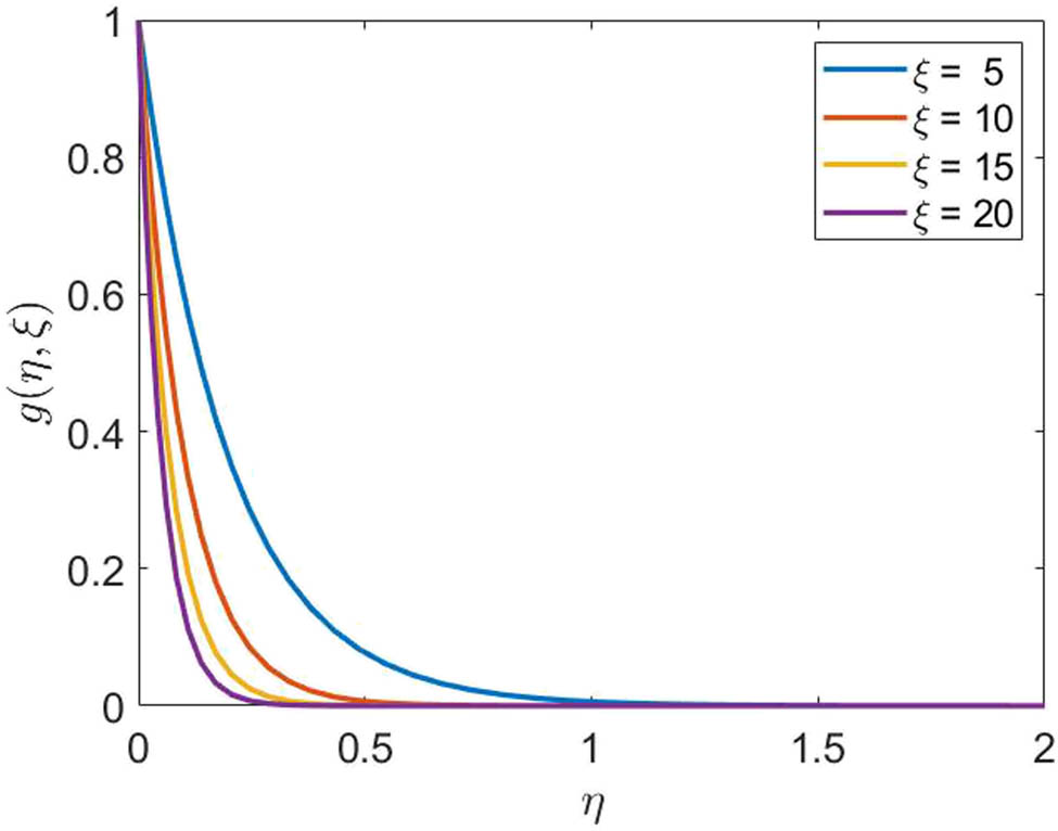
Figures 8 and 9 show that the errors for f ( ξ , η ) do not deteriorate for the values of n = 0 , 0.5 , 0.8 , 1 , and the values of n > 1 leads to the divergence of the numerical method used, this is consistent with the values used in ref. [25]. The values of ε are also admitted up to 0.9, which is consistent with the values used in ref. [10]. Values more than this would mean a large spinning velocity resulting in the divergence of solutions of f ( ξ , η ) .

$Figure 9 Effect of varying ε \varepsilon on E f {E}_{f} for ε 0 = 0.5 {\varepsilon }_{0}=0.5 , K p = 0.7 Kp=0.7 , Pr = Ec = 1 {\rm{\Pr }}={\rm{Ec}}=1 .$

Figure 9

Effect of varying ε on E f for ε 0 = 0.5 , K p = 0.7 , Pr = Ec = 1 .

Figures 10 and 11 depict that the errors for g ( ξ , η ) do not fluctuate for the values of n = 0 , 0.5 , 0.8 , 1 , and the values of n > 1 leads to the divergence of the numerical method used. The values of ε are also admitted up to 0.9. Increasing ε results in less fluctuations in the errors with increasing iterations for the solutions of g ( ξ , η ) .

$Figure 10 Effect of varying n n on E g {E}_{g} for ε = 0.5 \varepsilon =0.5 , ε 0 = 0.5 {\varepsilon }_{0}=0.5 , K p = 0.7 Kp=0.7 , Pr = Ec = 1 {\rm{\Pr }}={\rm{Ec}}=1 .$

Figure 10

Effect of varying n on E g for ε = 0.5 , ε 0 = 0.5 , K p = 0.7 , Pr = Ec = 1 .

$Figure 11 Effect of varying ε \varepsilon on E g {E}_{g} for ε 0 = 0.5 {\varepsilon }_{0}=0.5 , K p = 0.7 Kp=0.7 , Pr = Ec = n = 1 {\rm{\Pr }}={\rm{Ec}}=n=1 .$

Figure 11

Effect of varying ε on E g for ε 0 = 0.5 , K p = 0.7 , Pr = Ec = n = 1 .

In Figures 12–13, the error graphs for θ ( η , ξ ) show that the error does not change much with the increase in the temperature exponent parameter n and the spin parameter ε as iterations increase. This shows the stability and accuracy of the MD-BSQLM.

$Figure 12 Effect of varying n n on E θ {E}_{\theta } for ε = 0.5 , ε 0 = 0.5 \varepsilon =0.5,{\varepsilon }_{0}=0.5 , K p = 0.7 Kp=0.7 , Pr = Ec = 1 {\rm{\Pr }}={\rm{Ec}}=1 .$

Figure 12

Effect of varying n on E θ for ε = 0.5 , ε 0 = 0.5 , K p = 0.7 , Pr = Ec = 1 .

$Figure 13 Effect of varying n n on E θ {E}_{\theta } for ε = 0.5 \varepsilon =0.5 , ε 0 = 0.5 {\varepsilon }_{0}=0.5 , K p = 0.7 Kp=0.7 , Pr = Ec = 1 {\rm{\Pr }}={\rm{Ec}}=1 .$

Figure 13

Effect of varying n on E θ for ε = 0.5 , ε 0 = 0.5 , K p = 0.7 , Pr = Ec = 1 .

5 Conclusion

A spinning cone with variable surface temperature, suction and pressure work effect was considered. A system of PDEs describing the fluid flow around a spinning cone was solved using the MD-BSQLM. The numerical method was shown to be robust and accurate by comparison with other results obtained in the literature. Considering more domains makes this method unique and accurate. The method can be preferred in solving PDEs arising in fluid flow with large parameters.

The effects of increasing the suction parameter involving large values resulted in the decrease of velocity, spin velocity and temperature profiles. The errors for all the solutions for f ( ξ , η ) , g ( ξ , η ) and θ ( ξ , η ) did not deteriorate with increasing iterations for larger values of the suction parameter ξ . Increasing the surface temperature exponent and the spin parameter showed that the errors for the solutions of f ( ξ , η ) , g ( ξ , η ) and θ ( ξ , η ) did not change much with increasing iterations. Using more than one domain results in accurate results. This shows that the MD-BSQLM is robust and accurate. This method can be recommended for use in PDEs arising in fluid flow with large parameters.

Conflict of interest: Authors state no conflict of interest.

References

[1] Makarytchev SV, Langrish TAG, Fletcher DF. Exploration of spinning cone column capacity and mass transfer performance using CFD. Chem Eng Res Des. 2016;83:1372–80. 10.1205/cherd.03413Suche in Google Scholar

[2] Makinde OD. Entropy-generation analysis for variable-viscosity channel flow with non-uniform wall temperature. Appl. Energy. 2008;85:384–93. 10.1016/j.apenergy.2007.07.008Suche in Google Scholar

[3] Andrew D, Rees S, Bassom AP. Unsteady thermal boundary layer flows of a Bingham fluid in a porous medium following a sudden change in surface heat flux. Int J Heat Mass Transf. 2016;93:1100–6. 10.1016/j.ijheatmasstransfer.2015.10.021Suche in Google Scholar

[4] Asghar S, Mohyuddin R, Hayat T. Unsteady Flow of a Third-grade fluid in the case of suction. Math Comput Model. 2003;38:201–8. 10.1016/S0895-7177(03)90016-1Suche in Google Scholar

[5] Cloete M, Smit GJF. Analytical modelling and numerical verification of non-Newtonian fluid flow through and over two-dimensional porous media. J. Nonnewton Fluid Mech. 2016;227:1–16. 10.1016/j.jnnfm.2015.11.001Suche in Google Scholar

[6] Silva RA, Assato M, Marcelo de Lemos JS. Mathematical modelling and numerical results of power-law fluid flow over a finite porous medium. Int J Therm Sci. 2016;100:126–37. 10.1016/j.ijthermalsci.2015.09.019Suche in Google Scholar

[7] Cheng CY. Natural convection boundary layer flow of a micro-polar fluid over a vertical permeable cone with variable wall temperature. Int Commun Heat Mass Transf. 2011;38:429–33. 10.1016/j.icheatmasstransfer.2010.12.021Suche in Google Scholar

[8] Altun A, Bilir S, Ates A. Transient conjugated heat transfer in thermally developing laminar flow in thick walled pipes and mini-pipes with time periodically varying wall temperature boundary condition. Int J Heat Mass Transf. 2016;92:643–57. 10.1016/j.ijheatmasstransfer.2015.09.011Suche in Google Scholar

[9] Ashari A, Tafreshi HV. A two-scale modelling of motion-induced fluid release from thin fibrous porous media. Chem Eng Sci. 2009;64:2067–75. 10.1016/j.ces.2009.01.048Suche in Google Scholar

[10] Ece MC. Free convection flow about a vertical spinning cone under a magnetic field. Appl Math Computat. 2006;179:231–42. 10.1016/j.amc.2005.11.099Suche in Google Scholar

[11] Haddout Y, Mekheimer SKh, Mohamed MS. The extended Graetz problem for a gaseous slip flow in micropipe and parallel-plate micro-channel with heating section of finite length: Effects of axial conduction, viscous dissipation and pressure work. Int J Heat Mass Transf. 2015;80:673–87. 10.1016/j.ijheatmasstransfer.2014.09.064Suche in Google Scholar

[12] Javaherdeh K, Nejad MM, Moslemi M. Natural convection heat and mass transfer in MHD fluid flow pasta moving vertical plate with variable surface temperature and concentration in a porous medium. Eng Sci Technol Int. 2015;18:423–31. 10.1016/j.jestch.2015.03.001Suche in Google Scholar

[13] Kefayati GHR. Simulation of double diffusive natural convection and entropy generation of power-law fluids in an inclined porous cavity with Soret and Dufour effects (Part I: Study of fluid flow, heat and mass transfer). Int J Heat Mass Transf. 2016;94:539–81. 10.1016/j.ijheatmasstransfer.2015.11.044Suche in Google Scholar

[14] Rosali H, Ishak A, Pop I. Micro-polar fluid flow towards a stretching/shrinking sheet in a porous medium with suction. Int Commun Heat Mass Transf. 2016;39:826–9. 10.1016/j.icheatmasstransfer.2012.04.008Suche in Google Scholar

[15] Teymourtash AR, Khonakdar DR, Raveshi MR. Natural convection on a vertical plate with variable heat flux in supercritical fluids. J Supercrit Fluids. 2016;74:115–27. 10.1016/j.supflu.2012.12.010Suche in Google Scholar

[16] Dinarvand S, Saber M, Aulhasansari M. Micro-polar fluid flow and heat transfer about a spinning cone with Hall current and Ohmic heating. J Mech Eng Sci. 2014;228:1900–12. 10.1177/0954406213512628Suche in Google Scholar

[17] Turkyilmazoglu M. Analytic approximate solutions of rotating disk boundary layer flow subject to a uniform suction or injection. Int J Mech Sci. 2010;52:1735–44. 10.1016/j.ijmecsci.2010.09.007Suche in Google Scholar

[18] Abd Elmaboud Y, Lahjomri J, Mohamed MS. Series solution of a natural convection flow for a Carreau fluid in a vertical channel with peristalsis. J Hydrodynam B. 2015;6:696–979. 10.1016/S1001-6058(15)60559-5Suche in Google Scholar

[19] Haque MZ, Alam MM, Ferdows M. Micro-polar fluid behaviours on steady MHD free convection and mass transfer flow with constant heat and mass fluxes, joule heating and viscous dissipation. J King Saud Univ Eng Sci. 2012;24:71–84. 10.1016/j.jksues.2011.02.003Suche in Google Scholar

[20] Markicevic B, Hoff K, Li H, Zand AR, Navaz HK. Capillary force driven primary and secondary unidirectional flow of wetting liquid into porous medium. Int J Multiph Flow. 2012;39:193–204. 10.1016/j.ijmultiphaseflow.2011.09.008Suche in Google Scholar

[21] Pinar E, Ozkan GM, Durhasan T, Aksoy MM, Akilli H, Sahin B. Flow structure around perforated cylinders in shallow water. J. Fluid Struct. 2015;55:52–63. 10.1016/j.jfluidstructs.2015.01.017Suche in Google Scholar

[22] Magagula VM, Motsa SS, Sibanda P. Multidomain bivariate pseudo-spectral quasilinearization method for systems of nonlinear partial differential equations. Comp Math Methods. 2020;2:e1096, 10.1002/cmm4.1096. Suche in Google Scholar

[23] Motsa SS, Dlamini PG, Khumalo M. Spectral relaxation method and spectral quasilinearization method for solving unsteady boundary layer flow problems. Adv Math Phys. 2014;2014:Article ID 341964, 12 pages, 10.1155/2014/341964. Suche in Google Scholar

[24] Motsa SS, Sibanda P. On extending the quasilinearization method to higher order convergent hybrid schemes using the spectral homotopy analysis method. J Appl Math. 2013;2013:Article ID 879195, 9 pages, 10.1155/2013/879195. Suche in Google Scholar

[25] Alim MA, Alam MM, Chowdhury MMK. Pressure work effect on natural convection flow from a vertical circular cone with suction and a non-uniform surface temperature. J Mech Eng. 2006;ME36:6–11. 10.3329/jme.v36i0.805Suche in Google Scholar

[26] Makanda G, Sibanda P, Makinde OD. Natural convection of viscoelastic fluid from a cone embedded in a porous medium with viscous dissipation. Math Probl Eng. 2013;14:1–11, 10.1155/2013/934712. Suche in Google Scholar

Received: 2020-07-29

Revised: 2020-09-07

Accepted: 2020-09-30

Published Online: 2021-04-16

This work is licensed under the Creative Commons Attribution 4.0 International License.

Artikel in diesem Heft

https://doi.org/10.1515/phys-2020-0189

Schlagwörter für diesen Artikel

numerical analysis; spectral methods; multi-domain; error analysis

Creative Commons

BY 4.0