Time-periodic pulse electroosmotic flow of Jeffreys fluids through a microannulus

Dongsheng Li; Liang Ma; Jiayin Dong; Kun Li

doi:10.1515/phys-2021-0106

Article Open Access

Time-periodic pulse electroosmotic flow of Jeffreys fluids through a microannulus

Dongsheng Li , Liang Ma , Jiayin Dong and Kun Li

Published/Copyright: December 31, 2021

Published by

Become an author with De Gruyter Brill

Submit Manuscript Author Information Explore this Subject

From the journal Open Physics Volume 19 Issue 1

Abstract

In this article, we investigate the time-periodic pulse electroosmotic flow (EOF) of Jeffreys fluids through a microannulus. By using the Laplace transform method, the velocity expression of the pulse EOF is derived. The effect of some variables on the time it takes for the fluid to go from a static state to a flowing state is analyzed. We find that increasing the relaxation time λ ¯ 1 and decreasing the inner and outer radius ratio α will result in longer time for the fluid to reach the flowing state, but the retardation time λ ¯ 2 and the inner and outer zeta potential ratio β have little effect on it. The impact of some related parameters on the pulse EOF velocity for different inner and outer radius ratios ( α ) is discussed in detail. The results show that for a smaller inner and outer radius ratio α , the velocity amplitude increases with the relaxation time λ ¯ 1 and decreases with the retardation time λ ¯ 2 . As the inner and outer radius ratio α increases, the effect of relaxation time λ ¯ 1 on velocity amplitude gradually weakens or even becomes insignificant, and the effect of the retardation time λ ¯ 2 on the velocity amplitude remains unchanged. Moreover, the velocity amplitude will decrease with the increase in the inner and outer radius ratio α and its change range will expand from the electric double layer near the annular wall to the entire flow region.

Keywords: pulse electroosmotic flow; Laplace transform; Jeffreys fluids; microannulus

1 Introduction

In the past few decades, because of the rapid development of microfluidic devices and their innovative applications in the microelectromechanical system and microbiological sensors such as lab-on-a-chip [1,2], the electroosmosis flow (EOF) has become an interesting topic among researchers. The principle of the EOF is explained as follows. In general, when most substances come into contact with polar solutions, they tend to generate negative charges on the surface. The distribution of ions close to the wall in the solution will be affected by this phenomenon. The ions with opposite polarity to the wall will be attracted to the wall, while the same ions will be repelled away from the wall. In this way, an electric double layer (EDL) will be formed [3]. Furthermore, when an external electric field is applied to both ends of the channel, the ions in the EDL will move under the electric field force. This is mainly due to the viscosity of the fluid itself, which causes the moving free ions to drive the movement of the nearby fluid mass, ultimately forming an EOF. At present, the EOF has become increasingly important owing to its operational advantages, like plug flow type behavior, absence of mechanical pumping equipment and better flow control [4].

By viewing the existing literature studies, a large number of theoretical and experimental studies on the fully developed EOF of the Newtonian fluids in microchannels under different geometric domains and physical conditions have been found [5,6,7,8]. Very recently, the time-dependent EOF as an alternative mechanism of microfluidic transport has attracted increasing attention from many researchers [9,10,11,12].

Although we know from the above-mentioned literature studies that many constructive results have been achieved in the study of Newtonian fluids, there are many applications of fluids with non-Newtonian fluid structure characteristics in actual situations. Especially in the biomedical field where microfluidic devices are widely used, many biological fluids such as blood, saliva and DNA solutions are essentially viscoelastic, and blood viscoelasticity is a useful clinical parameter. Since biological fluids are conductive in nature, electroosmotic flow is also very important for drug delivery and separation and mixing at the atomic level. These biological fluids are usually simulated with non-Newtonian fluid models such as Maxwell fluids model, Phan-Thien-Tanner fluids model, Burgers fluids model, Jeffreys fluids model, Oldroyd-B fluids model, etc. Unlike Newtonian fluids, the shear stress and flow field of non-Newtonian fluids are relatively more complex. Hence, we can use the more general Cauchy momentum equation to replace the Navier–Stokes equation to describe its complex motion model [13]. Some more work related to the current study on non-Newtonian fluids can be seen in references [14–19].

The Jeffreys fluid model, as a typical non-Newtonian fluid model, has received special attraction from researchers due to its wide application in biology, industry, and other fields. In this fluid model, the two parameters λ 1 and λ 2 describe the behavior of the relaxation and retardation times, respectively [20]. If these two parameters take specific values, the Jeffreys fluid model can be degenerated into two classical fluid models, for instance, the Newtonian fluids model ( λ 1 = λ 2 = 0 ) and the Maxwell fluids model ( λ 1 ≠ 0, λ 2 = 0 ) [21]. In particular, a recent study [22] has found that the Jeffreys fluid model was used to simulate blood flow through a narrowed tapered artery, and the blood and other biofluids are usually analyzed by electrokinetic mechanisms in blood-based microfluidic transmission systems. Therefore, it is very important to carry out more in-depth research on Jeffreys fluids. For recent various studies on Jeffreys fluids, see references [23–30].

However, to the best of our knowledge, until now, research on pulse EOF of Jeffreys fluids has not been discovered much. Also, taking into account the wide application of pulse current (PC) in materials engineering in recent years [31,32], combined with the remarkable advantages of the annular channel (for instance, compact structure, large heat transfer area, good fluidity, and high heat transfer coefficient), the main purpose of this article is to study the time-periodic pulse EOF of Jeffreys fluids through a microannulus. The semi-analytical expression of velocity is obtained and the influence of some parameters on it is discussed.

2 Problem formulation

2.1 Cauchy momentum equation and constitutive relation

Consider the time-periodic pulse EOF of incompressible viscoelastic fluids through an annular region with an inner radius α R ( 0 < α < 1 ) and outer radius R ; the length of the channel is L , and is assumed to be much larger than the radius R (i.e. L ≫ R ), as shown in Figure 1 [33]. Introduce a two-dimensional coordinate system, where the r - and z -axis are the radical and flow of the fluid’s direction, respectively. The pulse EOF is pumped by a PC electric field of strength E 0 applied in the z -axis direction. It should be mentioned here that the viscoelastic fluids and pulse are described by Jeffreys fluids and rectangle pulse, respectively. The rectangle pulse is defined by a rectangle square wave with a pulse amplitude of 1, a pulse repetition period of 2a, and a pulse width of a (see Figure 2), and can be expressed as

(1) f ( t ) = 1 , t ∈ [ 0 , a ) , − 1 , t ∈ ( a , 2 a ] .

Figure 1

(a) Sketch of the time-periodic pulse EOF of Jeffreys fluids through a microannulus. (b) Cross-section of the microannulus.

Figure 2

Schematic of the rectangle pulse wave.

If we assume that any external pressure gradient and gravity effects are ignored, the one-dimensional momentum equation can be given by

(2) ρ ∂ u ( r , t ) ∂ t = − 1 r ∂ ∂ r ( r τ r z ) + ρ e ( r ) E 0 f ( t ) ,

where u ( r , t ) is the velocity along the z-axis direction, ρ is the fluid density, t is the time, and τ r z and ρ e ( r ) are the stress tensor and the volume charge density, respectively.

Generally speaking, the transient relaxation effect of the EDL can be neglected. The reason is that the time scale related to electromigration in the EDL is at least two orders smaller than the characteristic time associated with the evolution of the pulse EOF and also much less than the relaxation time of the viscoelastic fluids [34]. If we further assume that the boundary conditions of equation (2) are no-slip, then the no-slip and the initial condition can be written as [16,33]

(3) u ( r , t ) | r = R = 0 , u ( r , t ) | r = α R = 0 ,

(4) u ( r , t ) | t = 0 = 0 , ∂ u ( r , t ) ∂ t t = 0 = 0 .

For the Jeffreys fluids, its constitutive equation satisfies the following form [35]:

(5) τ r z + λ 1 ∂ ∂ t τ r z = − η 0 1 + λ 2 ∂ ∂ t ∂ u ( r , t ) ∂ r ,

where λ 1 is the relaxation time, λ 2 is the retardation time, and η 0 is the zero shear rate viscosity.

2.2 Electric potential field solution

For a symmetrical low-concentration binary electrolyte solution and the thin EDL, the net charge density is governed by the Poisson–Boltzmann equations

(6) 1 r d d r r d ψ ( r ) d r = − ρ e ( r ) ε ,

(7) ρ e ( r ) = z ν e 0 ( n + − n − ) = − 2 n 0 z ν e 0 sinh z ν e 0 ψ ( r ) k B T ,

where ψ ( r ) is the electrical potential of the EDL, ε is the dielectric constant of the electrolyte liquid, z ν is the valence number of ions, n 0 is the ion density of the bulk liquid, e 0 is the electron charge, and k B and T are the Boltzmann constant and the absolute temperature, respectively.

Combining equations (6) and (7), the electrical potential in the annular region can be derived as

(8) 1 r d d r r d ψ ( r ) d r = 2 n 0 z ν e 0 ε sinh z ν e 0 ψ ( r ) k B T .

This equation is subject to the following boundary conditions:

(9) ψ ( r ) | r = R = ς 0 , ψ ( r ) | r = α R = ς i ,

where ς 0 and ς i are the outer and inner capillary wall zeta potentials, respectively.

The following dimensionless groups are introduced:

(10) r ¯ = r R , K = κ R , κ = 2 n 0 z ν 2 e 0 2 ε k B T 1 / 2 , [ ψ ( r ¯ ) ¯ , ς 0 ¯ , ς i ¯ ] = z ν e 0 k B T [ ψ ( r ) , ς 0 , ς i ] ,

where κ is the Debye–Hückel parameter and K is the dimensionless electrokinetic width.

Provided that the wall potentials are axially invariant and low enough ( ∣ ψ ∣ ≤ 25 mV ), we can apply the Debye–Hückel approximation in equation (8) and with the aid of dimensionless groups (10), the electrical potential (8) and its corresponding boundary conditions (9) can be simplified as

(11) 1 r ¯ d d r ¯ r d ψ ( r ¯ ) ¯ d r ¯ = K 2 ψ ( r ¯ ) ¯ ,

(12) ψ ( r ¯ ) ¯ | r ¯ = 1 = ς 0 ¯ , ψ ( r ¯ ) ¯ | r ¯ = α = ς i ¯ ,

We notice that equation (11) is a modified Bessel equation, so its solution can be written as

(13) ψ ( r ¯ ) ¯ = A ′ I 0 ( K r ¯ ) + B ′ K 0 ( K r ¯ ) ,

here I 0 and K 0 are the zero-order modified Bessel functions of the first and second types, respectively.

By using equation (12) to solve equation (13), the coefficients A ′ and B ′ can be determined by

(14) A ′ = K 0 ( K α ) ς 0 ¯ − K 0 ( K ) ς i ¯ K 0 ( K α ) I 0 ( K ) − K 0 ( K ) I 0 ( K α ) , B ′ = I 0 ( K α ) ς 0 ¯ − I 0 ( K ) ς i ¯ K 0 ( K ) I 0 ( K α ) − K 0 ( K α ) I 0 ( K ) .

The solution of the electric potential field can be derived by integrating equations (13) and (14)

(15) ψ ( r ¯ ) ¯ = ς 0 ¯ [ A I 0 ( K r ¯ ) + B K 0 ( K r ¯ ) ] ,

where

(16) A = K 0 ( K α ) − β K 0 ( K ) K 0 ( K α ) I 0 ( K ) − K 0 ( K ) I 0 ( K α ) , B = I 0 ( K α ) − β I 0 ( K ) K 0 ( K ) I 0 ( K α ) − K 0 ( K α ) I 0 ( K ) ,

with β = ς i / ς 0 being defined as the ratio of the zeta potentials of the inner wall to the outer wall of the microannulus. It needs to be further expanded here that if α = β = 0 , it means that the EDL of the pulse EOF is in the circular microchannel. At this time, I 0 ( 0 ) = 0 and K 0 ( 0 ) = ∞ ; thus, equation (16) becomes A = 1 / I 0 ( K ) , B = 0 ; the corresponding electric field potential (15) is exactly the same as that of the circular microchannel [36].

Finally, the charge density can be obtained by solving equation (11) with boundary conditions (12):

(17) ρ e ( r ) = − 2 n 0 z ν e 0 ψ ( r ¯ ) ¯ = − ε κ 2 ς 0 [ A I 0 ( K r ¯ ) + B K 0 ( K r ¯ ) ] .

2.3 Velocity field solution

In order to solve the velocity field, some dimensionless variables are defined as

(18) u ¯ ( r ¯ , t ¯ ) = u ( r , t ) U eo , τ r z ¯ ¯ = τ r z η 0 U eo / R , ( a ¯ , t ¯ , λ ¯ 1 , λ ¯ 2 ) = ( a , t , λ 1 , λ 2 ) ρ R 2 / η 0 ,

where U eo = − ε ς 0 E 0 / η 0 denotes the steady Helmholtz–Smoluchowshi EOF velocity of Newtonian fluids. Applying equation (18), equations (2) and (5) and conditions (3)–(4) are normalized as

(19) ∂ u ¯ ( r ¯ , t ¯ ) ∂ t ¯ = − 1 r ¯ ∂ ∂ r ¯ ( r ¯ τ r z ¯ ¯ ) + f ( t ¯ ) K 2 [ A I 0 ( K r ¯ ) + B K 0 ( K r ¯ ) ] ,

(20) τ r z ¯ ¯ + λ ¯ 1 ∂ ∂ t ¯ τ r z ¯ ¯ = − 1 + λ ¯ 2 ∂ ∂ t ¯ ∂ u ¯ ( r ¯ , t ¯ ) ∂ r ¯ ,

(21) u ¯ ( r ¯ , t ¯ ) | r ¯ = 1 = 0 , u ¯ ( r ¯ , t ¯ ) | r ¯ = α = 0 ,

(22) u ¯ ( r ¯ , t ¯ ) | t ¯ = 0 = 0 , ∂ u ¯ ( r ¯ , t ¯ ) ∂ t ¯ t ¯ = 0 = 0 .

Eliminating the dimensionless stress tensor τ r z ¯ ¯ from equations (19) and (20) yields

(23) 1 + λ ¯ 2 ∂ ∂ t ¯ ∂ 2 u ¯ ( r ¯ , t ¯ ) ∂ r ¯ 2 + 1 r ¯ ∂ u ¯ ( r ¯ , t ¯ ) ∂ r ¯ − 1 + λ ¯ 1 ∂ ∂ t ¯ ∂ u ¯ ( r ¯ , t ¯ ) ∂ t ¯ = − 1 + λ ¯ 1 ∂ ∂ t ¯ f ( t ¯ ) K 2 [ A I 0 ( K r ¯ ) + B K 0 ( K r ¯ ) ] .

Let us employ the method of Laplace transform defined by

(24) U ( r ¯ , s ) = L [ u ¯ ( r ¯ , t ¯ ) ] = ∫ 0 ∞ u ¯ ( r ¯ , t ¯ ) e − s t ¯ d t ¯ .

With the help of the initial condition (22), the transforms of equation (23) and boundary conditions (21) can be rewritten as

(25) ∂ 2 U ( r ¯ , s ) ∂ r ¯ 2 + 1 r ¯ ∂ U ( r ¯ , s ) ∂ r ¯ − γ 2 U ( r ¯ , s ) = − tanh ( a ¯ s / 2 ) ( 1 + λ ¯ 2 s ) s K 2 [ A I 0 ( K r ¯ ) + B K 0 ( K r ¯ ) ] ,

(26) U ( r ¯ , s ) | r ¯ = 1 = 0 , U ( r ¯ , s ) | r ¯ = α = 0 ,

where γ = ( 1 + λ ¯ 1 s ) s / ( 1 + λ ¯ 2 s ) . It is clear that equation (25) is a linear and inhomogeneous ordinary differential equation, and thus, the solution of equation (25) can be written as the sum of a homogeneous solution U h ( r ¯ , s ) and a particular solution U p ( r ¯ , s ) :

(27) U ( r ¯ , s ) = U h ( r ¯ , s ) + U p ( r ¯ , s ) .

On the one hand, by solving the homogeneous equation (25), we can get

(28) U h ( r ¯ , s ) = C I 0 ( γ r ¯ ) + D K 0 ( γ r ¯ ) ,

where C and D are constants and can be determined from the boundary conditions of equation (26).

On the other hand, the particular solution is given by considering the variable form of the right-hand side of equation (25)

(29) U p ( r ¯ , s ) = E I 0 ( K r ¯ ) + F K 0 ( K r ¯ ) ,

where E and F are also constants. Inserting equations (29) into (25) yields

(30) E d 2 I 0 ( K r ¯ ) d r ¯ 2 + 1 r ¯ d I 0 ( K r ¯ ) d r ¯ − γ 2 I 0 ( K r ¯ ) + F d 2 K 0 ( K r ¯ ) d r ¯ 2 + 1 r ¯ d K 0 ( K r ¯ ) d r ¯ − γ 2 K 0 ( K r ¯ ) = − tanh ( a ¯ s / 2 ) ( 1 + λ ¯ 2 s ) s K 2 [ A I 0 ( K r ¯ ) + B K 0 ( K r ¯ ) ] .

From equation (11), we can obtain the following conclusions:

(31) d 2 I 0 ( K r ¯ ) d r ¯ 2 + 1 r ¯ d I 0 ( K r ¯ ) d r ¯ = K 2 I 0 ( K r ¯ ) , d 2 K 0 ( K r ¯ ) d r ¯ 2 + 1 r ¯ d K 0 ( K r ¯ ) d r ¯ = K 2 K 0 ( K r ¯ ) .

After substituting equation (31) into equation (30), and equalizing the coefficients in front of the modified Bessel functions I 0 and K 0 on the two sides of the equation, we have

(32) E = − A K 2 tanh ( a ¯ s / 2 ) ( K 2 − γ 2 ) ( 1 + λ ¯ 2 s ) s , F = − B K 2 tanh ( a ¯ s / 2 ) ( K 2 − γ 2 ) ( 1 + λ ¯ 2 s ) s .

Therefore, the solution of the velocity U ( r ¯ , s ¯ ) can be expressed as

(33) U ( r ¯ , s ) = C I 0 ( γ r ¯ ) + D K 0 ( γ r ¯ ) + E I 0 ( K r ¯ ) + F K 0 ( K r ¯ ) .

The coefficients C and D with boundary conditions of equation (26) can be determined as

(34) C = K 0 ( γ α ) [ E I 0 ( K ) + F K 0 ( K ) ] − K 0 ( γ ) [ E I 0 ( K α ) + F K 0 ( K α ) ] I 0 ( γ α ) K 0 ( γ ) − I 0 ( γ ) K 0 ( γ α ) , D = I 0 ( γ α ) [ E I 0 ( K ) + F K 0 ( K ) ] − I 0 ( γ ) [ E I 0 ( K α ) + F K 0 ( K α ) ] I 0 ( γ ) K 0 ( γ α ) − I 0 ( γ α ) K 0 ( γ ) .

The analytical solution of the Laplace transform of the time-periodic pulse EOF velocity through a microannulus is shown by equation (33) and the correlation coefficients are determined by equations (16), (32), and (34). Then, we use the method of inverse Laplace transform defined by

(35) u ¯ ( r ¯ , t ¯ ) = L − 1 [ U ( r ¯ , s ) ] = 1 2 π i ∫ Γ U ( r ¯ , s ) e s t ¯ d s ,

where Γ is a vertical line to the right of all singularities of U ( r ¯ , s ) in the complex s plane. The numerical inversion must be performed by the numerical inverse Laplace transform [37] method because of the complexity of the expression U ( r ¯ , s ) .

3 Results and discussion

Although the important results of our work on dimensionless parameters have been presented in the above section, we still need to point out some typical values of the corresponding dimensional parameters when solving practical engineering problems. The typical parameter values are given as follows [13,36]: 0 < α < 1 , ρ = 10³ kg m⁻³, η ₀ = 10⁻³kg m⁻¹s⁻¹, R = 100 μm, and 10 − 4 s ≤ λ 1 ≤ 10 3 s . Considering that the relaxation time is larger than the retardation time and it should be much smaller than the observation time (i.e. the period of the pulsed electric field), that is λ 2 < λ 1 < 2 a . Besides, the pulse EOF velocity in the center ( r ¯ = ( 1 + α ) / 2 ) of the annular microchannel is shown in Figures 3 and 7. In other words, when the inner to outer radius ratio α = 0.2, 0.4, 0.6, and 0.8, the corresponding radius r ¯ = 0.6, 0.7, 0.8, and 0.9, respectively. All symbols used in this work are defined in Table 1.

$Figure 3 Effects of the relaxation time when λ ¯ 2 = 0.1 {\bar{\lambda }}_{2}=0.1 , α = 0.2 \alpha =0.2 and β = 1 \beta =1 (a); the retardation time when λ ¯ 1 = 0.5 {\bar{\lambda }}_{1}=0.5 , α = 0.2 \alpha =0.2 , and β = 1 \beta =1 (b); the inner to outer radius ratio when λ ¯ 1 = 0.8 {\bar{\lambda }}_{1}=0.8 , λ ¯ 2 = 0.1 {\bar{\lambda }}_{2}=0.1 and β = 1 \beta =1 (c); the inner to outer wall zeta potential ratio when λ ¯ 1 = 0.2 {\bar{\lambda }}_{1}=0.2 , λ ¯ 2 = 0.1 {\bar{\lambda }}_{2}=0.1 and α = 0.2 \alpha =0.2 (d) on the pulse EOF velocity profiles of Jeffreys fluids when K = 20 K=20 and a ¯ = 1 \bar{a}=1 in the microannulus.$

Figure 3

Effects of the relaxation time when λ ¯ 2 = 0.1 , α = 0.2 and β = 1 (a); the retardation time when λ ¯ 1 = 0.5 , α = 0.2 , and β = 1 (b); the inner to outer radius ratio when λ ¯ 1 = 0.8 , λ ¯ 2 = 0.1 and β = 1 (c); the inner to outer wall zeta potential ratio when λ ¯ 1 = 0.2 , λ ¯ 2 = 0.1 and α = 0.2 (d) on the pulse EOF velocity profiles of Jeffreys fluids when K = 20 and a ¯ = 1 in the microannulus.

Table 1

List of symbols

Symbol	Meaning
e 0	Elementary electric charge (C)
E 0	Strength of the rectangle pulse electric field (V m⁻¹)
K	Dimensionless electrokinetic width
k B	Boltzmann constant (J K⁻¹)
T	Temperature of the fluid (K)
z v	Valence number of ions
n 0	Bulk volume concentration of the charge of positive or negative ions (m⁻³)
U e o	Helmholtz–Smoluchowski electroosmotic velocity (m s⁻¹)
R	Outer radius of the annular channel (m)
L	Length of the annular channel (m)
a	Pulse width of the rectangle pulse electric field (s)
a ¯	Dimensionless pulse width of the rectangle pulse electric field
u	Velocity field (m s⁻¹)
u ¯	Dimensionless velocity field in the axial direction
f ( t )	Time-periodic rectangle pulse function
I 0 , K 0	Zero-order-modified Bessel functions of first and second types
r , θ , z	Cylindrical polar coordinate components
ε	Fluid permittivity (C V⁻¹ m⁻¹)
ρ	Density (kg m⁻³)
η 0	Zero shear rate viscosity of the fluid (Pa s)
ρ e	Local volumetric net charge density (C m⁻³)
λ 1	Relaxation time of the fluid (s)
λ 1 ¯	Dimensionless relaxation time of the fluid
ψ	Electrical potential (V)
ψ ¯	Dimensionless electrical potential
ζ 0 , ζ i	Zeta potential of the outer and inner capillary wall (V)
ζ 0 ¯ , ζ i ¯	Dimensionless zeta potential of the outer and inner capillary wall
α , β	Inner to outer radius ratio and inner to outer wall zeta potential ratio

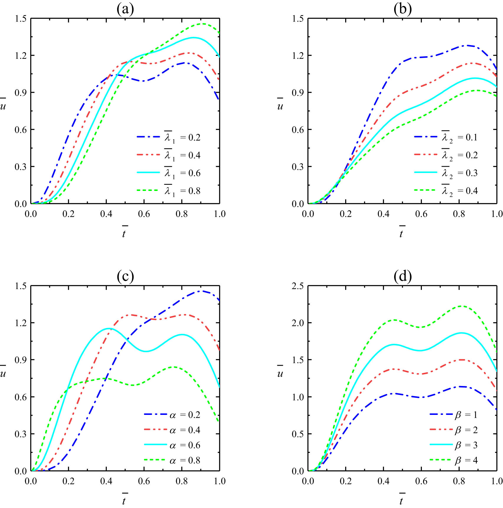
It is well known that studying the time required for the fluid to change from a static state to a flowing state is a very important aspect of pulse EOF research. The effects of some variables (such as the relaxation time λ ¯ 1 , the retardation time λ ¯ 2 , the inner to outer radius ratio α , and the inner to outer wall zeta potential ratio β ) on the velocity profiles are presented in Figure 3. From the above figures, we can easily see that increasing the relaxation time λ ¯ 1 and decreasing the inner and outer radius ratio α will lead to the fluid taking longer time to reach the flowing state. The main reason for this fact is that longer relaxation time λ ¯ 1 means larger elastic effect and weaker recovery ability of the Jeffreys fluids, which results in the pulse EOF velocity profiles changing easily under the action of an external electric field [38]. For a smaller inner and outer radius ratio α , there is a larger gap between the two microannulus walls, and the fluid flow region is relatively larger, so the longer it takes for the fluid to reach the flowing state. In addition, no matter how the retardation time λ ¯ 2 and the inner to outer wall zeta potential ratio β increase, they have little effect on the time required for the fluid to reach the flowing state (see Figure 3(b) and (d)).

Figures 4–7 depict the effects of several related parameters on the velocity profiles for different inner and outer radius ratios ( α ), respectively. On the whole, with the increase of the inner and outer radius ratio α , the velocity amplitude decreases and its variation range begins to expand to the entire region of the flow instead of being confined to the EDL near the two annular walls (see Figure 4(b), 5(b) and 6(b)). The reason is that a larger α value means that a smaller gap between the two annular walls, namely, a narrower flow area, thus the velocity amplitude will be reduced and the velocity variation will be relatively faster to expand to the entire flow field. It can be observed from Figure 4 that when the α value is smaller, the velocity amplitude increases with the increase of relaxation time λ ¯ 1 , but this effect will become extremely insignificant for a larger α value. This implies that the reduction of the wall gap will restrict the elastic effect of the fluid. More interestingly, we can see from Figure 5 that the velocity amplitude decreases as the retardation time λ ¯ 2 gradually increases due to the suppression effect of the retardation time, and this result is not affected by the α values.

$Figure 4 Variations of the pulse EOF velocity at different relaxation times λ ¯ 1 {\bar{\lambda }}_{1} with the radius for different inner to outer radius ratios ( α \alpha ) when K = 20 K=20 , λ ¯ 2 =0 .1 {\bar{\lambda }}_{\text{2}}\text{=0}\text{.1} , t ¯ = 0.8 \bar{t}=0.8 , a ¯ = 1 \bar{a}=1 and β = 1 \beta =1 . (a) α = 0.2 \alpha =0.2 and (b) α = 0 . 8 \alpha =0.\text{8} .$

Figure 4

Variations of the pulse EOF velocity at different relaxation times λ ¯ 1 with the radius for different inner to outer radius ratios ( α ) when K = 20 , λ ¯ 2 =0 .1 , t ¯ = 0.8 , a ¯ = 1 and β = 1 . (a) α = 0.2 and (b) α = 0 . 8 .

$Figure 5 Variations of the pulse EOF velocity at different retardation times λ ¯ 2 {\bar{\lambda }}_{2} with the radius for different inner to outer radius ratios ( α \alpha ) when K = 20 K=20 , λ ¯ 1 =0 .5 {\bar{\lambda }}_{\text{1}}\text{=0}\text{.5} , t ¯ = 0.8 \bar{t}=0.8 , a ¯ = 1 \bar{a}=1 and β = 1 \beta =1 . (a) α = 0.2 \alpha =0.2 and (b) α = 0 . 8 \alpha =0.\text{8} .$

Figure 5

Variations of the pulse EOF velocity at different retardation times λ ¯ 2 with the radius for different inner to outer radius ratios ( α ) when K = 20 , λ ¯ 1 =0 .5 , t ¯ = 0.8 , a ¯ = 1 and β = 1 . (a) α = 0.2 and (b) α = 0 . 8 .

$Figure 6 Variations of the pulse EOF velocity at different inner to outer wall zeta potential ratios ( β \beta ) with the radius for different inner to outer radius ratios ( α \alpha ) when K = 20 K=20 , λ ¯ 1 = 0.2 {\bar{\lambda }}_{1}=0.2 , λ ¯ 2 = 0.1 {\bar{\lambda }}_{2}=0.1 , t ¯ = 0.8 \bar{t}=0.8 , and a ¯ = 1 \bar{a}=1 . (a) α = 0.2 \alpha =0.2 and (b) α = 0 . 8 \alpha =0.\text{8} .$

Figure 6

Variations of the pulse EOF velocity at different inner to outer wall zeta potential ratios ( β ) with the radius for different inner to outer radius ratios ( α ) when K = 20 , λ ¯ 1 = 0.2 , λ ¯ 2 = 0.1 , t ¯ = 0.8 , and a ¯ = 1 . (a) α = 0.2 and (b) α = 0 . 8 .

$Figure 7 Variations of the pulse EOF velocity at different pulse widths a ¯ \bar{a} with time for different inner to outer radius ratios ( α \alpha ) when K = 20 K=20 , λ ¯ 1 = 0.2 {\bar{\lambda }}_{1}=0.2 , λ ¯ 2 = 0.1 {\bar{\lambda }}_{2}=0.1 , and β = 1 \beta =1 . (a) α = 0.2 \alpha =0.2 and (b) α = 0 . 8 \alpha =0.\text{8} .$

Figure 7

Variations of the pulse EOF velocity at different pulse widths a ¯ with time for different inner to outer radius ratios ( α ) when K = 20 , λ ¯ 1 = 0.2 , λ ¯ 2 = 0.1 , and β = 1 . (a) α = 0.2 and (b) α = 0 . 8 .

The impact of the inner to outer wall zeta potential ratio β on the velocity profiles of pulse EOF is illustrated in Figure 6. As expected, it can be found from Figure 6 that the magnitude and direction of the pulse EOF velocity are determined by the β value. The pulse EOF velocity directions of the EDL near the wall of the two annular microchannels are opposite when the β value is negative. On the contrary, the directions are the same for a positive β value. Larger β value causes larger velocity in the area near the inner wall of the microannulus. The main reason is that most of the electric field force determined by the electric potential is concentrated on the EDL close to the annular wall, and the inner and outer wall zeta potential is affected by the β value, so the β value can indirectly determine the magnitude of velocity. The above conclusions agree well with those obtained in references [33,36].

The variations of the pulse EOF velocity with time for different pulse widths a ¯ are shown in Figure 7. It is evident that no matter what value the pulse width a ¯ is, the velocity profiles tend to a steady state over time, and the change in velocity is not significant at this time. It should be clarified here that the value of change is only of a small order of magnitude, but not really zero, and it does not mean that the fluid flow is stationary either. This phenomenon can be explained by the fact that the effect of the electric field force on the fluid is a process that gradually weakens with time, which is also one of the characteristics of the unsteady EOF. The larger the pulse width a ¯ , the longer it requires for the velocity profiles to attain the steady state. This may be because a larger pulse width a ¯ means that the pulse force has a relatively long duration in orientation.

4 Conclusion

A semi-analytical solution of the time-periodic pulse EOF of Jeffreys fluids in a microannulus under the Debye–Hückel approximation is presented in this work. The effects of some related parameters on pulse EOF velocity are investigated and the following conclusions can be drawn. Increasing the relaxation time λ ¯ 1 and decreasing the inner and outer radius ratio α will prolong the time for the fluid to reach the flowing state. However, the increase of the retardation time λ ¯ 2 and the inner to outer wall zeta potential ratio β have little effect on the time it takes for the fluid to reach the flowing state. For a given smaller α value, the velocity amplitude increases with λ ¯ 1 . But as the α value increases, this effect will gradually weaken and become no longer significant. The velocity amplitude decreases with the increase of the retardation time λ ¯ 2 , and the result is not affected by α . The magnitude and direction of the pulse EOF velocity are determined by the β value. When β takes a positive or negative value, the corresponding directions of the EDL near the wall of the two annular microchannels are the same or opposite, respectively. Larger β value results in larger velocity in the area near the inner microannulus wall. The velocity profiles tend to a steady state with time for any pulse width a ¯ . The larger the pulse width a ¯ , the longer it takes for the velocity profiles to reach a steady state. Furthermore, increasing the inner and outer radius ratio α will cause smaller velocity amplitude.

Acknowledgments

The author wishes to express his appreciation to the anonymous reviewers for their high-level comments and the kind editors for all their assistance.

Funding information: This work was supported by the Scientific Research Project of Inner Mongolia University of Technology (Grant No. ZZ201813).
Author contributions: All authors have accepted responsibility for the entire content of this manuscript and approved its submission.
Conflict of interest: The authors state no conflict of interest.

References

[1] Stone HA, Stroock AD, Ajdari A. Engineering flows in small devices: microfluidics toward a Lab-on-a-chip. Ann Rev Fluid Mech. 2004;36:381–411.10.1146/annurev.fluid.36.050802.122124Search in Google Scholar

[2] Bayraktar T, Pidugu SB. Characterization of liquid flows in microfluidic systems. Int J Heat Mass Tran. 2006;49(5–6):815–24.10.1016/j.ijheatmasstransfer.2005.11.007Search in Google Scholar

[3] Hunter RJ. Zeta potential in colloid science. New York: Academic Press; 1981.Search in Google Scholar

[4] Liu QS, Jian YJ, Chang L, Yang LG. Alternating current (AC) electroosmotic flow of generalized Maxwell fluids through a circular microtube. Int J Phys Sci. 2012;7(45):5935–41.Search in Google Scholar

[5] Bianchi F, Ferrigno R, Girault HH. Finite element simulation of an electroosmotic driven flow division at a t-junction of microscale dimensions. Anal Chem. 2000;72:1987–93.10.1021/ac991225zSearch in Google Scholar

[6] Tsao HK. Electroosmotic flow through an annulus. J Colloid Interface Sci. 2000;225:247–50.10.1006/jcis.1999.6696Search in Google Scholar

[7] Hsu JP, Kao CY, Tseng SJ, Chen CJ. Electrokinetic flow through an elliptical microchannel: effects of aspect ratio and electrical boundary conditions. J Colloid Interface Sci. 2002;248(1):176–84.10.1006/jcis.2001.8200Search in Google Scholar

[8] Wang CY, Liu YH, Chang CC. Analytical solution of electro-osmotic flow in a semicircular microchannel. Phys Fluids. 2008;20:063105.10.1063/1.2939399Search in Google Scholar

[9] Dutta P, Beskok A. Analytical solution of time periodic electroosmotic flows: analogies to Stokes’ second problem. Anal Chem. 2001;73:5097–5102.10.1021/ac015546ySearch in Google Scholar

[10] Kang YJ, Yang C, Huang XY. Dynamic aspects of electroosmotic flow in a cylindrical microcapillary. Int J Eng Sci. 2002;40(20):2203–21.10.1016/S0020-7225(02)00143-XSearch in Google Scholar

[11] Wang XM, Chen B, Wu JK. A semianalytical solution of periodical electro-osmosis in a rectangular microchannel. Phys Fluids. 2007;19:127101.10.1063/1.2784532Search in Google Scholar

[12] Chakraborty S, Ray S. Mass flow-rate control through time periodic electro-osmotic flows in circular microchannels. Phys Fluids. 2008;20:083602.10.1063/1.2949306Search in Google Scholar

[13] Liu QS, Jian YJ, Yang LG. Time periodic electroosmotic flow of the generalized Maxwell fluids between two micro-parallel plates. J Non-Newtonian Fluid Mech. 2011;166(9–10):478–86.10.1016/j.jnnfm.2011.02.003Search in Google Scholar

[14] Cao LM, Si XH, Zheng LC, Pang HH. The analysis of the suction/injection on the MHD Maxwell fluid past a stretching plate in the presence of nanoparticles by Lie group method. Open Phys. 2015;13:135–141.10.1515/phys-2015-0017Search in Google Scholar

[15] Tahir M, Naeem MN, Javaid M, Younas M, Imran M, Sadiq N, et al. Unsteady flow of fractional Oldroyd-B fluids through rotating annulus. Open Phys. 2018;16:193–200.10.1515/phys-2018-0028Search in Google Scholar

[16] Wang XP, Jiang YT, Qiao YL, Xu HY, Qi HT. Numerical study of electroosmotic slip flow of fractional Oldroyd-B fluids at high zeta potentials. Electrophoresis. 2020;41:769–77.10.1002/elps.201900370Search in Google Scholar PubMed

[17] Elmaboud YA. Electroosmotic flow of generalized Burgers’ fluid with Caputo-Fabrizio derivatives through a vertical annulus with heat transfer. Alex Eng J. 2020;59(6):4563–75.10.1016/j.aej.2020.08.012Search in Google Scholar

[18] Wang XP, Xu HY, Qi HT. Transient magnetohydrodynamic flow and heat transfer of fractional Oldroyd-B fluids in a microchannel with slip boundary condition. Phys Fluids. 2020;32:103104.10.1063/5.0025195Search in Google Scholar

[19] Ribau AM, Ferrás LL, Morgado ML, Rebelo M, Alves MA, Pinho FT, et al. A study on mixed electro-osmotic/pressure-driven microchannel flows of a generalised Phan-Thien-Tanner fluid. J Eng Math. 2021;127:7.10.1007/s10665-020-10071-6Search in Google Scholar

[20] Ge-JiLe H, Nazeer M, Hussain F, Khan MI, Saleem A, Siddique I. Two-phase flow of MHD Jeffrey fluid with the suspension of tiny metallic particles incorporated with viscous dissipation and Porous medium. Adv Mech Eng. 2021;13(3):1–15.10.1177/16878140211005960Search in Google Scholar

[21] Liu QS, Jian YJ, Yang LG. Alternating current electroosmotic flow of the Jeffreys fluids through a slit microchannel. Phys Fluids. 2011;23:102001.10.1063/1.3640082Search in Google Scholar

[22] Akbar NS, Nadeem S, Ali M. Jeffrey fluid model for blood flow through a tapered artery with a stenosis. J Mech Med Biol. 2011;11(3):529–45.10.1142/S0219519411003879Search in Google Scholar

[23] Imran MA, Miraj F, Khan I, Tlili I. MHD fractional Jeffrey’s fluid flow in the presence of thermo diffusion, thermal radiation effects with first order chemical reaction and uniform heat flux. Results Phys. 2018;10:10–7.10.1016/j.rinp.2018.04.008Search in Google Scholar

[24] Ojjela O, Raju A, Kumar NN. Influence of induced magnetic field and radiation on free convective Jeffrey fluid flow between two parallel porous plates with Soret and Dufour effects. J Mech. 2019;35(5):657–75.10.1017/jmech.2018.68Search in Google Scholar

[25] Babu GS, Sreenadh S, Krishna GG, Mishra S. The Couette flow of a conducting Jeffrey fluid when the walls are lined with deformable porous material. Heat Transf. 2020;49(3):1568–82.10.1002/htj.21678Search in Google Scholar

[26] Saleema S, Subiab GS, Nazeerc M, Hussaind F, Hameed MK. Theoretical study of electro-osmotic multiphase flow of Jeffrey fluid in a divergent channel with lubricated walls. Int Commun Heat Mass. 2021;127:105548.10.1016/j.icheatmasstransfer.2021.105548Search in Google Scholar

[27] Firdous H, Husnine SM, Hussain F, Nazeer M. Velocity and thermal slip effects on two-phase flow of MHD Jeffrey fluid with the suspension of tiny metallic particles. Phys Scr. 2021;96:025803.10.1088/1402-4896/abcff0Search in Google Scholar

[28] Saini AK, Chauhan SS, Tiwari A. Creeping flow of Jeffrey fluid through a swarm of porous cylindrical particles: Brinkman-Forchheimer model. Int J Multiphas Flow. 2021;145:103803.10.1016/j.ijmultiphaseflow.2021.103803Search in Google Scholar

[29] Ramesh K, Kumar D, Nazeer M, Waqfi D, Hussain F. Mathematical modeling of MHD Jeffrey nanofluid in a microchannel incorporated with lubrication effects: a Graetz problem. Phys Scr. 2021;96:025225.10.1088/1402-4896/abd3c2Search in Google Scholar

[30] Nazeer M, Hussain F, Ahmad MO, Saeed S, Khan MI, Kadry S, et al. Multi-phase flow of Jeffrey fluid bounded within magnetized horizontal surface. Surf Interfaces. 2021;22:100846.10.1016/j.surfin.2020.100846Search in Google Scholar

[31] Li C, Yun TH, Xu J, Li F, Huai B. Effect of pulse current on bending springback of nanocrystalline ni foil. J Mater Eng Perform. 2020;29:2368–73.10.1007/s11665-020-04761-6Search in Google Scholar

[32] Pujiyulianto E, Suyitno. Effect of pulse current in manufacturing of cardiovascular stent using EDM die-sinking. Int J Adv Manuf Tech. 2021;112:3031–9.10.1007/s00170-020-06484-3Search in Google Scholar

[33] Na R, Jian YJ, Chang L, Su J, Liu QS. Transient electro-osmotic and pressure driven flows through a microannulus. Open J Fluid Dyn. 2013;3(2):50–6.10.4236/ojfd.2013.32007Search in Google Scholar

[34] Escandón J, Jiménez E, Hernández C, Bautista O, Méndez F. Transient electroosmotic flow of Maxwell fluids in a slit microchannel with asymmetric zeta potentials. Eur J Mech B-Fluid. 2015;53:180–9.10.1016/j.euromechflu.2015.05.001Search in Google Scholar

[35] Bird RB, Stewart WE, Lightfoot EN. Transport phenomena. 2nd edn. New York: John Wiley & Sons, Inc; 2001.Search in Google Scholar

[36] Jian YJ, Yang LG, Liu QS. Time periodic electro-osmotic flow through a microannulus. Phys Fluids. 2010;22:042001.10.1063/1.3358473Search in Google Scholar

[37] De Hoog FR, Knight JH, Stokes AN. An improved method for numerical inversion of Laplace transforms. SIAM J Sci Stat Comput. 1982;3(3):357–66.10.1137/0903022Search in Google Scholar

[38] Li FQ, Jian YJ, Xie ZY, Liu YB, Liu QS. Transient alternating current electroosmotic flow of a Jeffrey fluid through a polyelectrolyte-grafted nanochannel. RSC Adv. 2017;7:782–90.10.1039/C6RA24930BSearch in Google Scholar

Received: 2021-11-23

Revised: 2021-12-21

Accepted: 2021-12-25

Published Online: 2021-12-31

This work is licensed under the Creative Commons Attribution 4.0 International License.

Articles in the same Issue

https://doi.org/10.1515/phys-2021-0106

Keywords for this article

pulse electroosmotic flow; Laplace transform; Jeffreys fluids; microannulus

Creative Commons

BY 4.0