Research on maintenance spare parts requirement prediction based on LSTM recurrent neural network

2.1 Net structure

LSTM is a chain-like neural network with repeated network modules. As shown in Figure 1, each module includes a three-layer network structure, including an input layer, a hidden layer, and an output layer. Each layer of the network is composed of a different number of parallel neural units. The input layer is responsible for receiving information. The component data in the current time data information X ( t ) , the module state information C ( t − 1 ) at the previous time, and the module output information H ( t − 1 ) are input into the neural units of the input layer according to different weights. The hidden layer is responsible for calculating and processing the input data information. The output of the output layer includes module status information C ( t ) , module output H ( t ) , and timing output y ˆ ( t ) . Each network module carries on data transmission through C ( t ) and H ( t ) , and timing output y ˆ ( t ) is the calculation output of the network at the current moment.

Figure 1

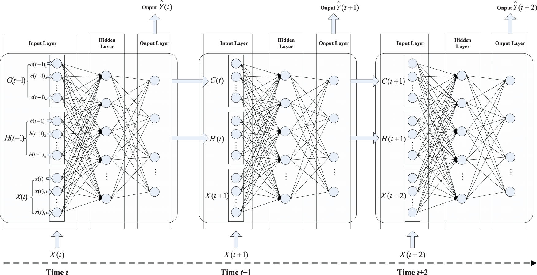
Logical structure diagram of LSTM recurrent neural network.

2.2 Neural unit design and memory realization

The core idea of LSTM is the design of adding unit state c ( t ) and “gate” structure to the hidden layer neural unit. Figure 2 shows the structure of one neural unit in the hidden layer of the network module at time t . The unit state c ( t ) serves as the link of information transmission, allowing the information of each time sequence to be transmitted between network modules at successive moments in the entire network, which is equivalent to long-term memory. Through the state information, the information from the earlier time can be transferred to the later time, which overcomes the influence of short-term memory. Forgetting gates, input gates, and output gates are mainly used for the calculation and processing of data information at the current time and state information at the past time, and are a comprehensive application of short-term memory and long-term memory.

Figure 2

LSTM recurrent neural network hidden layer neural unit structure diagram.

3.1 Algorithm procedure

According to the characteristics of the time series data with equipment spare parts consumption, this article proposes to use LSTM recurrent neural network to predict the requirement of equipment spare parts, in which the technical advantages of LSTM recurrent network will be fully performed. The detailed design of network structure, and the concrete realization of network training and network prediction are shown.

In order to solve the problem that the LSTM recurrent neural network prediction model involves many parameters, which will make the performance of prediction unstable if set artificially, with the goal of minimizing the prediction error, an algorithm of equipment spare part requirement prediction with LSTM recurrent neural network whose parameters are optimized by particle swarm optimization is further proposed. The structural framework of the algorithm is shown in Figure 3.

Figure 3

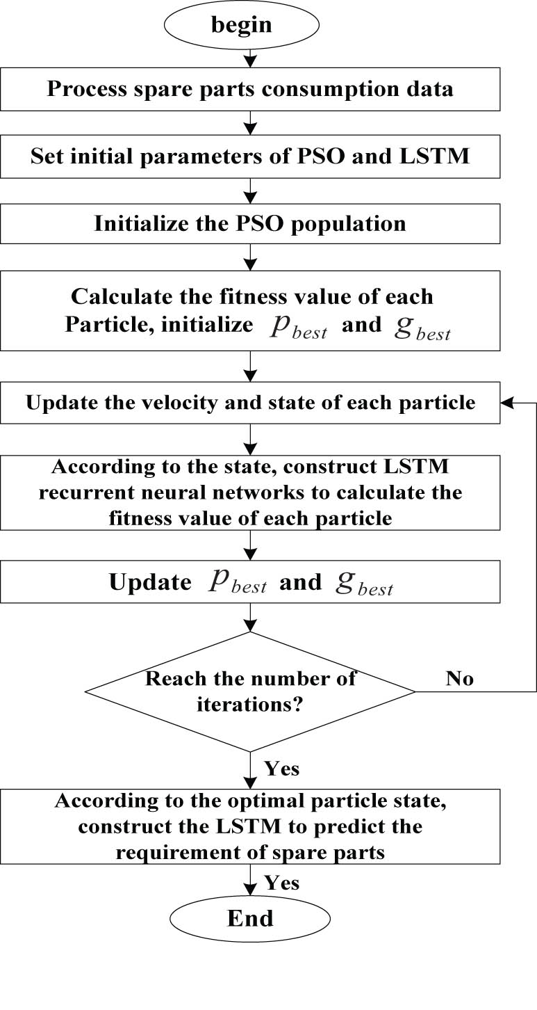
PSO optimizes the LSTM to predict the spare parts requirement.

The specific steps are as follows:

Step 1: Standardize the experimental data and divide it into a training set and a testing set.

Step 2: Set particle swarm algorithm parameter learning factors c 1 and c 2 , maximum inertia weight w max , minimum w min , number of iterations N iter , and number of populations p o p _ s i z e . Setting parameters such as the number of neural units in hidden layer of LSTM recurrent neural network s i z e _ h , prediction interval T , the number of training data subsets MiniBatchSize, and the initial learning rate η as state vectors, initialize the state and velocity of each particle in the population.

Step 3: To each particle, construct an LSTM recurrent neural network according to its four-state vector values, use the training set data to train the network, use the testing set data to test the network, and use the mean square error as the fitness value of each particle.

Step 4: Determine the extreme value p best of the individual and the extreme value g best of the population according to the fitness value of each particle in the population.

Step 5: According to p best and g best , update the state and velocity of each particle in the population.

Step 6: Calculate the fitness value of each particle in the population, and update p best and g best .

Step 7: Repeat steps 4 to 6, and after reaching the number of iterations, use the four-state vectors of particle g best as parameters to construct an LSTM recurrent neural network to predict the requirement of maintenance spare parts.

3.2 Data processing and network construction

The spare parts consumption data is the time series data P = { p 1 , p 2 , ⋯ p t , ⋯ , p n } with monthly intervals, p t represents the consumption of spare parts in tth month. p t = { k 1 t , k 2 t , ⋯ k m t } and k m t represent the consumption quantity of the mth kind of spare parts in t-month. In order to accelerate the convergence of weight parameters when training the network, first use method of z-score to normalize p t . The calculation formula for standardization of time series data is:

The standardized data set P ′ is divided into training set P t r ′ = { p 1 ′ , p 2 ′ , ⋯ , p x ′ } and testing set P t e ′ = { p x + 1 ′ , p x + 2 ′ , ⋯ , p x + y ′ } , x + y = n , x < y .

As the requirement for m kinds of spare parts is predicted based on the consumption data of m kinds of spare parts, the number of neural units in the input layer is m, and the number of neural units in the output layer is also m. The number of hidden layer neural units is s i z e _ h , theoretically the larger the number, the higher the prediction accuracy, but it will increase the amount of network calculations, which can be optimized and determined by the particle swarm algorithm.

3.3 Network training

Set the network training parameters, the number of training cycles MaxEpochs, the number of training data subsets MiniBatchSize, the prediction interval T , and the initial learning rate η . For the training set P t r ′ = { p 1 ′ , p 2 ′ , ⋯ , p x ′ } , take T time data { p 1 ′ , p 2 ′ , ⋯ , p T ′ } initiating from p 1 to calculate the network sequence output { y ˆ ( 1 ) , y ˆ ( 2 ) , ⋯ , y ˆ ( T ) } at time 1 ∼ T through the forward calculation of equations (1)–(7). Then, check { y ˆ ( 1 ) , y ˆ ( 2 ) , ⋯ , y ˆ ( T ) } with { p 2 ′ , p 3 ′ , ⋯ , p T + 1 ′ } at time 2 ∼ T + 1 in the training set. Use the mean square error loss function (13) to calculate the error loss value.

According to the loss function value E t , the reverse transfer algorithm of error data items [22] is used to calculate the adjustment values dU _f , dW _i , dU _i , dW _c , dU _c , dW _o , dU _o , dV, db _f , db _i , db _c , db _o , and db _v of the weights W f , U f , W i , U i , W c , U c , W o , U o , and V and the bias vectors b f , b i , b c , b o , and b v . Continue to take T time data { p 2 ′ , p 3 ′ , ⋯ , p T + 1 ′ } initiating from p 2 to calculate the network timing output value { y ˆ ( 2 ) , y ˆ ( 3 ) , ⋯ , y ˆ ( T + 1 ) } forwardly, then check it with the data { p 3 ′ , p 4 ′ , ⋯ , p T + 2 ′ } at time 3 ∼ T + 2, apply error loss function and reverse transfer algorithm to get the adjustment value of each weight and bias vector, respectively, accumulated with the adjustment value of the previous moment. Follow this method in sequence. After MiniBatchSize times calculation, the weights and bias vectors of the network are updated. The updated value is the cumulative adjustment value multiplied by the learning rate, such as U f = U f + η × d U f , and the adjustment value will return to zero after the update is completed. After MiniBatchSize time data are calculated again, the network weights and bias vectors are updated again. Once the data reaches p x − T + 1 ′ , one training process ends. After repeating MaxEpochs training cycles, the network training is complete. In the training process, the improved Adam optimization algorithm [23] is used to adaptively adjust the learning rate η to make the network training converge as soon as possible, according to the gradient.

3.4 Network prediction

To test the effectiveness of the network, the trained LSTM recurrent neural network and the testing set data P t e ′ = { p x + 1 ′ , p x + 2 ′ , ⋯ , p n ′ } are used to predict data. Starting from p x + 1 ′ , take T time data { p x + 1 ′ , p x + 2 ′ , ⋯ , p x + T ′ } to calculate the output y ˆ ( x + T ) at time x + T according to the equations (1)–(7), continue to take T data from p x + 2 ′ to calculate y ˆ ( x + T + 1 ) until the output y ˆ ( n − 1 ) at time n − 1 is completed. The prediction output set Y = { y ˆ ( x + T ) , y ˆ ( x + T + 1 ) , ⋯ , y ˆ ( n − 1 ) } is de-normalized to obtain the prediction data set P ″ according to equation (13), and the network prediction is completed.

3.5 Parameter optimization

The LSTM recurrent neural network uses the training set data to train the network, optimizes, and adjusts the weight parameters and bias vectors of the input layer, hidden layer, and output layer to obtain a network structure suitable for the prediction object. After the network training is completed, use the testing set data to test the network prediction effect. In the procedure of LSTM recurrent neural network prediction and training, there are four key parameters that affect the quality of the algorithm, which are the number of hidden layer neural units s i z e _ h , the prediction interval T , the number of training data subsets MiniBatchSize, and the initial learning rate η . The influence of these parameters on the algorithm is complicated, and setting by experience is often ineffective. Taking the minimum mean square error of the prediction data set P ″ and the testing set data P t e ′ as the objective function, this article proposes to use the adaptive inertial weight particle swarm algorithm to optimize the four parameters, and use Matlab to implement the algorithm.

4.1 Experimental data and parameter settings

This article takes 48 months consumption data of three main types of maintenance spare parts of a maintenance organization as an example to show the procedure of prediction. The consumption of three types of spare parts is shown in Figure 4.

Figure 4

Consumption of three types of spare parts in a maintenance organization.

The particle swarm algorithm is used to optimize the LSTM recurrent neural network to predict the requirement of equipment maintenance spare parts. The main initial parameter settings of the algorithm are shown in Table 1. Among them, in order to reduce the calculation time, the network training times is set as 100 when using the particle swarm to optimize the LSTM recurrent network parameters, and is set as 300 to enhance the prediction accuracy when using the optimal parameters to construct the network for prediction.

4.2 Simulation result analysis

With the minimum mean square error as the target, the particle swarm algorithm is used to perform 100 iterative calculations, in order to optimize the four key parameters of the LSTM recurrent neural network. The training process is shown in Figure 5. It can be seen that the algorithm converges after 58 iterations, and the optimal mean square error is 3.8524. The four key parameters of the LSTM recurrent neural network are preferably: s i z e _ h = 275, T = 3, MiniBatchSize = 10, and η = 0.3187.

Figure 5

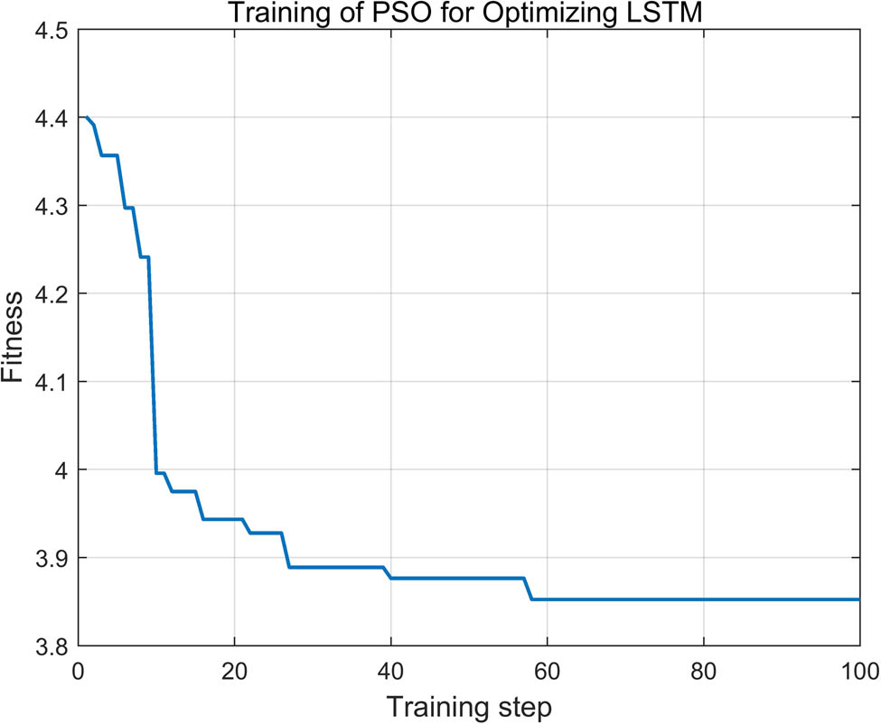
The training process of PSO optimizing the key parameters of LSTM.

The LSTM recurrent neural network is constructed using the four optimal parameters, and the network is trained 1,000 times with 36 months consumption data of three types of spare parts. The values of the loss function in the training process are shown in Figure 6.

Figure 6

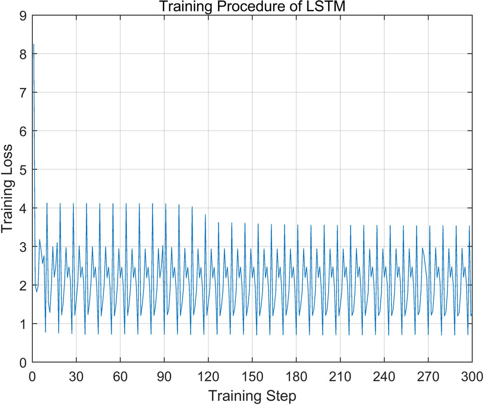
Loss function values in LSTM recurrent neural network training.

Figure 7

Legend of Figures 8–11.

It can be seen that the convergence of the algorithm is good, and the loss function value is low. Using 12 months consumption data to test the trained network, the comparison between the predicted value and the actual consumption value is shown in Figure 8, and the mean square error is 3.3611. The error of the spare parts prediction in August is relatively large because the equipment was suddenly used in large quantities during that period, which was inconsistent with the previous two years.

Figure 8

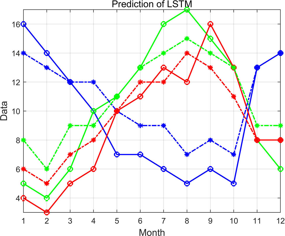
Comparison of LSTM.

Figure 9

Comparison of BP neural network.

Figure 10

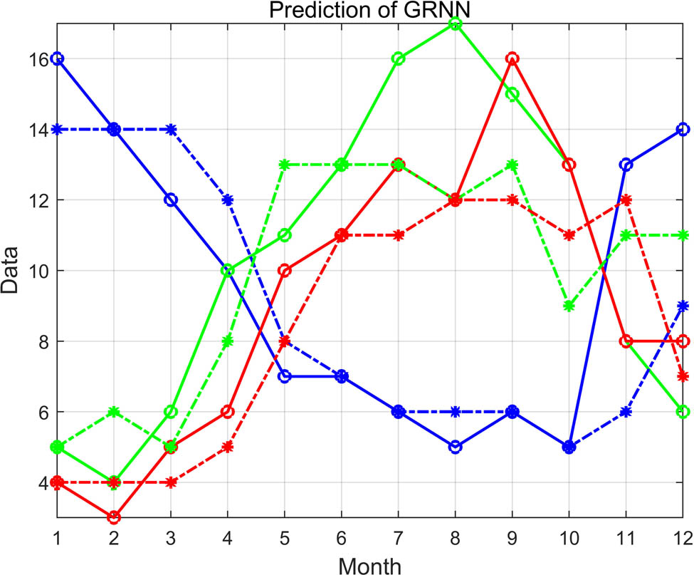
Comparison of GRNN.

Figure 11

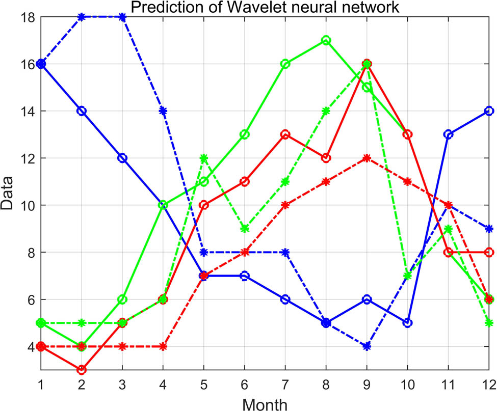
Comparison of wavelet neural network.

In order to verify the predominant prediction performance of the LSTM recurrent neural network, comparative experiments are performed. Four widely used neural networks currently, BP neural network, generalized regression (GRNN) neural network, wavelet neural network, and squeeze-and-excitation networks (SENet) are used to predict the requirement of spare parts too, using the same training set and testing set. After 1,000 times of network training, 12 months requirement for 3 types of maintenance spare parts was predicted, and the comparison between the 3 kinds of neural network prediction values and actual consumption values were obtained, as shown in Figures 9–12. The mean square errors of the four neural networks are shown in Table 2. From the comparison of the predicted value and the actual consumption value curve and the mean square error value, it can be seen that the LSTM recurrent neural network has the highest prediction accuracy and has obvious advantages in predicting the requirement of maintenance spare parts with time series characteristics.

Figure 12

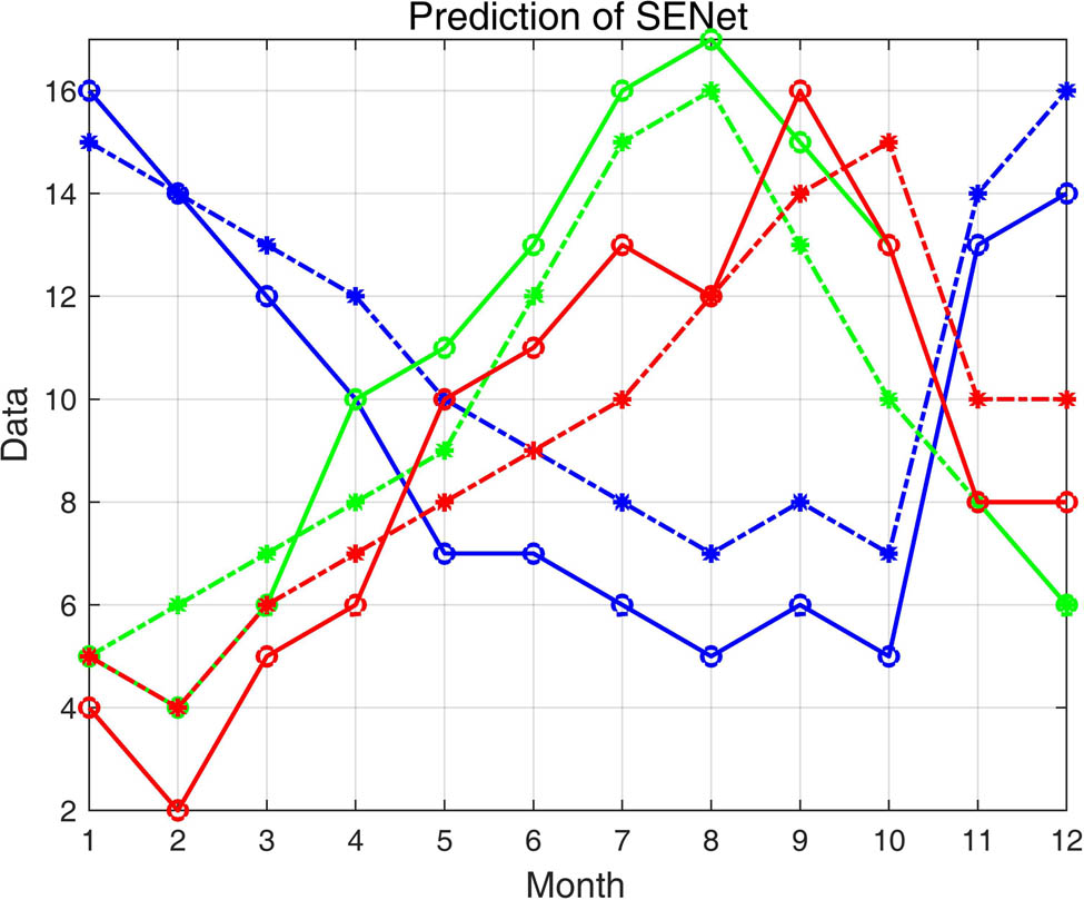
Comparison of SENet.

References

[1] Liu X, Zhu L, Zhang W. Demand forecasting of fuzzy inference-based wartime spares. Acta Armamentarii. 2013;34(9):1197–200.Search in Google Scholar
[2] Wang Y, Ran H, Ren W. A computing method of weibull distribution spare parts demand based on age replacement policy. Fire Control Comm Control. 2017;42(3):64–6.Search in Google Scholar
[3] Kovacs K, Ansari F, Sihn W. A modified Weibull model for service life prediction and spare parts forecast in heat treatment industry. Proc Manuf. 2021;54(7):172–7.10.1016/j.promfg.2021.07.026Search in Google Scholar
[4] Lin C, Feng G, Zishuo W. An optimal combination prediction method of turnover spare parts consumption based on certain weight. J Phys Conf Ser. 2021;1955(1):1–8.10.1088/1742-6596/1955/1/012122Search in Google Scholar
[5] Zhang JX, Si XS, Du DB, Hu CH, Hu C. A novel iterative approach of lifetime estimation for standby systems with deteriorating spare parts. Reliab Eng Syst Saf. 2020;201:1–13.10.1016/j.ress.2020.106960Search in Google Scholar
[6] Chen FL, Chen YC, Kuo JY. Applying moving back-propagation neural network and moving fuzzy neuron network to predict the requirement of critical spare parts. Expert Syst Appl. 2010;37(6):6695–704.10.1016/j.eswa.2010.04.037Search in Google Scholar
[7] Xu S, Zhang H, Nie T, Wang H. Forecasting for materials with intermittent demand based on combined forecasting. Syst Eng Electron. 2012;34(1):111–4.Search in Google Scholar
[8] Yu L, Yang ZB, Tang L. Prediction-based multi-objective optimization for oil purchasing and distribution with the NSGA-II algorithm. Int J Inf Technol Decis Mak. 2016;15(2):423–51.10.1142/S0219622016500097Search in Google Scholar
[9] Mei G, Zhong B, Zhang X, Zhao Z. Combination forecasting model of equipment spare parts demand based on IOWA operator. Ordnance Ind Autom. 2013;32(1):8–11.Search in Google Scholar
[10] Yu F, Li C, Zhang W. Research on the optimal order time of repairable spare parts of aviation. Mater Mech Eng Autom. 2016;198(5):28–30.10.3901/JME.2016.15.028Search in Google Scholar
[11] Liu W, Zhang Y, Dang L. A new prediction model of equipment stock based on gray-Bayesian. Ordnance Ind Autom. 2010;29(4):48–51.Search in Google Scholar
[12] Dou Y, Wang S. Research on spare part requirement prediction of field drill based on BP NN. Ordnance Ind Autom. 2010;29(3):33–4+37.Search in Google Scholar
[13] Luo Y, Xu K. Demand forecast of equipment spare parts based on generalized regression neural network. Precise Manuf Autom. 2014;2:37–8+46.Search in Google Scholar
[14] Guan Z, Chang W. Prediction method of aviation spare parts based on PCA-RBF neural network model. J Beijing Technol Bus Univ (Nat Sci Ed). 2009;27(3):60–4.Search in Google Scholar
[15] Lu Q, Bai M, Peng Y, Zhang W. Armored equipment requirement forecasting based on grey neural network. J Acad Armored Force Eng. 2011;25(6):19–22.Search in Google Scholar
[16] Liu G, Zhong X, Dong X. Research on warship electronic equipments spare parts optimize model based on genetic algorithm and neural network. Ship Sci Technol. 2008;30(5):138–42.Search in Google Scholar
[17] Cao Y, Li Y. Forecasting key spare parts of complex equipments by combining fuzzy neural network and particle swarm optimization. Comput Appl Softw. 2014;31(10):167–71+179.Search in Google Scholar
[18] Zhang H, Nguyen H, Bui XN, Nguyen-Thoi T, Bui TT, Nguyen N, et al. Developing a novel artificial intelligence model to estimate the capital cost of mining projects using deep neural network-based ant colony optimization algorithm. Resour Policy. 2020;66:1–16.10.1016/j.resourpol.2020.101604Search in Google Scholar
[19] Sepp H, Jürgen S. Long short-term memory. Neural Comput. 1997;9(8):1735–80.10.1162/neco.1997.9.8.1735Search in Google Scholar PubMed
[20] Jafarian A, Measoomy Nia S, Khalili Golmankhaneh A, Baleanu D. On artificial neural networks approach with new cost functions. Appl Math Comput. 2018;339:546–55.10.1016/j.amc.2018.07.053Search in Google Scholar
[21] Kim YG, Park ES, Kim BC, Lee SH, Lee SH. Prediction of the major factors for the analysis of the erosion effect on atomic oxygen in LEO satellite using a machine learning method (LSTM). J Aerosp Syst Eng. 2020;14(2):50–6.Search in Google Scholar
[22] Wang X, Wu J, Liu C, Yang H, Du Yanli NI. Exploring LSTM-based recurrent neural network for failures time series prediction. J Beijing Univ Aeronaut Astronaut. 2018;44(4):772–84.Search in Google Scholar
[23] Upadhyay C. Construction of adaptive pulse coupled neural network for abnormality detection in medical images. Appl Artif Intell. 2018;32(6):477–95.10.1080/08839514.2018.1481818Search in Google Scholar
© 2021 Weixing Song et al., published by De Gruyter
This work is licensed under the Creative Commons Attribution 4.0 International License.
Articles in the same Issue
- Regular Articles
- Circular Rydberg states of helium atoms or helium-like ions in a high-frequency laser field
- Closed-form solutions and conservation laws of a generalized Hirota–Satsuma coupled KdV system of fluid mechanics
- W-Chirped optical solitons and modulation instability analysis of Chen–Lee–Liu equation in optical monomode fibres
- The problem of a hydrogen atom in a cavity: Oscillator representation solution versus analytic solution
- An analytical model for the Maxwell radiation field in an axially symmetric galaxy
- Utilization of updated version of heat flux model for the radiative flow of a non-Newtonian material under Joule heating: OHAM application
- Verification of the accommodative responses in viewing an on-axis analog reflection hologram
- Irreversibility as thermodynamic time
- A self-adaptive prescription dose optimization algorithm for radiotherapy
- Algebraic computational methods for solving three nonlinear vital models fractional in mathematical physics
- The diffusion mechanism of the application of intelligent manufacturing in SMEs model based on cellular automata
- Numerical analysis of free convection from a spinning cone with variable wall temperature and pressure work effect using MD-BSQLM
- Numerical simulation of hydrodynamic oscillation of side-by-side double-floating-system with a narrow gap in waves
- Closed-form solutions for the Schrödinger wave equation with non-solvable potentials: A perturbation approach
- Study of dynamic pressure on the packer for deep-water perforation
- Ultrafast dephasing in hydrogen-bonded pyridine–water mixtures
- Crystallization law of karst water in tunnel drainage system based on DBL theory
- Position-dependent finite symmetric mass harmonic like oscillator: Classical and quantum mechanical study
- Application of Fibonacci heap to fast marching method
- An analytical investigation of the mixed convective Casson fluid flow past a yawed cylinder with heat transfer analysis
- Considering the effect of optical attenuation on photon-enhanced thermionic emission converter of the practical structure
- Fractal calculation method of friction parameters: Surface morphology and load of galvanized sheet
- Charge identification of fragments with the emulsion spectrometer of the FOOT experiment
- Quantization of fractional harmonic oscillator using creation and annihilation operators
- Scaling law for velocity of domino toppling motion in curved paths
- Frequency synchronization detection method based on adaptive frequency standard tracking
- Application of common reflection surface (CRS) to velocity variation with azimuth (VVAz) inversion of the relatively narrow azimuth 3D seismic land data
- Study on the adaptability of binary flooding in a certain oil field
- CompVision: An open-source five-compartmental software for biokinetic simulations
- An electrically switchable wideband metamaterial absorber based on graphene at P band
- Effect of annealing temperature on the interface state density of n-ZnO nanorod/p-Si heterojunction diodes
- A facile fabrication of superhydrophobic and superoleophilic adsorption material 5A zeolite for oil–water separation with potential use in floating oil
- Shannon entropy for Feinberg–Horodecki equation and thermal properties of improved Wei potential model
- Hopf bifurcation analysis for liquid-filled Gyrostat chaotic system and design of a novel technique to control slosh in spacecrafts
- Optical properties of two-dimensional two-electron quantum dot in parabolic confinement
- Optical solitons via the collective variable method for the classical and perturbed Chen–Lee–Liu equations
- Stratified heat transfer of magneto-tangent hyperbolic bio-nanofluid flow with gyrotactic microorganisms: Keller-Box solution technique
- Analysis of the structure and properties of triangular composite light-screen targets
- Magnetic charged particles of optical spherical antiferromagnetic model with fractional system
- Study on acoustic radiation response characteristics of sound barriers
- The tribological properties of single-layer hybrid PTFE/Nomex fabric/phenolic resin composites underwater