Revisiting the Reynolds-averaged Navier–Stokes equations

Bohua Sun

doi:10.1515/phys-2021-0102

Article Open Access

Revisiting the Reynolds-averaged Navier–Stokes equations

Bohua Sun

Published/Copyright: January 3, 2022

Published by

Become an author with De Gruyter Brill

Submit Manuscript Author Information Explore this Subject

From the journal Open Physics Volume 19 Issue 1

Abstract

This study revisits the Reynolds-averaged Navier–Stokes (RANS) equations and finds that the existing literature is erroneous regarding the primary unknowns and the number of independent unknowns in the RANS. The literature claims that the Reynolds stress tensor has six independent unknowns, but in fact the six unknowns can be reduced to three that are functions of the three velocity fluctuation components, because the Reynolds stress tensor is simply an integration of a second-order dyadic tensor of flow velocity fluctuations rather than a general symmetric tensor. This difficult situation is resolved by returning to the time of Reynolds in 1895 and revisiting Reynolds’ averaging formulation of turbulence. The study of turbulence modeling could focus on the velocity fluctuations instead of the Reynolds stress. An advantage of modeling the velocity fluctuations is, from both physical and experimental perspectives, that the velocity fluctuation components are observable whereas the Reynolds stress tensor is not.

Keywords: turbulence; number of independent unknowns; Reynolds stress tensor; RANS

1 Introduction

Turbulence is one of the greatest unsolved mysteries of physics (as depicted in Figure 1). After more than a century of studying turbulence, only a few answers have been found regarding how it works and affects the world around us. Many scientists argue that future progress must rely on statistics and increased computing power: extremely fast computer simulations of turbulent flows may help to identify patterns that lead to a theory that organizes and unifies predictions for different situations. Other scientists argue that the phenomenon is so complex that such a fully fledged theory is impossible.

Figure 1

Turbulent smoke. Photograph by B. H. Sun.

Although different researchers might have different views about turbulence, there is consensus that the deterministic Navier–Stokes equations probably contain all the physics information about turbulence. Turbulence can be predicted by understanding and solving the Navier–Stokes equations. Navier [1] and Poisson [2] first introduced these equations, which were finally verified by de Saint-Venant [3] and Stokes [4] based on various considerations regarding the mutual action of the basic fluid molecules [5,6].

This article adopts Reynolds’ deterministic view of turbulence [5] and revisits the Reynolds-averaged Navier–Stokes (RANS) equations. This study addresses a basic problem in turbulence analysis, namely, the number of unknowns in the Reynolds stress tensor, which is obviously also a fundamental question in fluid mechanics. The research herein reveals that the Reynolds stress tensor has only three independent unknowns instead of the six stated in the existing literature, including textbooks. Although the RANS equations were formulated more than 120 years ago, much of the existing literature and standard turbulence textbooks are incorrect regarding the number of unknowns in the RANS, and this has prevented the turbulence problem from being solved. If the number of unknowns is incorrect, then no correct solutions can be possibly obtained, this situation should be corrected to let the turbulence studies not to be compromised.

Given that turbulence is yet to be defined in essence, it would be fitting to return to the beginning of turbulence research, namely, 1895, and consider Reynolds’ seminal studies to rediscover certain useful information. The aims herein are to revisit Reynolds’ averaging formulation of turbulence and clarify the number of independent unknowns in the Reynolds stress tensor and/or RANS equations.

This article is organized as follows. Following an introduction, we introduce Reynolds velocity decomposition and reformulate the RANS equations in tensorial form. We raise an important question about the number of independent unknowns in both the Reynolds stress tensor and RANS equations, and provide three mathematical lemmas and evidence about dyadic tensor. The critical Reynolds number of turbulence transition and other related formulations are derived as well. To demonstrate the Reynolds’ modeling, we quote some results from Reynolds’ paper [5]. Finally, we conclude with perspectives on future developments in turbulence research.

2 Reynolds turbulence equations and RANS equations

The study of the Navier–Stokes equations of incompressible flow is one of the central topics for both laminar and turbulent flows and can be expressed as follows:

(1) ρ ∂ u ∂ t + u ⋅ ( ∇ u ) = − ∇ p + μ ∇ 2 u ,

(2) ∇ ⋅ u = 0 .

Equation (1) is the momentum equation and equation (2) is the mass conservation equation, in which u ( x , t ) is the flow velocity field, x is the vector of spatial coordinates and t is the time, ρ is constant mass density, p ( x , t ) is the flow pressure, μ is the dynamical viscosity, x = x k e k are the position coordinates, e k is a base vector, u is the flow velocity, ∇ = e k ∂ ∂ x k is a gradient operator, and ∇ 2 ( : ) = ∇ ⋅ ∇ ( : ) .

Applying the divergence operation to both sides of the momentum equation (1) and using the mass conservation lead to a pressure equation:

(3) ∇ 2 ⋅ ( p 1 ) = − ρ ∇ ⋅ ( u ⋅ ∇ u ) ,

where 1 = e k e k is an identity tensor.

Infinitesimal analysis reveals that the Navier–Stokes equations admit ten Lie groups, but none is suitable for solving the problem of turbulence. In ground-breaking research, Reynolds [5] considered turbulence from a different perspective and assuming that turbulent motion already exists, he sought to establish a criterion for whether the turbulent character will increase, diminish, or remain stationary [6]. From experiments, Reynolds [5] discovered that turbulence solution could be expressed as the sum of the mean and fluctuating parts of the velocity field, a form of solution not found by Lie group analysis [5]. Mathematically speaking, Reynolds’ solution method can be considered as a general approach to solve nonlinear partial differential equations (PDEs) by transforming them into integro-differential equations.

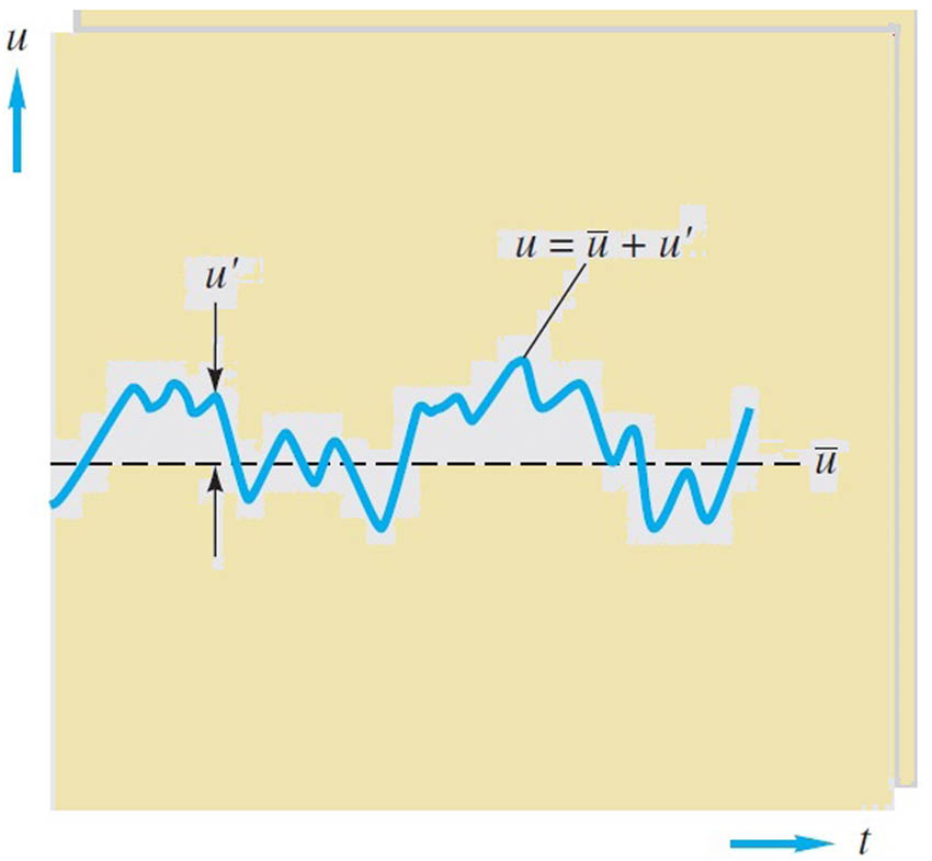
In 1895, Reynolds [5] proposed decomposing the flow velocity u and pressure p into their respective time-averaged quantities u ¯ and p ¯ and their respective fluctuating quantities u ′ and p ′ , as shown in Figures 2 and 3.

Figure 2

Velocity decomposition.

Figure 3

Pressure decomposition.

As such, the Reynolds decompositions are

(4) u ( x , t ) = u ¯ ( x ) + u ′ ( x , t ) ,

(5) p ( x , t ) = p ¯ ( x ) + p ′ ( x , t ) .

Reynolds decomposition converts the four independent unknowns, u and p , into the eight independent unknowns, u ¯ , p ¯ , u ′ , and p ′ .

According to Reynolds [5], u ¯ represents the mean motion at each point and u ′ as a relative motion at the same point; e.g., the time-averaged velocity and pressure are defined as integration transformation as follows:

(6) u ¯ ( x ) = lim T → ∞ 1 T ∫ t t + T u ( x , t ) d t ,

(7) p ¯ ( x ) = lim T → ∞ 1 T ∫ t t + T p ( x , t ) d t ,

or simply [6]

(8) u ¯ ( x ) = 1 T ∫ t t + T u ( x , t ) d t ,

(9) p ¯ ( x ) = 1 T ∫ t t + T p ( x , t ) d t ,

where T is the time period over which the averaging takes place and must be sufficiently large to give meaningful averages to measure mean values. Naturally, the time-fluctuating velocity is u ′ = u − u ¯ ( x ) and the time-fluctuating pressure is p ′ = p − p ¯ ( x ) , both with vanishing time averages, namely, u ¯ ′ = 0 and p ¯ ′ = 0 , respectively.

Reynolds decomposition transforms the Navier-Stokes equations into equations for the mean velocity u ¯ and mean pressure p ¯ as follows:

(10) ρ ∇ ⋅ ( u ¯ ⊗ u ¯ ) + ∇ p ¯ = μ ∇ 2 u ¯ + ∇ ⋅ τ ,

(11) ∇ ⋅ u ¯ = 0 ,

where ⊗ is the tensor product. Hence, the Reynolds stress tensor is defined by

(12) τ ( x ) = − ρ u ′ ⊗ u ′ ¯ = − ρ 1 T ∫ t t + T ( u ′ ⊗ u ′ ) d t ,

which shows that the Reynolds stress depends on the fluctuating velocity field u ′ .

The definition of the Reynolds stress tensor can be written in component form as follows:

(13) τ ( x ) = − ρ u ′ ⊗ u ′ ¯ = − ρ u i ′ u j ′ e i ⊗ e j ¯ = − ρ u i ′ u j ′ ¯ e i ⊗ e j = − ρ 1 T ∫ t t + T ( u i ′ u j ′ ) d t e i ⊗ e j = − ρ 1 T ∫ t t + T ( u 1 ′ u 1 ′ e 1 ⊗ e 1 + u 1 ′ u 2 ′ e 1 ⊗ e 2 + u 1 ′ u 3 ′ e 1 ⊗ e 3 + u 2 ′ u 1 ′ e 2 ⊗ e 1 + u 2 ′ u 2 ′ e 2 ⊗ e 2 + u 2 ′ u 3 ′ e 2 ⊗ e 3 + u 3 ′ u 1 ′ e 3 ⊗ e 1 + u 3 ′ u 2 ′ e 3 ⊗ e 2 + u 3 ′ u 3 ′ e 3 ⊗ e 3 ) d t .

This expression provides a clear information that the three velocity fluctuations u 1 ′ , u 2 ′ , u 3 ′ are the primary unknowns and their time averaging of multiplication of each other produces the Reynolds stress tensor.

To obtain more information about the Reynolds stress tensor, Reynolds [5] derived velocity-fluctuation equations, namely, equation (16) in ref. [5], which he referred to as the equations of momentum of the relative mean motion at each point. The velocity-fluctuation equations in boldface tensorial form are

(14) ρ u , t ′ + ρ ∇ ⋅ ( u ¯ ⊗ u ′ + u ′ ⊗ u ¯ + u ′ ⊗ u ′ ) + ∇ p ′ = μ ∇ 2 u ′ − ∇ ⋅ τ ,

(15) ∇ ⋅ u ′ = 0 .

These are integro-differential equations governing u ¯ , u ′ , and p ′ .

From equation (3) and p = p ¯ + p ′ , by Reynolds averaging, we obtain the mean and fluctuation of pressure equations as follows:

(16) ∇ 2 ⋅ ( p ¯ 1 ) = − ρ ∇ ⋅ ( u ¯ ⋅ ∇ u ¯ + u ′ ⋅ ∇ u ′ ¯ ) , ∇ 2 ⋅ ( p ′ 1 ) = − ρ ∇ ⋅ ( u ¯ ⋅ ∇ u ′ + u ′ ⋅ ∇ u ¯ + u ′ ⋅ ∇ u ′ − u ′ ⋅ ∇ u ′ ¯ )

and

(17) u ′ ⋅ ∇ u ′ ¯ = 1 T ∫ t t + T u ′ ⋅ ∇ u ′ d t = ∇ ⋅ τ .

Denoting the kinematic viscosity as ν = μ / ρ , equations (10) and (11) can be written equivalently in conventional form as

(18) u ¯ ⋅ ∇ u ¯ + 1 T ∫ t t + T ( u ′ ⋅ ∇ u ′ ) d t = − 1 ρ ∇ p ¯ + ν ∇ 2 u ¯ ,

(19) ∇ ⋅ u ¯ = 0 .

The integro-differential equations in equations (10), (11), (14), and (15) are known as the RANS equations formulated by Reynolds [5], who referred to them as the equations of mean motion and relative-to-mean equations at every point. Clearly, the RANS equations are deterministic, not statistical [5,6].

Although the Navier–Stokes equations have been transformed into averaged equations (RANS), such as equations (10), (11), (14), and (15), how to determine their eight unknowns, namely u ¯ , u ′ , p ¯ , and p ′ , is still a challenge. The existing literature only deal with equations (10) and (11) but ignore equations (14) and (15). This ignoring created an issue of determining the Reynolds stress tensor τ .

The literature considers τ as a symmetric tensor with six independent components and it is tempting to model it without using its definition defined in equation (12). In other words, all current modeling on the Reynolds stress tensor τ has been done without using velocity fluctuation u ′ and its intrinsic constraints u ′ ¯ = 0 .

Note that for the deterministic velocity field u ( x , t ) the Reynolds decompositions in equations (4) and (5) are always well defined from equations (8) and (9). In other words, Reynolds decompositions can always be constructed for any flow motion, therefore, Reynolds decomposition might be used as a general method to find a solution for nonlinear PDEs.

3 Number of independent unknowns in Reynolds stress tensor and RANS equations

The existing literature, including textbooks, reports that the Reynolds stress τ has six independent unknowns, namely, τ 11 , τ 12 , τ 13 , τ 22 , τ 23 , and τ 33 . This traditional understanding has resulted in the consensus that there are ten independent unknowns as shown in equations (10) and (11) and/or equations (18) and (19).

In his 1895 paper [5], Reynolds did not discuss the number of independent unknowns in the RANS equations. However, from the flow of his presentation we noted that he never considered the term ρ u ′ ⊗ u ′ ¯ as an independent unknown, while for some cases he proposed explicit expressions for the velocity fluctuation u ′ on page 149 and equation (53) on page 158 of his paper [5]. For instance, on page 149 of ref. [5] he proposed the expression

∑ A r cos r n t + 2 π a x .

Due to limited source of references, the present author is unaware who was the first person to propose the ten unknown perception in equations (10) and (11) of the RANS equations. However, this mistake in classical physics has hampered the development of turbulence as a subject. The RANS equations in equations (10) and (11) comprise four independent equations that govern the mean velocity field, namely, the three components of the Reynolds equation (equation (10)) together with the mean continuity equation (equation (11)).

We show later that the Reynolds stress tensor τ has only three independent unknowns, which are fully determined by the velocity fluctuation components u i ′ ( i = 1 , 2 , 3 ) , because the Reynolds stress tensor is simply an integration of a second-order dyadic tensor of flow velocity fluctuations rather than a general symmetric tensor.

4 Lemmas

The following lemmas support the above statement.

Lemma 4.1

Given two vectors v ( x , t ) = v i e i = v 1 e 1 + v 2 e 2 + v 3 e 3 and w ( x , t ) = w j e j = w 1 e 1 + w 2 e 2 + w 3 e 3 , we can define a dyadic tensor u ⊗ w as follows:

(20) v ⊗ w = v i e i ⊗ w j e j = v i w j e i ⊗ e j = v 1 w 1 e 1 ⊗ e 1 + v 1 w 2 e 1 ⊗ e 2 + v 1 w 3 e 1 ⊗ e 3 + v 2 w 1 e 2 ⊗ e 1 + v 2 w 2 e 2 ⊗ e 2 + v 2 w 3 e 2 ⊗ e 3 + v 3 w 1 e 3 ⊗ e 1 + v 3 w 2 e 3 ⊗ e 2 + v 3 w 3 e 3 ⊗ e 3 .

In general, for v ≠ w , the dyadic tensor u ⊗ w is a general tensor with nine components (elements) and has six independent unknowns, namely, v 1 , v 2 , v 3 and w 1 , w 2 , w 3 , because the nine components are fully determined by the six independent unknowns.

For v = w , the tensor v ⊗ w is a second-order tensor with nine components (elements) and has three independent unknowns, namely, v 1 , v 2 , v 3 and/or w 1 , w 2 , w 3 , because the nine components are fully determined by the three independent unknowns.

Lemma 4.2

Given three vectors u ( x , t ) = u i e i = u 1 e 1 + u 2 e 2 + u 3 e 3 , v ( x , t ) = v i e i = v 1 e 1 + v 2 e 2 + v 3 e 3 , and w ( x , t ) = w j e j = w 1 e 1 + w 2 e 2 + w 3 e 3 , we can define a third-order tensor u ⊗ v ⊗ w as follows:

(21) u ⊗ v ⊗ w = u i e k ⊗ v k e i ⊗ w j e j = u k v i w j e k ⊗ e i ⊗ e j .

In general, for u ≠ v ≠ w , the tensor u ⊗ v ⊗ w is a general tensor with 27 components (elements) and has 9 unknowns, namely, u 1 , u 2 , u 3 and v 1 , v 2 , v 3 and w 1 , w 2 , w 3 , because the 27 components are fully determined by the nine unknowns.

For u = v = w , the tensor u ⊗ v ⊗ w is a third-order tensor with 27 components (elements) and has 3 unknowns, namely, u 1 , u 2 , u 3 or v 1 , v 2 , v 3 and/or w 1 , w 2 , w 3 , because the 27 components are fully determined by the 3 unknowns.

Lemma 4.3

Given a vector v ( x , t ) = v i e i = v 1 e 1 + v 2 e 2 + v 3 e 3 , we can define a second-order symmetric dyadic tensor u ⊗ v and its mean value A ( x ) as follows:

(22) A ( x ) = 1 T ∫ t t + T v ⊗ v d t = 1 T ∫ t t + T v i v j e i ⊗ e j d t = 1 T ∫ t t + T [ v 1 v 1 e 1 ⊗ e 1 + v 1 v 2 e 1 ⊗ e 2 + v 1 v 3 e 1 ⊗ e 3 + v 2 v 1 e 2 ⊗ e 1 + v 2 v 2 e 2 ⊗ e 2 + v 2 v 3 e 2 ⊗ e 3 + v 3 v 1 e 3 ⊗ e 1 + v 3 v 2 e 3 ⊗ e 2 + v 3 v 3 e 3 ⊗ e 3 ] d t ,

where v i v j = v j v i .

Although A ( x ) has six independent components, namely, v 1 v 1 , v 1 v 2 , v 1 v 3 , v 2 v 2 , v 2 v 3 , and v 3 v 3 , it is clear that there are only three independent quantities, namely, v 1 , v 2 , and v 3 , in A ( x ) . This is because the quantities v 1 v 1 , v 1 v 2 , v 1 v 3 , v 2 v 2 , v 2 v 3 , and v 3 v 3 are fully determined by v 1 , v 2 , and v 3 .

Lemma 3 actually states that any (time) averaging operation is merely a method of data processing and does not change the number of unknowns within the problem. Clearly, A ( x ) becomes the Reynolds stress tensor τ upon replacing v 1 , v 2 , v 3 by the velocity fluctuation components u i ′ ( i = 1 , 2 , 3 ) , respectively, namely, v 1 = u 1 ′ , v 2 = u 2 ′ , and v 3 = u 3 ′ .

5 Two proofs

The number of independent unknowns in the Reynolds stress tensor and/or RANS equations should not be an issue at all because it can be found simply from Reynolds’ work [5]. However, the long-standing misconception in the turbulence research community has affected perception. For clarity, it is necessary to explain the issue from the following perspectives.

5.1 Direct proof by definition of Reynolds stress tensor

The lemmas show that the Reynolds stress tensor has three independent unknown components. This is proved by defining the Reynolds stress tensor as

(23) τ ( x ) = − ρ u ′ ⊗ u ′ ¯ = − ρ u i ′ e i ⊗ u j ′ e j ¯ = − ρ u i ′ u j ′ ¯ e i ⊗ e j = − ρ 1 T ∫ t t + T ( u i ′ u j ′ e i ⊗ e j ) d t = − ρ 1 T ∫ t t + T u i ′ u j ′ d t e i ⊗ e j = τ i j e i ⊗ e j ,

and the fluctuation-velocity convective terms are

(24) u ′ ⋅ ∇ u ′ ¯ = u i ′ e i ⋅ [ e k ∂ k ⊗ ( u j ′ e j ) ] ¯ = u i ′ u j , k ′ ¯ e i ⋅ ( e k ⊗ e j ) = u i ′ u j , k ′ ¯ ( e i ⋅ e k ) e j = u i ′ u j , k ′ ¯ δ i k e j = u i ′ u j , i ′ ¯ e j = 1 T ∫ t t + T u i ′ u j , i ′ d t e j = τ i j , i e j = ∇ ⋅ τ ,

where the Reynolds stress tensor τ i j in index form is defined as

(25) τ i j = τ j i = − ρ 1 T ∫ t t + T u i ′ u j ′ d t .

The above indicates that any Reynolds stress tensor component τ i j can be calculated from the fluctuation velocity components u 1 ′ , u 2 ′ , and u 3 ′ , which means that τ i j depends on u 1 ′ , u 2 ′ , and u 3 ′ . In other words, u 1 ′ , u 2 ′ , and u 3 ′ are real independent unknowns. This is the main reason for stating that the Reynolds stress tensor τ has three independent unknowns.

The formulation in equation (23) reveals that the Reynolds stress tensor τ = − ρ u ′ ⊗ u ′ ¯ can be calculated fully from three independent components of the fluctuation velocity, namely, u 1 ′ , u 2 ′ , and u 3 ′ . Therefore, the Reynolds stress tensor has only three unknowns rather than six. This means that the averaging technique is merely a mathematical process that provides a mean value but does not change the number of unknowns of the problem.

The misinterpretation in the literature regarding the number of independent unknown components may stem from considering the Reynolds stress tensor as a general second-order symmetric tensor with six independent components. However, the Reynolds stress tensor is not an arbitrary second-order tensor. In fact, its components are made by the binomial product of the fluctuation velocity components, which means that the Reynolds stress tensor is a dyadic tensor of the velocity fluctuation. The unknown components to construct the dyadic tensor are the three components of fluctuation velocity u ′ . Therefore, the Reynolds stress tensor has only three independent unknowns, namely, u 1 ′ , u 2 ′ , and u 3 ′ . For two-dimensional flow, of course, the two-dimensional Reynolds stress tensor has only two independent unknowns, namely, u 1 ′ and u 2 ′ .

5.2 Proof of a particular case

To construct a second-order tensor or matrix with four components, one can use two scalar functions u ′ = 2 U cos ( ω t ) and v ′ = 2 V cos ( ω t + θ ) as independent unknowns as follows: ( u ′ ) 2 , u ′ v ′ , v ′ u ′ , ( v ′ ) 2 . Thus, the respective time averages are 1 T ∫ t t + T ( u ′ u ′ ) d t = U 2 , 1 T ∫ t t + T ( u ′ v ′ ) d t = U V cos θ , 1 T ∫ t t + T ( v ′ u ′ ) d t = U V cos θ , 1 T ∫ t t + T ( v ′ v ′ ) d t = V 2 . Therefore, the Reynolds stress tensor is

(26) τ = − ρ ( U 2 e 1 ⊗ e 1 + U V cos θ e 1 ⊗ e 2 + V U cos θ e 2 ⊗ e 1 + V 2 e 2 ⊗ e 2 ) .

The above process shows that the independent unknowns are u ′ or U and v ′ or V , which culminate in the Reynolds stress tensor τ .

It is proven once again that both the tensor σ and the Reynolds stress tensor τ are functions of only u 1 ′ , u 2 ′ , and u 3 ′ . The differing views of the independent unknowns in the Reynolds stress tensor are summarized in Table 1.

Table 1

Independent unknowns in Reynolds stress tensor

	Existing literature	Present paper
Number	6	3
Unknowns	τ 11 , τ 12 , τ 13 , τ 22 , τ 23 , τ 33	u 1 ′ , u 2 ′ , u 3 ′

Although the RANS equations are not closed, the four RANS equations in equations (10) and (11) contain only seven independent unknowns instead of ten as stated in the existing literature. The differing views of the independent unknowns in the RANS equations are summarized in Table 2.

Table 2

Independent unknowns in RANS equations

	Existing literature	Present paper
Number	10	7
Unknowns	u ¯ 1 , u ¯ 2 , u ¯ 3	u ¯ 1 , u ¯ 2 , u ¯ 3
	p ¯	p ¯
	τ 11 , τ 12 , τ 13 , τ 22 , τ 23 , τ 33	u 1 ′ , u 2 ′ , u 3 ′

6 Reynolds stress tensor transport equation

Right tensor multiplying from equations (14) by u ′ , we have

(27) ρ u t ′ ⊗ u ′ + ∇ p ′ ⊗ u ′ + ρ [ ∇ ⋅ ( u ¯ ⊗ u ′ + u ′ ⊗ u ¯ + u ′ ⊗ u ′ ) ] ⊗ u ′ = μ ( ∇ 2 u ′ ) ⊗ u ′ + ρ [ ∇ ⋅ ( u ′ ⊗ u ′ ¯ ) ] ⊗ u ′ .

Left tensor multiplying from equations (14) by u ′ , we have

(28) ρ u ′ ⊗ u , t ′ + u ′ ⊗ ∇ p ′ + ρ u ′ ⊗ [ ∇ ⋅ ( u ¯ ⊗ u ′ + u ′ ⊗ u ¯ + u ′ ⊗ u ′ ) ] = μ u ′ ⊗ ( ∇ 2 u ′ ) + ρ u ′ ⊗ [ ∇ ⋅ ( u ′ ⊗ u ′ ¯ ) ] .

Noting the identities: ∇ ⋅ ( u ⊗ v ) = ( ∇ ⋅ u ) v + u ⋅ ∇ v and ∇ ( u ⊗ v ) = ( ∇ u ) ⊗ v + u ⊗ ∇ v ; and continuity conditions ∇ ⋅ u ¯ = 0 and ∇ ⋅ u ′ = 0 , by adding equations (27) and (28) and applying Reynolds averaging, results in the following important equation for the Reynolds stress tensor:

(29) ρ ∂ u ′ ⊗ u ′ ¯ ∂ t + ρ ( u ¯ ⋅ ∇ u ′ + u ′ ⋅ ∇ u ¯ ) ⊗ u ′ ¯ + ρ u ′ ⊗ ( u ¯ ⋅ ∇ u ′ + u ′ ⋅ ∇ u ¯ ) ¯ + ρ [ ( u ′ ⋅ ∇ u ′ ) ⊗ u ′ + u ′ ⊗ ( u ′ ⋅ ∇ u ′ ) ] ¯ + ∇ p ′ ⊗ u ′ ¯ + u ′ ⊗ ∇ p ′ ¯ = μ ( ∇ 2 u ′ ) ⊗ u ′ ¯ + μ u ′ ⊗ ( ∇ 2 u ′ ) ¯ + ρ [ ∇ ⋅ ( u ′ ⊗ u ′ ¯ ) ] ⊗ u ′ ¯ ︸ = 0 + ρ u ′ ⊗ [ ∇ ⋅ ( u ′ ⊗ u ′ ¯ ) ] ¯ ︸ = 0 .

After rearranging we have

(30) ρ ∂ u ′ ⊗ u ′ ¯ ∂ t + ρ u ¯ ⋅ ∇ ( u ′ ⊗ u ′ ¯ ) = − ρ ∇ u ¯ ⋅ ( u ′ ⊗ u ′ ¯ ) − ρ ( u ′ ⊗ u ′ ¯ ) ⋅ ∇ u ¯ − ρ [ ( u ′ ⋅ ∇ u ′ ) ⊗ u ′ ¯ + u ′ ⊗ ( u ′ ⋅ ∇ u ′ ) ¯ ] − ( ( ∇ p ′ ) ⊗ u ′ ¯ + u ′ ⊗ ( ∇ p ′ ) ¯ ) + μ ( ∇ 2 u ′ ) ⊗ u ′ ¯ + μ u ′ ⊗ ( ∇ 2 u ′ ) ¯ .

The existing literature claims that equation (30) has 27 independent unknowns. However, the present research leads to a different opinion, having shown that the Reynolds stress equation (equation (30)) has only seven independent unknowns. Accounting for all symmetries, they are listed in Table 3.

Table 3

Independent unknowns in transport equation of Reynolds stress tensor

	Existing literature	Present paper
Number	27	7
Unknowns	u ¯	u ¯ 1 , u ¯ 2 , u ¯ 3
	u ′	p ′
	( u ′ ⋅ ∇ u ′ ) ⊗ u ′ ¯	u 1 ′ , u 2 ′ , u 3 ′
	u ′ ⊗ ( ∇ p ′ ) ¯
	u ′ ⊗ u ′ ¯

The above statement is proven by the following:

(31) ( u ′ ⋅ ∇ u ′ ) ⊗ u ′ ¯ = u k ′ u j , k ′ u m ′ ¯ e j ⊗ e m = 1 T ∫ t t + T u k ′ u j , k ′ u m ′ d t e j ⊗ e m .

Clearly, the mean values of u k ′ u j , k ′ u m ′ ¯ can be calculated from the velocity fluctuations u 1 ′ , u 2 ′ , and u 3 ′ , which means that u 1 ′ , u 2 ′ , and u 3 ′ are unknowns. Similarly, we have

(32) u ′ ⊗ ( ∇ p ′ ) ¯ = u i ′ ∂ p ′ ∂ x j ¯ e i ⊗ e j = 1 T ∫ t t + T u i ′ ∂ p ′ ∂ x j d t e i ⊗ e j ,

and the mean value of u i ′ ∂ p ′ ∂ x j ¯ can be calculated from p ′ and u 1 ′ , u 2 ′ , and u 3 ′ .

The same can be done for fourth and higher orders as in ref. [7] and textbooks. However, regardless of the order, no additional independent unknowns can be created.

7 Turbulent kinetic energy transport equation

The contraction operation for indexes i and j in equation (30) results in the following transport equation for the turbulent kinetic energy k :

(33) ρ ∂ k ∂ t + ρ u ¯ ⋅ ∇ k = μ ∇ 2 k + ρ ( u ′ ⊗ u ′ ) ¯ : ∇ u ¯ − μ ∇ u ′ : ∇ u ′ ¯ − ∇ ⋅ p ′ u ′ ¯ + 1 2 ρ [ ( u ′ ⋅ u ′ ) u ′ ] ¯ ︸ ,

where the kinetic energy k ( x ) = 1 2 τ k k = 1 2 u k ′ u k ′ ¯ = 1 2 u ′ ⋅ u ′ ¯ = 1 T ∫ t t + T u ′ ⋅ u ′ d t . The independent unknowns in the kinetic energy equation (equation (33)) are summarized in Table 4.

Table 4

Independent unknowns in kinetic energy equation

	Existing literature	Present paper
Number	27	7
Unknowns	u ¯	u 1 ′ , u 2 ′ , u 3 ′
	u ′	u ¯ 1 , u ¯ 2 , u ¯ 3
	u ′ ⊗ u ′ ¯	p ′
	∇ u ′ : ∇ u ′ ¯
	p ′ u ′ ¯
	[ ( u ′ ⋅ u ′ ) u ′ ] ¯

The underbrace term on the right gives zero on integration over the whole region V of the flow, since u ¯ = u ′ = 0 on the boundary surfaces of the region ∂ V or at infinity, namely ∫ V ∇ ⋅ p ′ u ′ ¯ + 1 2 ρ [ ( u ′ ⋅ u ′ ) u ′ ] ¯ d 3 x = ∫ ∂ V p ′ u ′ ¯ + 1 2 ρ [ ( u ′ ⋅ u ′ ) u ′ ] ¯ d 2 x = 0 . This gives an integration invariance relation

(34) ∫ V ρ ∂ k ∂ t + ρ u ¯ ⋅ ∇ k − ρ ( u ′ ⊗ u ′ ) ¯ : ∇ u ¯ − μ ∇ 2 k + μ ∇ u ′ : ∇ u ′ ¯ d 3 x = 0 .

8 Critical Reynolds number of turbulence transition

Introducing dimensionless parameters as η = x L , v = u U , v ¯ = u ¯ U , v ′ = u ′ U , where L is the characteristic length and U is the characteristic length.

The relation (34) can be rewritten as

(35) ∫ V ∂ ∂ t 1 2 v ′ ⋅ v ′ ¯ + 1 2 v ¯ ⋅ ∇ ( v ′ ⋅ v ′ ¯ ) − ( v ′ ⊗ v ′ ) ¯ : ∇ v ¯ − 1 2 1 Re ∇ 2 ( v ′ ⋅ v ′ ¯ ) + 1 Re ∇ v ′ : ∇ v ′ ¯ d 3 η = 0 ,

where the Reynolds number Re = ρ L U μ .

The relation (35) is the energy balance of turbulent flow, which reveals that the velocity fluctuation can only be maintained and sustained if the mean velocity can provide enough energy. In other words, the rate of transformation from energy of mean motion must be equal to the rate at which energy of fluctuation motion is converted into heat. Once the flow has the velocity fluctuation, it means that the flow is in the turbulent state.

(36) Re = ∫ V 1 2 ∇ 2 ( v ′ ⋅ v ′ ¯ ) − ∇ v ′ : ∇ v ′ ¯ d 3 η ∫ V 1 2 v ¯ ⋅ ∇ ( v ′ ⋅ v ′ ¯ ) − ( v ′ ⊗ v ′ ) ¯ : ∇ v ¯ + ∂ ∂ t 1 2 v ′ ⋅ v ′ ¯ d 3 η .

Since the term ∂ ∂ t 1 2 v ′ ⋅ v ′ ¯ is negative, the corresponding energy balance relation (35) provides a limit of the Reynolds number ( Re ) cr or the critical Reynolds number of turbulence transition [8,9], if ∂ ∂ t 1 2 v ′ ⋅ v ′ ¯ is neglected, it leads to

(37) ( Re ) cr = ∫ V 1 2 ∇ 2 ( v ′ ⋅ v ′ ¯ ) − ∇ v ′ : ∇ v ′ ¯ d 3 η ∫ V 1 2 v ¯ ⋅ ∇ ( v ′ ⋅ v ′ ¯ ) − ( v ′ ⊗ v ′ ) ¯ : ∇ v ¯ d 3 η .

This limit of the Reynolds number can be viewed as the generalization of Reynolds’ estimation for 2D problems [5] and has not been reported in the literature.

9 Reynolds’ solution of pressure flow of turbulent fluid between two parallel surfaces and Reynolds computation strategy of the RANS

9.1 Reynolds’ solution of pressure flow of turbulent fluid between two parallel surfaces

As an application of the Reynolds’ decomposition strategy, Reynolds computed a turbulent flow between two parallel surfaces. The detailed calculations can be seen in his paper [5]. Herein, we took only some calculations from his paper as supporting materials for our academic statement on the number of unknowns. The purpose of taking some materials from Reynolds’ paper [5] is to show that Reynolds considered the velocity fluctuations as unknowns rather than the Reynolds stress tensor τ . To maintain consistency with Reynolds [5], in this section, we use Reynolds’ partial differential operator, namely, d ∼ ∂ , e.g., d u / d x = ∂ u / ∂ x .

The fluid is of constant density ρ and viscosity and is caused to flow by a uniform variation of pressure d p ¯ d x in direction x between parallel surfaces, given by y = − h , y = h as shown in Figure 4.

$Figure 4 Flow between two infinite parallel surfaces. Boundary conditions: u = v = w = 0 u=v=w=0 when y = ± h y=\pm h .$

Figure 4

Flow between two infinite parallel surfaces. Boundary conditions: u = v = w = 0 when y = ± h .

If the mean motion is steady and v ¯ = 0 , w ¯ = 0 and u ¯ must satisfy the following.

The boundary condition
(38) u ¯ = 0 , y = ± h .
The equation of continuity
(39) d u ¯ d x = 0 , y = ± h .
The first momentum equation becomes
(40) d p d x = μ d 2 u ¯ d y 2 + d 2 u ¯ d z 2 − ρ d d y ( u ′ v ′ ¯ ) + d d z ( u ′ w ′ ¯ ) ,
or putting
u ¯ = U + u ¯ − U and d p / d x = μ d 2 U / d y 2
as in the singular solution, equation (40) becomes
(41) μ d 2 ( u ¯ − U ) d y 2 + d 2 ( u ¯ − U ) d z 2 = ρ d d y ( u ′ v ′ ¯ ) + d d z ( u ′ w ′ ¯ ) ,
where U = 3 2 u max h 2 − y 2 h 2 , ∫ − h h U d y = 2 h u max , and d p / d x = − ( 3 μ ) u max / h 2 .
The integral of equation (41) over the section of which the left term is zero, and the mean value of μ d u ¯ / d y = μ d U / d y when y = ± h .

The components of relative-mean-motion (i.e., fluctuation) must satisfy the periodic conditions, putting 2c for the limit in direction z .

The equation
(42) ∫ 0 a u ′ d x = ∫ 0 a v ′ d x = ∫ 0 a w ′ d x = 0 , ∫ − h h ∫ − c c u ′ d y d z = 0 .
The equation of continuity
d u ′ / d x + d v ′ / d y + d w ′ / d z + 0 .
The boundary conditions with which the continuity gives
(43) u ′ = v ′ = w ′ = 0 , d u ′ / d x = d v ′ / d y = d w ′ / d z = 0 , when y = ± h .
The condition imposed by symmetrical mean motion,
(44) ∫ − c c d u ′ v ′ ¯ d y + d u ′ w ′ ¯ d z d z = 2 c f ( y 2 ) .

To satisfy the first three relations of equation (43), the expressions for u ′ , v ′ , w ′ must be continuous periodic functions of x , with a maximum periodic distance a , such as sanctify the conditions of continuity.

On page 158 of ref. [5] in the section entitled Expressions for the components of possible relative-mean-motion, Reynolds proposed

(45) u ′ = ∑ 0 ∞ d α n d y + d γ n d z cos ( n l x ) + d β n d y + d δ n d z sin ( n l x ) , v ′ = ∑ 0 ∞ { n l α n sin ( n l x ) − n l β n cos ( n l x ) } , w ′ = ∑ 0 ∞ { n l γ n sin ( n l x ) − n l δ n cos ( n l x ) } ,

where l = 2 π / a . With the above expression, the condition of continuity, d u ′ / d x + d v ′ / d y + d w ′ / d z = 0 , is satisfied.

If the velocity fluctuation is restricted to motion parallel to the plane of x y , γ = δ = w ′ = 0 . Reynolds obtained

(46) u ′ v ′ ¯ = 1 2 ∑ 0 ∞ n l α n d β n d y − β n d α n d y .

Reynolds also compiled integrations by using the above expressions, e.g., equation (58) on page 159 of ref. [5], which is shown as follows:

∬ ρ u ′ v ′ ¯ d u ¯ d y d y d z = 1 2 ∬ ∑ n l α n d β n d y − β n d α n d y d u ¯ d y d y d z .

By giving the above expressions, Reynolds was regarding the velocity fluctuations in u ′ as not only independent unknowns but also deterministic quantities (not random ones).

Reynolds obtained the Reynolds number Re as shown in Figure 5.

(47) Re = ρ ( 2 h ) u max μ = 2 3 14.933 L 4 + 165.412 L 2 + 744.352 L ,

which is minimum if L = 1.621 , hence he predicted the criterion of the Reynolds number of this problem is R cr ≈ 517 (Note: The R cr should be 527.29 after re-calculation).

Figure 5

Reynolds number [5].

9.2 Reynolds computation strategy of the RANS

Regarding the computational aspects of the RANS, we can learn from Reynolds [5]. The way Reynolds dealt with the turbulent flow between two parallel plates clearly shows his idea on the computation of the RANS. Based on Reynolds [5], Reynolds computation methodology can be briefly summarized as follows.

First, solve the corresponding laminar problem of the turbulent problem and use the laminar flow solutions as the mean solutions u ¯ , then cleverly propose velocity fluctuation u ′ that must satisfy both boundary condition and the mass conservation law ∇ ⋅ u ′ = 0 ; in this stage some unknown functions in the u ′ are still needed to be confirmed, then calculate the Reynolds stress tensor τ ( x ) = − ρ u ′ ⊗ u ′ ¯ . Then, we substitute u ¯ , u ′ , and τ in some relevant equations, and to get the following residual vectors, such as Residul 1 = ∇ 2 ⋅ ( p ¯ 1 ) = − ρ ∇ ⋅ ( u ¯ ⋅ ∇ u ¯ + u ′ ⋅ ∇ u ′ ¯ ) , Residul 2 = ∇ 2 ⋅ ( p ′ 1 ) = − ρ ∇ ⋅ ( u ¯ ⋅ ∇ u ′ + u ′ ⋅ ∇ u ¯ + u ′ ⋅ ∇ u ′ − u ′ ⋅ ∇ u ′ ¯ ) . Residul 3 = ρ ∇ ⋅ ( u ¯ ⊗ u ¯ ) + ∇ p ¯ = μ ∇ 2 u ¯ + ∇ ⋅ τ and Residul 4 = ρ u , t ′ + ρ ∇ ⋅ ( u ¯ ⊗ u ′ + u ′ ⊗ u ¯ + u ′ ⊗ u ′ ) + ∇ p ′ = μ ∇ 2 u ′ − ∇ ⋅ τ . Finally, set the four residual vectors equal to zero and to find the unknown functions in the proposed u ′ .

10 Conclusion

This study revisited the RANS equations and studied the primary unknowns and number of independent unknowns in the Reynolds stress tensor and RANS. The present study found that there are three independent unknowns in the Reynolds stress tensor, namely, three velocity fluctuation components u 1 ′ , u 2 ′ , and u 3 ′ . This study not only clarified the number of independent unknowns in the formulations of the RANS equations, but also showed that there are far fewer than traditionally thought.

In the future, the study of turbulence modeling could focus on the velocity fluctuations u 1 ′ , u 2 ′ , and u 3 ′ instead of the Reynolds stress τ i j . An advantage of modeling the velocity fluctuations is that the six unknowns of τ i j are reduced to three u i ′ . In addition, from both physical and experimental perspectives, the velocity fluctuation components are observable, while the Reynolds stress tensors are not.

It is clear that the present ideas and methods might be applicable to the compressible turbulent Navier–Stokes equations, where the mass density ρ and the temperature T must be taken into account, and their Reynolds decompositions ρ = ρ ¯ + ρ ˜ and T = T ¯ + T ˜ should be introduced.

The present investigation can be considered a renaissance of Reynolds’ study in 1895, which will assist with understanding the well-known problem of turbulence that has eluded scientists and mathematicians for more than a century.

Acknowledgements

The author wishes to express his appreciation to the anonymous reviewers for their high-level comments.

Funding information: The author wishes to express his appreciation to the Xi'an University of Architecture and Technology for financial support.
Author contributions: All authors have accepted responsibility for the entire content of this manuscript and approved its submission.
Conflict of interest: The authors state no conflict of interest.
Data availability statement: The data that support the findings of this study are available from the corresponding author upon reasonable request.

References

[1] Navier C. Mémoire sur les Lois du Mouvement des Fluides. Mém.delaAcad.des Sci. 1822;6:389. Search in Google Scholar

[2] Poisson SD . Mémoire sur les Équations géérales de laÉquilibre et du Mouvement des Corps solides élastiques et des fluides. Journ.de laÉcole Plytechn. 1829;13:1. Search in Google Scholar

[3] Saint-Venant AJCB de . Note á joindre au Mémoire sur la dynamique des fluides. Comptes Rendus Acad. sci. Paris. 1943;17:1240–3. Search in Google Scholar

[4] Stokes GG . On the theories of the internal friction of fluids in motion and of the equilibrium and motion of elastic solids. Trans Cambridge Philos Soc. 1845;8:287–319. 10.1017/CBO9780511702242.005Search in Google Scholar

[5] Reynolds O. On the dynamical theory of incompressible viscous fluids and the determination of the criterion. Philosoph Trans R Soc London. 1895;186:123–64. 10.1098/rsta.1895.0004. Search in Google Scholar

[6] Lamb HS . Hydrodynamics. 6th edition. Cambridge: Cambridge University Press; 1993. Search in Google Scholar

[7] Chou P-Y . On velocity correlations and the solutions of the equations of turbulent fluctuation. Q Appl Math. 1945;111(1):38–54. 10.1090/qam/11999Search in Google Scholar

[8] Lee CB , Wu JZ , Transition in wall-bounded flows. Appl Mech Rev. 2008;61(3):030802. 10.1115/1.2909605Search in Google Scholar

[9] Sun BH . Thirty years of turbulence study in China. Appl Math Mech. 2019;40(2):193–214. 10.1007/s10483-019-2427-9Search in Google Scholar

[10] Landau LD , Lifshitz EM . Mechanics. 3rd edition. Oxford: Butterworth-Heinemann; 1976. Search in Google Scholar

Received: 2021-05-06

Revised: 2021-09-27

Accepted: 2021-12-14

Published Online: 2022-01-03

This work is licensed under the Creative Commons Attribution 4.0 International License.

Articles in the same Issue

https://doi.org/10.1515/phys-2021-0102

Keywords for this article

turbulence; number of independent unknowns; Reynolds stress tensor; RANS

Creative Commons

BY 4.0