Position-dependent finite symmetric mass harmonic like oscillator: Classical and quantum mechanical study
-
Biswanath Rath
 ,
Pravanjan Mallick
,
Prachiprava Mohapatra
,
Pravanjan Mallick
,
Prachiprava Mohapatra

Abstract
We formulated the oscillators with position-dependent finite symmetric decreasing and increasing mass. The classical phase portraits of the systems were studied by analytical approach (He’s frequency formalism). We also study the quantum mechanical behaviour of the system and plot the quantum mechanical phase space for necessary comparison with the same obtained classically. The phase portrait in all the cases exhibited closed loop reflecting the stable system but the quantum phase portrait exhibited the inherent signature (cusp or kink) near origin associated with the mass. Although the systems possess periodic motion, the discrete eigenvalues do not possess any similarity with that of the simple harmonic oscillator having m = 1.
1 Introduction
The study of non-linear vibration has become important in designing the flexible structures associated with aircraft, bridge, satellite, etc. [1]. This study can also be extended to acoustics, biology [2], and other branches of engineering such as electronics, robotics, and mechatronics [1]. It is therefore important to design the non-linear control vibration. For the purpose, one needs to consider the simple harmonic oscillator (SHO) with Hamiltonian [3,4]
as a model to design sustained non-linear vibration [2] as long as mass of the system is constant. Further, the closed contour of the phase space of the above system signifies the existence of the discrete energy in the system. At this point, we would like to state that the phase portrait of the operator [5]
is not formed closed orbit and hence it does not possess discrete energy states.
In recent years, systems with position-dependent mass (PDM) have attracted the attention of many researchers and scientists because of their importance in many branches of physics. These systems were first introduced in the theory of semiconductor physics [6,7,8,9,10], especially in the study of the electronic properties and band structure. Subsequently, the applicability of PDM systems can be found in many fields such as quantum mechanics [11,12], classical mechanics [13,14,15], nuclear physics [16], molecular physics [17], neutrino mass oscillations [18], and quantum information [19]. It is worth mentioning here that the PDM study can mostly be related to semiconductors as well as other solid state physics problem. Because of the wide range of applications of PDM, many efforts have been carried out in studying such systems [20,21,22,23,24,25,26,27,28,29,30,31,32,33,34,35,36,37,38,39,40,41,42,43,44,45,46,47,48,49].
It is commonly seen that mass-dependent oscillators having
In this context, we would like to say that at large distance mass becomes zero and the particle possesses infinite kinetic energy and zero potential energy at this point. Therefore, the particle behaves like a free particle and becomes unbound. An unbound particle is most probably unsuitable for any spectral observation. Similarly, considering another form of mass variation as
for which
However, the authors [50] have considered a second model, where mass originates from zero and becomes constant at large distance. The proposed mass model [50] is
A similar type of mass of the form [29,30]
has recently been reported. In a very recent work, another form of decreasing mass
has also been reported [37].
The applicability of increased PDM has also been seen in some experiments. The deuteron–deuteron scattering has successfully explained by considering enhancement of electron mass [51]. The increased effective mass can be used on the basis of fluid to explain some phenomena in quantum field theory [52]. The enhancement of mass of quasiparticle in BaFe2(As1−x P x )2 has been reported at quantum critical point which in turn affect the critical temperature of the superconducting state [53,54]. Effective mass of exciton in semiconductor coupled quantum well is predicted to be enhanced under the influence of electromagnetic field [55]. Enhancement of mass in the quasiparticle led to the entanglement in Kondo problem [56]. In a similar manner, the enhancements of energy of electrons in quasicrystal [57], in hydrogen atom [58], and in quantum LC circuit [59] have also been reported. In addition, the enhancement of mass of electron in periodic lattice using nonlocal approach [60], implication of PDM for semiconductor as well as molecular physics [61], generation of massive photon in a magnetic material [62], etc. have also been predicted recently.
In semiconductors and other problems related to solid state physics, we mainly deal with atoms whose masses cannot be infinite or zero. If it varies with distance, then it must be within the finite values. It is seen that the PDM in all the theoretical cases does not vary within the finite limit. However, in a very recent work, we demonstrated about the finite variation of mass under asymmetric condition [63]. Considering the above literature, we propose a new model position-dependent finite mass variation, i.e.
for symmetric cases comprising of both increasing and decreasing PDM. In view of the importance of vibration and PDM, we focused our attention to study the vibration of a newly designed finite symmetric increasing and decreasing mass harmonic like oscillators using classical and quantum mechanical approaches. The purpose of this work is to choose the PDM that varies between two values avoiding the ambiguity situation as discussed above, i.e., avoiding the values of
The rest of the present work is organized as follows: In Section 2, a classical description of the harmonic like oscillator comprising of both symmetric decreasing and increasing mass is discussed by performing analytical calculations. In Section 3, quantum mechanical study is presented, and finally the discussions along with the important findings of the work are presented in Section 4.
2 Classical description of the system
Consider a particle whose Hamiltonian is given by
The Lagrangian is related to the Hamiltonian as
In our case, we have just one generalized coordinate
Solving equation (10), one can find the Lagrangian (
Using
Substituting equation (12) into the relation
2.1 Decreasing PDM
Let the mass be specified as
Figure 1 shows the variation in
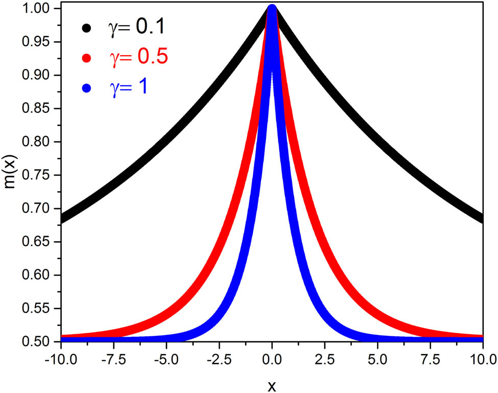
Variation in
Substituting equation (14) in equation (13), we have
The equation (15) can further be simplified to
which leads to
and
This is essentially a modified harmonic oscillator that reflects the amplitude dependence frequency. In other words, vibration of particle is controlled by amplitude or vice versa. Further, it can be regarded as a self-controlled vibration. It is worth mentioning here that one can also be able to derive equation (16b and 16c) following the work of El-Nabulsi and others [64,65,66,67,68,69,70]. When the value of
which is the equation of motion for a free harmonic oscillator.
2.1.1 Analytical calculation on decreasing PDM
Let us rewrite the equation of motion (equation 16(b)) as
where
with
The equation (18) has the similarity with the Kryloff–Bogoliuboff autonomous system, which is expressed as [5]
with the solution is of the form
It should be stated here that
In our analytical approach, we assume a similar type of solution as
in which the frequency of oscillation (
where
and
To obtain the expression of the value of
Figure 2 showed the variation in frequency (

Variation in frequency (

Variation in (a) x with respect to time t, (b)
2.2 Increasing PDM
Here, we consider an increasing position-dependent mass, which is expressed as
Figure 4 shows the variation in

Variation in
2.2.1 Analytical calculation on increasing PDM
Substituting equation (26) in equation (13) and simplifying, we have
In this case, we also consider the formalism discussed above (in Section 2.1.1) to derive the frequency of oscillation for the solution to equations (27a and 27b) using the He’s formalism [63,71,72,73] as
The analytical results on the variation in

Variation in (a)
3 Quantum mechanical study
In this case, we solve the eigenvalue relation using matrix diagonalization method [22,63,74,75,76,77] as
where
Here,
Using the above-mentioned procedure, one can get the recursion relation satisfied by
where
The energy eigenvalues of the Hamiltonian (equation (8)) with PDM (equation (14)) are obtained following the above-mentioned procedure for different values of
for our quantum mechanical calculation following the work of Wilkes and Muljarov [55].
First five eigenvalues of Hamiltonian (equation (8)) with PDM (equation (14)) with different values of
| Energy level (
|
|
Eigenvalue (
|
|---|---|---|
| 0 | 0.1 | 0.5 |
| 1 | 1.4725 | |
| 2 | 2.4458 | |
| 3 | 3.4060 | |
| 4 | 4.3667 | |
| 0 | 0.5 | 0.5 |
| 1 | 1.3846 | |
| 2 | 2.2946 | |
| 3 | 3.1659 | |
| 4 | 4.0635 | |
| 0 | 1 | 0.5 |
| 1 | 1.3281 | |
| 2 | 2.2570 | |
| 3 | 3.1322 | |
| 4 | 4.0761 |
First five eigenvalues of Hamiltonian (equation (8)) with PDM (equation (26)) with different values of
| Energy level (
|
|
Eigenvalue (
|
|---|---|---|
| 0 | 0.1 | 0.5 |
| 1 | 1.536 | |
| 2 | 2.5699 | |
| 3 | 3.6203 | |
| 4 | 4.6675 | |
| 0 | 0.5 | 0.5 |
| 1 | 1.6353 | |
| 2 | 2.7172 | |
| 3 | 3.8568 | |
| 4 | 4.9540 | |
| 0 | 1 | 0.5 |
| 1 | 1.6922 | |
| 2 | 2.7526 | |
| 3 | 3.9041 | |
| 4 | 4.9618 |
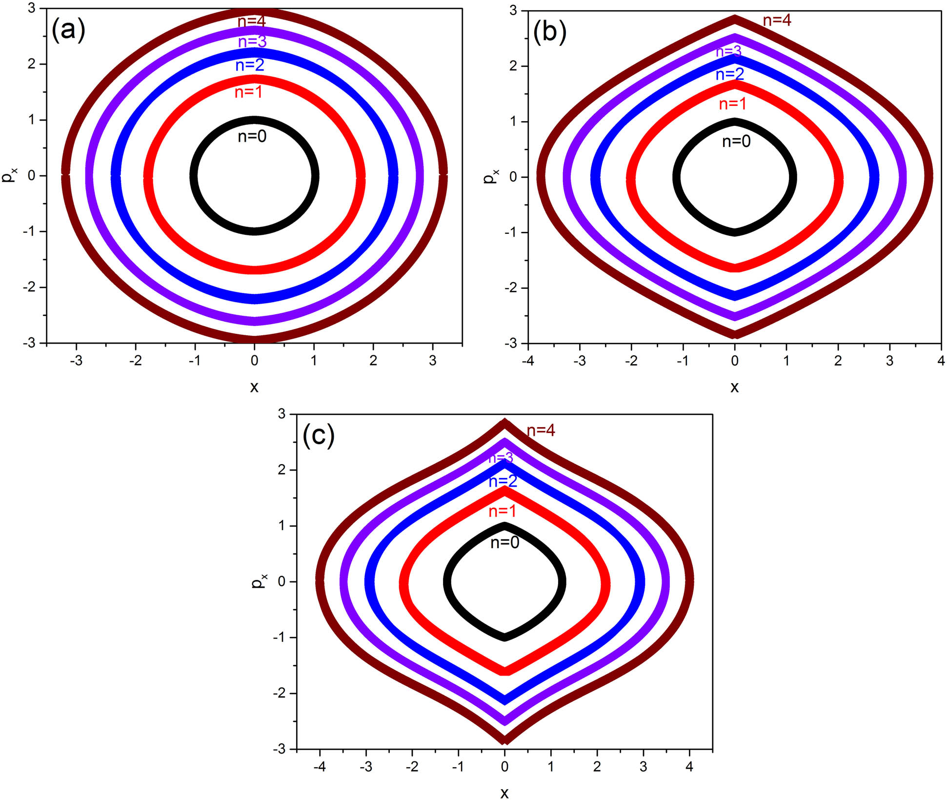
To have more information about the system, we plot quantum mechanical phase trajectories of the system (i) with PDM (equation (14)) with different values of

4 Discussion and conclusion
The Harmonic like oscillator under the influence of decreasing and increasing PDM has been studied. In the case of increasing mass,
In conclusion, the present model analysis can be extended to PDM that varies between any finite values of
Acknowledgments
The authors sincerely thank the reviewer 1 for giving them valuable comments along with some relevant references on mass variation which helped them for the overall improvement of the manuscript. The authors Jihad Asad, Hussein Shanak, and Rabab Jarrar would like to thank Palestine Technical University – Kadoorie.
-
Conflict of interest: Authors state no conflict of interest.
References
[1] David W, Simon N. Nonlinear Vibration with Control for Flexible and Adaptive Structures. Netherlands: Springer; 2010.Search in Google Scholar
[2] Rath B, Agarwalla S. Nonlinear oscillator: controlled and uncontrolled vibrations. Proc Natl Acad Sci, India, Sect A Phys Sci. 2014;84(1):83–66.10.1007/s40010-013-0110-8Search in Google Scholar
[3] Resnick R, Halliday D. Physics, Part-I. New York: John Wiley & Sons. Inc; 1966.Search in Google Scholar
[4] Biswas SN. Classical mechanics. Kolkata: Books and Allied (P) Ltd.; 1998.Search in Google Scholar
[5] Gupta KC. Classical mechanics of particles and rigid body. New Delhi: New Age International (P) Ltd; 1997.Search in Google Scholar
[6] Oldwig von R. Position-dependent effective masses in semiconductor theory. Phys Rev. 1983;B27:7547.10.1103/PhysRevB.27.7547Search in Google Scholar
[7] Ganguly A, Kuru Ş, Negro J, Nieto L. A study of the bound states for square potential wells with position-dependent mass. Phys Lett A. 2006;360:228–33.10.1016/j.physleta.2006.08.032Search in Google Scholar
[8] Silveririnha MG, Engheta N. Transformation electronics: Tailoring the effective mass of electrons. Phys Rev B. 2012;86:161104(R).10.1103/PhysRevB.86.161104Search in Google Scholar
[9] Chen Y, Yan Z, Mihalache D, Malomed BA. Families of stable solitons and excitations in the PT-symmetric nonlinear Schrödinger equations with position-dependent effective masses. Sci Rep. 2017;7:1257.10.1038/s41598-017-01401-3Search in Google Scholar
[10] Morrow RA. Establishment of an effective-mass Hamiltonian for abrupt heterojunctions. Phys Rev B. 1987;35:8074–79; Morrow RA. Effective-mass Hamiltonians for abrupt heterojunctions in three dimensions. Phys Rev B. 1987;36:4836.10.1103/PhysRevB.35.8074Search in Google Scholar
[11] de Saavedra, FA, Boronat J, Polls A, Fabrocini A. Effective mass of one He4 atom in liquid He3. Phys Rev B. 1994;50:4248–51.10.1103/PhysRevB.50.4248Search in Google Scholar
[12] Serra L, Lipparini E. Spin response of unpolarized quantum dots. Europhys Lett. 1997;40:667–72.10.1209/epl/i1997-00520-ySearch in Google Scholar
[13] Lakshmanan M. On a non-linear harmonic oscillator. J Sound Vib. 1979;64:458–61.10.1016/0022-460X(79)90592-3Search in Google Scholar
[14] Carinena JF, Ranada MF, Santander M. One-dimensional model of a quantum nonlinear harmonic oscillator. Rep Math Phys. 2004;54:285–93.10.1016/S0034-4877(04)80020-XSearch in Google Scholar
[15] Flores J, Solovey G, Gil S. Variable mass oscillator. Am J Phys. 2003;71:721–55.10.1119/1.1571838Search in Google Scholar
[16] Bonatsos D, Georgoudis PE, Minkov N, Petrellis D, Quesne C. Bohr Hamiltonian with a deformation-dependent mass term for the Kratzer potential. Phys Rev C. 2013;88:034316.10.1103/PhysRevC.88.034316Search in Google Scholar
[17] Ovando G, Peña JJ, Morales J. Position-dependent mass Schrödinger equation for the Morse potential. J Phys: Conf Ser. 2017;792:012037.10.1088/1742-6596/792/1/012037Search in Google Scholar
[18] Bethe HA. Possible explanation of the solar-neutrino puzzle. Phys Rev Lett. 1986;56:1305–8.10.1201/9780429502811-95Search in Google Scholar
[19] Falaye BJ, Serrano FA, Shi-Hai D. Fisher information for the position-dependent mass Schrödinger system. Phys Lett A. 2016;380:267–71.10.1016/j.physleta.2015.09.029Search in Google Scholar
[20] Baleanu D, Jajarmi A, Sajjadi SS, Asad JH. The fractional features of a harmonic oscillator with position-dependent mass. Commun Theor Phys. 2020;72:055002.10.1088/1572-9494/ab7700Search in Google Scholar
[21] Mustafa O. Position-dependent mass harmonic oscillator: classical-quantum mechanical correspondence and ordering-ambiguity. arXiv:1208.2109v3 [quant-ph].Search in Google Scholar
[22] Rath B, Mallick P, Akande J, Mohapatra PP, Adjaї DKK, Koudahoun LH, et al. Asymmetric variation of a finite mass harmonic like oscillator. Proc Indian Natl Sci Acad. 2017;83:935–40.Search in Google Scholar
[23] Ruby VC, Senthilvelan M. On the construction of coherent states of position dependent mass Schrödinger equation endowed with effective potential. J Math Phys. 2010;51:052106-1–14.10.1063/1.3374667Search in Google Scholar
[24] Chargui Y, Dhahbi A, Trabelsi A. A novel approach for constructing kinetic energy operators with position dependent mass. Results Phys. 2019;13:102329.10.1016/j.rinp.2019.102329Search in Google Scholar
[25] Tiwari AK, Pandey SN, Santhilvelan M, Lakshmanan M. Classification of Lie point symmetries for quadratic Liénard type equation ẍ + f(x)ẋ2 + g(x) = 0. J Math Phys. 2013;54:053506.10.1063/1.4803455Search in Google Scholar
[26] Lakshmanan M, Chandrasekar VK. Generating finite dimensional integrable nonlinear dynamical systems. Eur Phys J ST. 2013;222:665–88.10.1140/epjst/e2013-01871-6Search in Google Scholar
[27] Musielak ZE. Standard and non-standard Lagrangians for dissipative dynamical systems with variable coefficients. J Phys A: Math Theor. 2008;41:055205.10.1088/1751-8113/41/5/055205Search in Google Scholar
[28] Mathews PM, Lakshmanan M. On a unique nonlinear oscillator. Quart Appl Math. 1974;32:215–88.10.1090/qam/430422Search in Google Scholar
[29] Yañez-Navarro G, Guo-Hua S, Dytrych T, Launey KD, Shi-Hai D, Draayer JP. Quantum information entropies for position-dependent mass Schrödinger problem. Ann Phys. 2014;348:153–60.10.1016/j.aop.2014.05.018Search in Google Scholar
[30] Guo-Hua S, Popov D, Camacho-Nieto O, Shi-Hai D. Shannon information entropies for position-dependent mass Schrödinger problem with a hyperbolic well. Chin Phys B. 2015;24:100303.10.1088/1674-1056/24/10/100303Search in Google Scholar
[31] Mustafa O. PDM creation and annihilation operators of the harmonic oscillators and the emergence of an alternative PDM-Hamiltonian. Phys Lett A. 2020;384:126265.10.1016/j.physleta.2020.126265Search in Google Scholar
[32] Biswas K, Saha JP, Patra P. On the position-dependent effective mass Hamiltonian. Eur Phys J Plus. 2020;135:457.10.1140/epjp/s13360-020-00476-8Search in Google Scholar
[33] Bravo R, Plyushchay MS. Position-dependent mass, finite-gap systems, and supersymmetry. Phys Rev D. 2016;93:105023.10.1103/PhysRevD.93.105023Search in Google Scholar
[34] Mustafa O, Algadhi Z. Position-dependent mass momentum operator and minimal coupling: point canonical transformation and isospectrality. Eur Phys J Plus. 2019;134:228.10.1140/epjp/i2019-12588-ySearch in Google Scholar
[35] Quesne C. Deformed shape invariance symmetry and potentials in curved space with two known eigenstates. J Math Phys. 2018;59:042104.10.1063/1.5017809Search in Google Scholar
[36] Zhao FQ, Liang XX, Ban SL. Influence of the spatially dependent effective mass on bound polarons in finite parabolic quantum wells. Eur Phys J B. 2003;33:3–8.10.1140/epjb/e2003-00134-3Search in Google Scholar
[37] El-Nabulsi RA. Inverse-power potentials with positive-bound energy spectrum from fractal, extended uncertainty principle and position-dependent mass arguments. Eur Phys J Plus. 2020;135:693.10.1140/epjp/s13360-020-00717-wSearch in Google Scholar
[38] El-Nabulsi RA. Scalar particle in new type of the extended uncertainty principle. Few Body Syst. 2020;61:1–10.10.1007/s00601-019-1534-8Search in Google Scholar
[39] El-Nabulsi RA. A new approach to the Schrodinger equation with position-dependent mass and its implications in quantum dots and semiconductors. J Phys Chem Solid. 2020;140:109384.10.1016/j.jpcs.2020.109384Search in Google Scholar
[40] El-Nabulsi RA. A generalized self-consistent approach to study position-dependent mass in semiconductors organic heterostructures and crystalline impure materials. Phys E: Low Dim Syst Nanostruct. 2020;124:114295.10.1016/j.physe.2020.114295Search in Google Scholar
[41] El-Nabulsi RA. Dynamics of position-dependent mass particle in crystal lattices microstructures. Phys E: Low Dim Syst Nanostruct. 2020;127:114525.10.1016/j.physe.2020.114525Search in Google Scholar
[42] El-Nabulsi RA. Path integral method for quantum dissipative systems with dynamical friction: applications to quantum dots/zero-dimensional nanocrystals. Superlattices Microstruct. 2020;144:106581.10.1016/j.spmi.2020.106581Search in Google Scholar
[43] El-Nabulsi RA. On a new fractional uncertainty relation and its implications in quantum mechanics and molecular physics. Proc R Soc A. 2020;476:20190729.10.1098/rspa.2019.0729Search in Google Scholar
[44] El-Nabulsi RA. Some implications of three generalized uncertainty principles in statistical mechanics of an ideal gas. Eur Phys J Plus. 2020;135:34.10.1140/epjp/s13360-019-00051-wSearch in Google Scholar
[45] El-Nabulsi RA. Some implications of position-dependent mass quantum fractional Hamiltonian in quantum mechanics. Eur Phys J Plus. 2019;134:192.10.1140/epjp/i2019-12492-6Search in Google Scholar
[46] Von Roos O. Position-dependent effective masses in semiconductor theory. Phys Rev. 1983;B27:7547–52.10.1103/PhysRevB.27.7547Search in Google Scholar
[47] Yu J, Dong SH, Sun GH. Series solutions of the Schrödinger equation with position-dependent mass for the Morse potential. Phys Lett A. 2004;322:290–77.10.1016/j.physleta.2004.01.039Search in Google Scholar
[48] Dong SH, Pena JJ, Pacheco-Garcia C, Garcia-Ravelo J. Vasodilatory mechanism of levobunolol on vascular smooth muscle cells. Mod Phys Lett A. 2007;22:1039–45.10.1016/j.exer.2007.01.010Search in Google Scholar PubMed
[49] Mustafa O, Algadhi Z. Position-dependent mass charged particles in magnetic and Aharonov–Bohm flux fields: separability, exact and conditionally exact solvability. Eur Phys J Plus. 2020;135:559.10.1140/epjp/s13360-020-00529-ySearch in Google Scholar
[50] Negro J, Nieto LM. On position-dependent mass harmonic oscillators. J Phys: Conf Ser. 2008;128:012053.10.1088/1742-6596/128/1/012053Search in Google Scholar
[51] Davidson M. Variable mass theories in relativistic quantum mechanics as an explanation for anomalous low energy nuclear phenomena. J Phys: Conf Ser. 2015;615:012016.10.1088/1742-6596/615/1/012016Search in Google Scholar
[52] Pinto MB. Introducing the notion of bare and effective mass via Newton’s second law of motion. Eur J Phys. 2007;28:171.10.1088/0143-0807/28/2/003Search in Google Scholar
[53] Walmsley P, Putzke C, Malone L, Guillamón I, Vignolles D, Proust C, et al. Quasiparticle mass enhancement close to the quantum critical point in BaFe2(As(1−x)P(x))2. Phys Rev Lett. 2013;110:257002.10.1103/PhysRevLett.110.257002Search in Google Scholar PubMed
[54] Grinenko V, Iida K, Kurth F, Efremov DV, Drechsler SL, Cherniavskii I, et al. Selective mass enhancement close to the quantum critical point in BaFe2(As1−x Px)2. Sci Rep. 2017;7:4589.10.1038/s41598-017-04724-3Search in Google Scholar PubMed PubMed Central
[55] Wilkes J, Muljarov EA. Exciton effective mass enhancement in coupled quantum wells in electric and magnetic fields. N J Phys. 2016;18:023032.10.1088/1367-2630/18/2/023032Search in Google Scholar
[56] Pari NAÁ, García DJ, Cornaglia PS. Quasiparticle mass enhancement as a measure of entanglement in the Kondo problem. Phys Rev Lett. 2020;125:217601.10.1103/PhysRevLett.125.217601Search in Google Scholar PubMed
[57] El-Nabulsi RA. Emergence of quasiperiodic quantum wave functions in Hausdorff dimensional crystals and improved intrinsic carrier concentrations. J Phys Chem Solids. 2019;127:224–30.10.1016/j.jpcs.2018.12.025Search in Google Scholar
[58] El-Nabulsi RA. Nonlocal uncertainty and its implications in quantum mechanics at ultramicroscopic scales. Quant Stud: Math Found. 2019;6:123–33.10.1007/s40509-018-0170-1Search in Google Scholar
[59] El-Nabulsi RA. Modeling of electrical and mesoscopic circuits at quantum nanoscale from heat momentum operator. Phys E: Low Dim Syst Nanostruct. 2018;98:90–104.10.1016/j.physe.2017.12.026Search in Google Scholar
[60] El-Nabulsi RA. Nonlocal approach to energy bands in periodic lattices and emergence of electron mass enhancement. J Phys Chem Solids. 2018;122:167–73.10.1016/j.jpcs.2018.06.028Search in Google Scholar
[61] El-Nabulsi RA. Time-fractional Schrödinger equation from path integral and its implications in quantum dots and semiconductors. Eur Phys J Plus. 2018;133:394.10.1140/epjp/i2018-12254-0Search in Google Scholar
[62] El-Nabulsi RA. Massive photons in magnetic materials from nonlocal quantization. J Magn Magn Mater. 2018;458:213–66.10.1016/j.jmmm.2018.03.012Search in Google Scholar
[63] Asad J, Mallick P, Samei ME, Rath B, Mohapatra P, Shanak H, et al. Asymmetric variation of a finite mass harmonic like oscillator. Results Phys. 2020;19:103335.10.1016/j.rinp.2020.103335Search in Google Scholar
[64] El-Nabulsi RA. A generalized nonlinear oscillator from non-standard degenerate Lagrangians and its consequent Hamiltonian formalism. Proc Natl Acad Sci, India, Sect A Phys Sci. 2014;84:563–99.10.1007/s40010-014-0159-zSearch in Google Scholar
[65] Cariñena JF, Rañada MF, Santander M, Senthilvelan M. A non-linear oscillator with quasi-harmonic behaviour: two- and n-dimensional oscillators. Nonlinearity. 2004;17:1941–63.10.1088/0951-7715/17/5/019Search in Google Scholar
[66] Chandrasekar VK, Senthilvelan M, Lakshmanan M. Unusual Liénard-type nonlinear oscillator. Phys Rev E. 2005;72:066203–11.10.1103/PhysRevE.72.066203Search in Google Scholar PubMed
[67] El-Nabulsi RA. Non-standard Lagrangians with higher-order derivatives and the Hamiltonian formalism. Proc Natl Acad Sci, India, Sect A Phys Sci. 2015;85:247–52.10.1007/s40010-014-0192-ySearch in Google Scholar
[68] El-Nabulsi RA. Fractional oscillators from non-standard Lagrangians and time-dependent fractional exponent. Comp Appl Math. 2014;33:163–79.10.1007/s40314-013-0053-3Search in Google Scholar
[69] El-Nabulsi RA. Non-standard Lagrangians in quantum mechanics and their relationship with attosecond laser pulse formalism. Lasers Eng (Old City Publ). 2018;40(4–6):347–74.Search in Google Scholar
[70] El-Nabulsi RA. Path integral formulation of fractionally perturbed Lagrangian oscillators on fractal. J Stat Phys. 2018;172(6):1617–40.10.1007/s10955-018-2116-8Search in Google Scholar
[71] He JH. Some asymptotic methods for strongly nonlinear equations. Int J Mod Phys B. 2006;20:1141–99.10.1142/S0217979206033796Search in Google Scholar
[72] He JH. An elementary introduction to recently developed asymptotic methods and nanomechanics in textile engineering. Int J Mod Phys B. 2008;22(21):3487–78.10.1142/S0217979208048668Search in Google Scholar
[73] Rath B. Some studies on: ancient Chinese formalism, He's frequency formulation for nonlinear oscillators and “Optimal Zero Work” method. Orissa J Phys. 2011;18(1):109.Search in Google Scholar
[74] Rath B, Mallick P, Samal PK. Real spectra of isospectral non-hermitian hamiltonians. Afr Rev Phys. 2014;9(0027):201–5.Search in Google Scholar
[75] Rath B. Iso-spectral instability of harmonic oscillator: breakdown of unbroken pseudo-hermiticity and PT symmetry condition. Afr Rev Phys. 2015;10(0051):427–34.Search in Google Scholar
[76] Chaudhuri RN, Mondal M. Hill determinant method with a variational parameter. Phys Rev A. 1989;40:6080–3.10.1103/PhysRevA.40.6080Search in Google Scholar PubMed
[77] Banerjee K, Bhatnagar SP, Choudhry V, Kanwal SS. The anharmonic oscillator. Proc R Soc Lond A. 1978;360:575–86.10.1098/rspa.1978.0086Search in Google Scholar
[78] Lanczewski T. Motion of a classical object with oscillating mass. arxiv:1103.3402v1 [physics.gen-ph].Search in Google Scholar
© 2021 Biswanath Rath et al., published by De Gruyter
This work is licensed under the Creative Commons Attribution 4.0 International License.
Articles in the same Issue
- Regular Articles
- Circular Rydberg states of helium atoms or helium-like ions in a high-frequency laser field
- Closed-form solutions and conservation laws of a generalized Hirota–Satsuma coupled KdV system of fluid mechanics
- W-Chirped optical solitons and modulation instability analysis of Chen–Lee–Liu equation in optical monomode fibres
- The problem of a hydrogen atom in a cavity: Oscillator representation solution versus analytic solution
- An analytical model for the Maxwell radiation field in an axially symmetric galaxy
- Utilization of updated version of heat flux model for the radiative flow of a non-Newtonian material under Joule heating: OHAM application
- Verification of the accommodative responses in viewing an on-axis analog reflection hologram
- Irreversibility as thermodynamic time
- A self-adaptive prescription dose optimization algorithm for radiotherapy
- Algebraic computational methods for solving three nonlinear vital models fractional in mathematical physics
- The diffusion mechanism of the application of intelligent manufacturing in SMEs model based on cellular automata
- Numerical analysis of free convection from a spinning cone with variable wall temperature and pressure work effect using MD-BSQLM
- Numerical simulation of hydrodynamic oscillation of side-by-side double-floating-system with a narrow gap in waves
- Closed-form solutions for the Schrödinger wave equation with non-solvable potentials: A perturbation approach
- Study of dynamic pressure on the packer for deep-water perforation
- Ultrafast dephasing in hydrogen-bonded pyridine–water mixtures
- Crystallization law of karst water in tunnel drainage system based on DBL theory
- Position-dependent finite symmetric mass harmonic like oscillator: Classical and quantum mechanical study
- Application of Fibonacci heap to fast marching method
- An analytical investigation of the mixed convective Casson fluid flow past a yawed cylinder with heat transfer analysis
- Considering the effect of optical attenuation on photon-enhanced thermionic emission converter of the practical structure
- Fractal calculation method of friction parameters: Surface morphology and load of galvanized sheet
- Charge identification of fragments with the emulsion spectrometer of the FOOT experiment
- Quantization of fractional harmonic oscillator using creation and annihilation operators
- Scaling law for velocity of domino toppling motion in curved paths
- Frequency synchronization detection method based on adaptive frequency standard tracking
- Application of common reflection surface (CRS) to velocity variation with azimuth (VVAz) inversion of the relatively narrow azimuth 3D seismic land data
- Study on the adaptability of binary flooding in a certain oil field
- CompVision: An open-source five-compartmental software for biokinetic simulations
- An electrically switchable wideband metamaterial absorber based on graphene at P band
- Effect of annealing temperature on the interface state density of n-ZnO nanorod/p-Si heterojunction diodes
- A facile fabrication of superhydrophobic and superoleophilic adsorption material 5A zeolite for oil–water separation with potential use in floating oil
- Shannon entropy for Feinberg–Horodecki equation and thermal properties of improved Wei potential model
- Hopf bifurcation analysis for liquid-filled Gyrostat chaotic system and design of a novel technique to control slosh in spacecrafts
- Optical properties of two-dimensional two-electron quantum dot in parabolic confinement
- Optical solitons via the collective variable method for the classical and perturbed Chen–Lee–Liu equations
- Stratified heat transfer of magneto-tangent hyperbolic bio-nanofluid flow with gyrotactic microorganisms: Keller-Box solution technique
- Analysis of the structure and properties of triangular composite light-screen targets
- Magnetic charged particles of optical spherical antiferromagnetic model with fractional system
- Study on acoustic radiation response characteristics of sound barriers
- The tribological properties of single-layer hybrid PTFE/Nomex fabric/phenolic resin composites underwater
- Research on maintenance spare parts requirement prediction based on LSTM recurrent neural network
- Quantum computing simulation of the hydrogen molecular ground-state energies with limited resources
- A DFT study on the molecular properties of synthetic ester under the electric field
- Construction of abundant novel analytical solutions of the space–time fractional nonlinear generalized equal width model via Riemann–Liouville derivative with application of mathematical methods
- Some common and dynamic properties of logarithmic Pareto distribution with applications
- Soliton structures in optical fiber communications with Kundu–Mukherjee–Naskar model
- Fractional modeling of COVID-19 epidemic model with harmonic mean type incidence rate
- Liquid metal-based metamaterial with high-temperature sensitivity: Design and computational study
- Biosynthesis and characterization of Saudi propolis-mediated silver nanoparticles and their biological properties
- New trigonometric B-spline approximation for numerical investigation of the regularized long-wave equation
- Modal characteristics of harmonic gear transmission flexspline based on orthogonal design method
- Revisiting the Reynolds-averaged Navier–Stokes equations
- Time-periodic pulse electroosmotic flow of Jeffreys fluids through a microannulus
- Exact wave solutions of the nonlinear Rosenau equation using an analytical method
- Computational examination of Jeffrey nanofluid through a stretchable surface employing Tiwari and Das model
- Numerical analysis of a single-mode microring resonator on a YAG-on-insulator
- Review Articles
- Double-layer coating using MHD flow of third-grade fluid with Hall current and heat source/sink
- Analysis of aeromagnetic filtering techniques in locating the primary target in sedimentary terrain: A review
- Rapid Communications
- Nonlinear fitting of multi-compartmental data using Hooke and Jeeves direct search method
- Effect of buried depth on thermal performance of a vertical U-tube underground heat exchanger
- Knocking characteristics of a high pressure direct injection natural gas engine operating in stratified combustion mode
- What dominates heat transfer performance of a double-pipe heat exchanger
- Special Issue on Future challenges of advanced computational modeling on nonlinear physical phenomena - Part II
- Lump, lump-one stripe, multiwave and breather solutions for the Hunter–Saxton equation
- New quantum integral inequalities for some new classes of generalized ψ-convex functions and their scope in physical systems
- Computational fluid dynamic simulations and heat transfer characteristic comparisons of various arc-baffled channels
- Gaussian radial basis functions method for linear and nonlinear convection–diffusion models in physical phenomena
- Investigation of interactional phenomena and multi wave solutions of the quantum hydrodynamic Zakharov–Kuznetsov model
- On the optical solutions to nonlinear Schrödinger equation with second-order spatiotemporal dispersion
- Analysis of couple stress fluid flow with variable viscosity using two homotopy-based methods
- Quantum estimates in two variable forms for Simpson-type inequalities considering generalized Ψ-convex functions with applications
- Series solution to fractional contact problem using Caputo’s derivative
- Solitary wave solutions of the ionic currents along microtubule dynamical equations via analytical mathematical method
- Thermo-viscoelastic orthotropic constraint cylindrical cavity with variable thermal properties heated by laser pulse via the MGT thermoelasticity model
- Theoretical and experimental clues to a flux of Doppler transformation energies during processes with energy conservation
- On solitons: Propagation of shallow water waves for the fifth-order KdV hierarchy integrable equation
- Special Issue on Transport phenomena and thermal analysis in micro/nano-scale structure surfaces - Part II
- Numerical study on heat transfer and flow characteristics of nanofluids in a circular tube with trapezoid ribs
- Experimental and numerical study of heat transfer and flow characteristics with different placement of the multi-deck display cabinet in supermarket
- Thermal-hydraulic performance prediction of two new heat exchangers using RBF based on different DOE
- Diesel engine waste heat recovery system comprehensive optimization based on system and heat exchanger simulation
- Load forecasting of refrigerated display cabinet based on CEEMD–IPSO–LSTM combined model
- Investigation on subcooled flow boiling heat transfer characteristics in ICE-like conditions
- Research on materials of solar selective absorption coating based on the first principle
- Experimental study on enhancement characteristics of steam/nitrogen condensation inside horizontal multi-start helical channels
- Special Issue on Novel Numerical and Analytical Techniques for Fractional Nonlinear Schrodinger Type - Part I
- Numerical exploration of thin film flow of MHD pseudo-plastic fluid in fractional space: Utilization of fractional calculus approach
- A Haar wavelet-based scheme for finding the control parameter in nonlinear inverse heat conduction equation
- Stable novel and accurate solitary wave solutions of an integrable equation: Qiao model
- Novel soliton solutions to the Atangana–Baleanu fractional system of equations for the ISALWs
- On the oscillation of nonlinear delay differential equations and their applications
- Abundant stable novel solutions of fractional-order epidemic model along with saturated treatment and disease transmission
- Fully Legendre spectral collocation technique for stochastic heat equations
- Special Issue on 5th International Conference on Mechanics, Mathematics and Applied Physics (2021)
- Residual service life of erbium-modified AM50 magnesium alloy under corrosion and stress environment
- Special Issue on Advanced Topics on the Modelling and Assessment of Complicated Physical Phenomena - Part I
- Diverse wave propagation in shallow water waves with the Kadomtsev–Petviashvili–Benjamin–Bona–Mahony and Benney–Luke integrable models
- Intensification of thermal stratification on dissipative chemically heating fluid with cross-diffusion and magnetic field over a wedge