A Haar wavelet-based scheme for finding the control parameter in nonlinear inverse heat conduction equation
-
Muhammad Ahsan
 ,
Masood Ahmad
,
Masood Ahmad

Abstract
In this article, a hybrid Haar wavelet collocation method (HWCM) is proposed for the ill-posed inverse problem with unknown source control parameters. Applying numerical techniques to such problems is a challenging task due to the presence of nonlinear terms, unknown control parameter sources along the solution inside the given region. To find the numerical solution, derivatives are discretized adopting implicit finite-difference scheme and Haar wavelets. The computational stability and theoretical rate of convergence of the proposed HWCM are discussed in detail. Two numerical experiments are incorporated to show the well-condition behavior of the matrix obtained from HWCM and hence not required to supplement some regularization procedures. Moreover, the numerical solutions of the considered experiments illustrate the reliability, suitability, and correctness of HWCM.
1 Introduction
Inverse problems with source control parameters are nonlinear parabolic partial differential equations and are among some of the difficult problems to be handle by numerical methods. Due to the numerous embedded challenges, which are still barriers to get the solution of such inverse heat conduction problems (IHCPs), researchers have concentrated their study on the numerical treatment of these models. Applications of such problems can be witnessed in the modeling of various scientific observable facts like aerospace engineering, metallurgy, nuclear physics, chemical diffusion, optics, nondestructive measurement of stress and strain, control theory, communication theory, computer vision, oceanography, cardiography, thermo-elasticity, and medical imaging.
The general form of a class of IHCPs to be investigated in this article is refs [1,2]:
with initial and boundary information:
where
Unavailability of these specific parameters, the existence, stability, and uniqueness of the IHCP is usually not guaranteed, and prevention methods of the numerical scheme from these issues are discussed with detail in ref. [1] and the references therein. Inverse problems are generally classified as ill-posed [3,4], and their solutions do not depend on the boundary conditions continuously; therefore, the computational results are affected by the noise intensity available in the input data. In recent literature, many numerical and analytical methods can be found for the complex and challenging problems in refs [5,6,7, 8,9,10, 11,12,13, 14,15,16, 17,18], and the references therein. For the IHCPs, some of the recent attempts include backward euler finite difference scheme [19], finite difference scheme [1,2], methods of fundamental solutions [20], boundary-element method [21], lie-group method [22,23], and the modified polynomial expansion method [24]. Some applicable collocation methods focusing on the numerical results of IHCPs include meshless collocation method [25,26] and Haar wavelets collocation methods [27,28, 29,30]. Mallat has also included a chapter about the inverse problem in his book [31].
The prominence of Haar wavelet for numerical computation for many kinds of scientific and engineering problems can be observed from the recent literature. These scientific and engineering problems include differential and integral equations, which have been solved by several wavelets techniques such as wavelet meshless methods [32], wavelet collocation method [33], wavelet Galerkin method [34], and wavelet-based method [35]. Multi-resolution Haar wavelet collocation procedures have also been used for accurate analysis of time and space-dependent heat sources in IHCPs [28,29]. Haar wavelets have also been utilized to find the approximate solutions of fractional order problems accurately [36]. The employment of Haar wavelet can also be found in other areas such as image compression [37], dose calculation [38], image processing [39], delamination identification [40], detecting and localizing texture defects [41], magnetic resonance imaging [42], identification of software piracy [43], and signal processing [44].
Holding the challenges encountered in the numerical treatment of IHCPs, an easy, suitable, and accurate numerical procedure with the help of Haar wavelets is suggested in this article. This advanced procedure provides stable and efficient results. In this procedure, the Haar wavelets convert the PDE into the well-conditioned system of equations, which has a remarkable impact on the approximate solution. The added beauty of the suggested procedure is that various kinds of given boundary data can be easily utilized in the algorithm to find the solution.
2 Haar wavelets
A Haar wavelet function for
where
In the aforementioned function,
A function that is finite and can be integrated in the domain
These Haar coefficients
can be calculated following [45] from the minimal condition of the error as follows:
where
By using equation (3), we can easily obtain
and
3 Haar wavelets scheme for nonlinear inverse problems
To determine the solution of considered IHCP, we eliminate
Using equations (4) and (1), we get a nonhomogeneous partial differential equation:
Next we introduce the procedure for approximating the time and spatial derivatives. Starting with construction of Haar wavelet approximation scheme for spatial derivatives in equation (5), we let
By integrating equation (6) from a to
By integrating equation (7) from
where
Finally integrating equation (9) with respect to
where
By re-arranging, we acquired
Inserting equations (10) and (6) into equation (11) and then discretizing at the nodal points
Equation (12) can be presented in matrix form as follows:
where
Equation (13) can be written as follows:
where
and
We can solve equation (14) for
and we can calculate
4 Stability and error analysis
In this portation, we study the stability along with the convergence of the HWCM.
4.1 Stability analysis
Following [30] equation (5) can be written as follows:
where
where identity matrix is represented by
Equation (18) will be fulfilled if

4.2 Error analysis
To perform the convergence of HWCM, we take the exact representation of equation (10) as follows:
The convergence of HWCM is presented as a theorem. To prove this theorem, we refer the following two lemmas [45,46].
Lemma 1
[46] Assume that
Lemma 2
[46] Let
where
Theorem 1
If equation (19) (
Proof
The error of the proposed method at
which implies
where
Now, using Lemmas 1 and 2, inequality (22) can be written as follows:
which on further simplification and taking square root, we get
We can wind up that level of resolution
5 Numerical results
In this portion, we show the results obtained using HWCM by applying it to two different examples in order to demonstrate its robustness. We also insert some noise amount on the overdetermination condition equation (2) as follows:
where
where
Example 1
Consider the following IHCP
The exact solution is
Table 1 shows that the
| M |
|
|
CPU (second) | Condition number of
|
||
|---|---|---|---|---|---|---|
|
|
|
|
|
|||
| 1 |
|
|
|
|
0.58 | 2.5078 |
| 2 |
|
|
|
|
0.70 | 8.2496 |
| 4 |
|
|
|
|
0.93 | 17.330 |
| 8 |
|
|
|
|
2.01 | 27.879 |
| 16 |
|
|
|
|
7.30 | 40.821 |
| 32 |
|
|
|
|
9.15 | 58.235 |
| 64 |
|
|
|
|
12.5 | 82.545 |
| 128 |
|
|
|
|
18.7 | 116.81 |
The proposed method is also compared with difference scheme [2] in Table 2. It is evident from the table that Haar wavelet approximations for the source control parameter are accurate for a comparatively small number (
The comparison of
| Methods |
|
|
0.2 | 0.4 | 0.6 | 0.8 |
|---|---|---|---|---|---|---|
| HWCM (
|
|
|
|
|
|
|
| Difference scheme [2] |
|
|
|
|
|
|
A graphical view of exact and numerical solutions captured at various noise intensities is shown in Figure 2, where the good agreement of these results at highly polluted data,
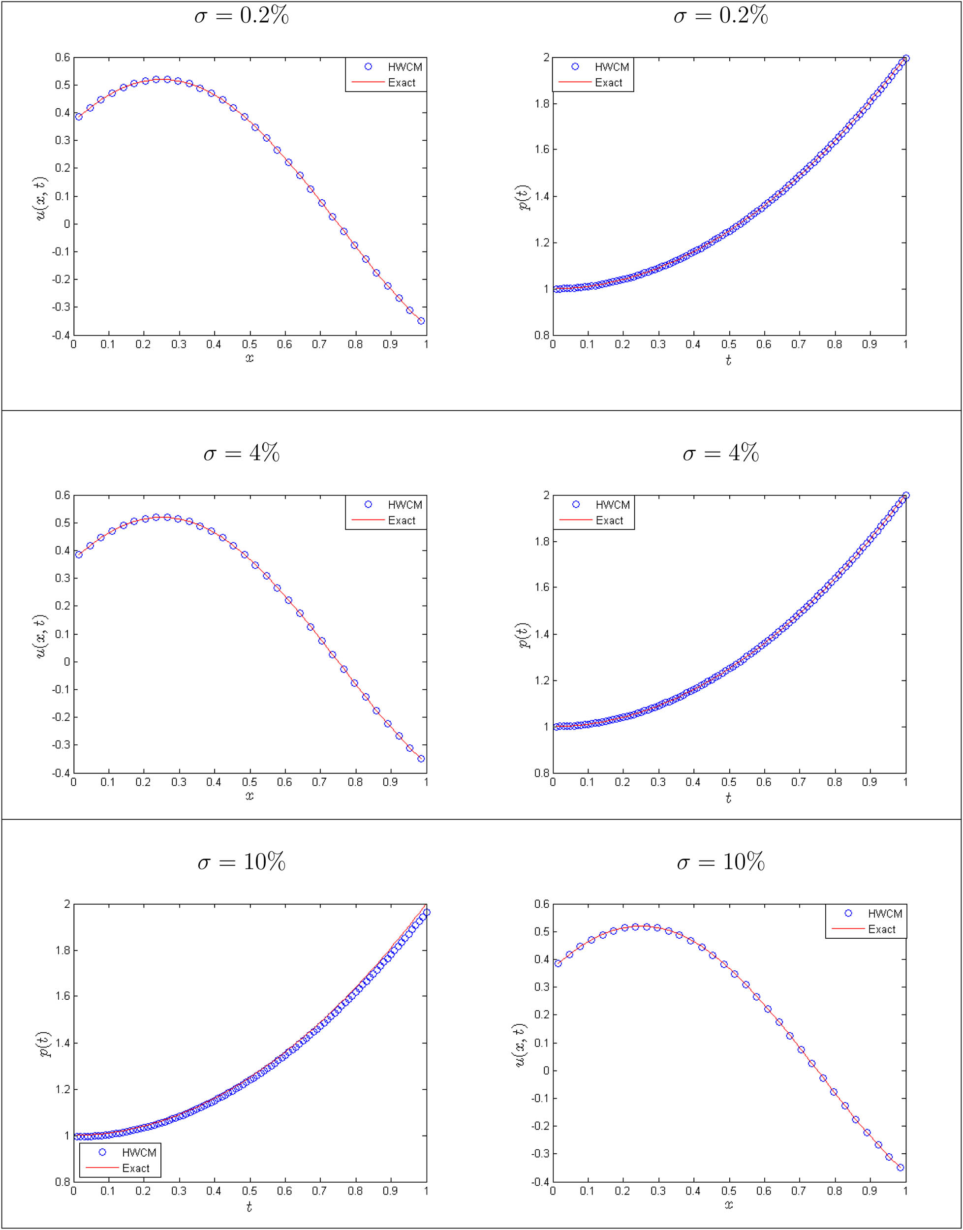
Comparison of numerical results with different

The absolute values of the errors with different
Example 2
Consider the IHCP along with the following input data
The exact solution
Figure 4 depicts comparison of results of the established method with the analytical solution at

Comparison of numerical results for Example 2 at

Comparison of numerical results for Example 2 at
The flexibility of the proposed HWCM for the oscillatory type numerical solution of

Comparison of exact and numerical results for Example 2 at

The absolute values of the errors with different

The 3D overview of the numerical solutions at
6 Conclusion
In this article, a multi-resolution HWCM is adopted for a time-dependent inverse problem focused on diffusion equation with source control parameter. The propped method is stable and convergent. It is the advantage of the HWCM that convert the ill-posed PDE into a well-condition system of equation and hence no need to introduced any regularization procedure. The numerical results of the examples are in line with the theoretical discussion. The accuracy, stability, and efficiency are due to the well-condition system matrix. The HWCM can also produce stable results for the inverse problem under a large intensity of noise level (
-
Funding information: This research was supported by the Project of Guangdong Provincial Department of Education Under No. 2020WQNCX049.
-
Author contributions: All authors have accepted responsibility for the entire content of this manuscript and approved its submission.
-
Conflict of interest: The authors state no conflict of interest.
References
[1] Dehghan M. Finding a control parameter in one-dimensional parabolic equations. Appl Math Comput. 2003;135(2–3):491–503. 10.1016/S0096-3003(02)00063-2Search in Google Scholar
[2] Ye C, Sun Z. On the stability and convergence of a difference scheme for an one-dimensional parabolic inverse problem. Appl Math Comp. 2007;188(1):214–25. 10.1016/j.amc.2006.09.109Search in Google Scholar
[3] Liu C-S. A double optimal descent algorithm for iteratively solving ill-posed linear inverse problems. Inverse Probl Sci Eng. 2015;23(1):38–66. 10.1080/17415977.2014.880905Search in Google Scholar
[4] Liu C-S. A highly accurate LGSM for severely ill-posed BHCP under a large noise on the final time data. Int J Heat Mass Transfer. 2010;53(19–20):4132–40. 10.1016/j.ijheatmasstransfer.2010.05.036Search in Google Scholar
[5] Tariq M, Ahmad H, Sahoo SK. The Hermite-Hadamard type inequality and its estimations via generalized convex functions of Raina type. Math Model Numer Simulat Appl (MMNSA). 2021;1(1):32–43. 10.53391/mmnsa.2021.01.004Search in Google Scholar
[6] Akbar MA, Akinyemi L, Yao S-W, Jhangeer A, Rezazadeh H, Khater MM, et al. Soliton solutions to the boussinesq equation through sine-gordon method and kudryashov method. Results Phys. 2021;25:104228. 10.1016/j.rinp.2021.104228Search in Google Scholar
[7] Ahmad I, Ahsan M, Hussain I, Kumam P, Kumam W. Numerical simulation of PDEs by local meshless differential quadrature collocation method. Symmetry. 2019;11(3):394. 10.3390/sym11030394Search in Google Scholar
[8] Ahmad I, Ahmad H, Inc M, Rezazadeh H, Akbar MA, Khater MM, et al. Solution of fractional-order Korteweg-de Vries and burgers equations utilizing local meshless method. J Ocean Eng Sci. 10.1016/j.joes.2021.08.014. Search in Google Scholar
[9] Ahmad I, Ahsan M, Din Z-u, Masood A, Kumam P. An efficient local formulation for time-dependent PDEs. Mathematics. 2019;7(3):216. 10.3390/math7030216Search in Google Scholar
[10] Wang F, Zhang J, Ahmad I, Farooq A, Ahmad H. A novel meshfree strategy for a viscous wave equation with variable coefficients. Front Phys. 2021;9:359. 10.3389/fphy.2021.701512Search in Google Scholar
[11] Akinyemi L, Rezazadeh H, Yao S-W, Akbar MA, Khater MM, Jhangeer A, et al. Nonlinear dispersion in parabolic law medium and its optical solitons. Results Phys. 2021:104411. 10.1016/j.rinp.2021.104411Search in Google Scholar
[12] Avci D, Yavuz M, Ozdemir N. Fundamental solutions to the Cauchy and Dirichlet problems for a heat conduction equation equipped with the Caputo-Fabrizio differentiation. in: Heat Conduction: Methods, Applications and Research. Hauppauge, New York, USA: NOVA Science Publishers; 2019. p. 95–107. Search in Google Scholar
[13] Yavuz M, Özdemir N. Numerical inverse Laplace homotopy technique for fractional heat equations. Thermal Sci 2018;22(1):85–194. 10.2298/TSCI170804285YSearch in Google Scholar
[14] Akgül EK, Akgül A, Yuvuz M. New illustrative applications of integral transforms to financial models with different fractional derivatives. Chaos Soliton Fractal. 2021;146:110877. 10.1016/j.chaos.2021.110877Search in Google Scholar
[15] Akinyemi L, Rezazadeh H, Shi Q-H, Inc M, Khater MM, Ahmad H, et al. New optical solitons of perturbed nonlinear schrödinger-hirota equation with spatio-temporal dispersion. Results Phys. 2021;29:104656. 10.1016/j.rinp.2021.104656Search in Google Scholar
[16] Yokus A, Yavuz M. Novel comparison of numerical and analytical methods for fractional Burger-Fisher equation. Discrete Contin Dyn Syst-S 2021;14(7):2591. 10.3934/dcdss.2020258Search in Google Scholar
[17] Ahmad H, Khan TA, Ahmad I, Stanimirović PS, Chu Y-M. A new analyzing technique for nonlinear time fractional Cauchy reaction-diffusion model equations. Results Phys. 2020;19:103462. 10.1016/j.rinp.2020.103462Search in Google Scholar
[18] Ahmad I, Ahmad H, Thounthong P, Chu Y-M, Cesarano C. Solution of multi-term time-fractional PDE models arising in mathematical biology and physics by local meshless method. Symmetry. 2020;12(7):1195. 10.3390/sym12071195Search in Google Scholar
[19] Cannon J, Lin Y, Xu S. Numerical procedures for the determination of an unknown coefficient in semi-linear parabolic differential equations. Inverse Problems. 1994;10(2):227. 10.1088/0266-5611/10/2/004Search in Google Scholar
[20] Yan L, Fu C-L, Yang F-L. The method of fundamental solutions for the inverse heat problem. Eng Anal Bound Elem. 2008;32:216–22. 10.1016/j.enganabound.2007.08.002Search in Google Scholar
[21] Farcas A, Lesnic D. The boundary-element method for the determination of a heat source dependent on one variable. J Eng Math. 2006;54(4):375–88. 10.1007/s10665-005-9023-0Search in Google Scholar
[22] Liu C-S. An iterative algorithm for identifying heat source by using a DQ and a Lie-group method. Inverse Probl Sci Eng. 2015;23(1):67–92. 10.1080/17415977.2014.880907Search in Google Scholar
[23] Liu C-S. Lie-group differential algebraic equations method to recover heat source in a Cauchy problem with analytic continuation data. Int J Heat Mass Transfer. 2014;78:538–47. 10.1016/j.ijheatmasstransfer.2014.07.010Search in Google Scholar
[24] Kuo C-L, Liu C-S, Chang J-R. The modified polynomial expansion method for identifying the time dependent heat source in two-dimensional heat conduction problems. Int J Heat Mass Transfer. 2016;92:658–64. 10.1016/j.ijheatmasstransfer.2015.09.025Search in Google Scholar
[25] NawazKhan M, Ahmad I, Ahmad H. A radial basis function collocation method for space-dependent inverse heat problems. J Appl Comput Mech. 2020;6(Special Issue):1187–99. Search in Google Scholar
[26] Khan MN, Hussain I, Ahmad I, Ahmad H. A local meshless method for the numerical solution of space-dependent inverse heat problems. Math Meth Appl Sci. 2021;44(4):3066–79. 10.1002/mma.6439Search in Google Scholar
[27] Aziz I, Siraj-ul-Islam, Nisar M. An efficient numerical algorithm based on Haar wavelet for solving a class of linear and nonlinear nonlocal boundary-value problems. Calcolo. 2016;53(4):621–33. 10.1007/s10092-015-0165-9Search in Google Scholar
[28] Siraj-ul-Islam, Ahsan M, Hussian I. A multi-resolution collocation procedure for time-dependent inverse heat problems. Int J Therm Sci. 2018;128:160–74. 10.1016/j.ijthermalsci.2018.01.001Search in Google Scholar
[29] Ahsan M, Siraj-ul-Islam, Hussain I. Haar wavelets multi-resolution collocation analysis of unsteady inverse heat problems. Inverse Probl Sci Eng. 2019;27:1498–520. 10.1080/17415977.2018.1481405Search in Google Scholar
[30] Ahsan M, Ahmad I, Ahmad M, Hussian I. A numerical Haar wavelet-finite difference hybrid method for linear and non-linear schrödinger equation. Math Comp Simulat. 2019;165:13–25. 10.1016/j.matcom.2019.02.011Search in Google Scholar
[31] Mallat S. A wavelet tour of signal processing: the sparse way. Burlington, MA: Academic Press; 2008. Search in Google Scholar
[32] Liu Y, Liu Y, Cen Z. Daubechies wavelet meshless method for 2-D elastic problems. Tsinghua Sci Technol. 2008;13(5):605–8. 10.1016/S1007-0214(08)70099-3Search in Google Scholar
[33] Siraj-ul-Islam, Aziz I, Ahmad M. Numerical solution of two-dimensional elliptic PDEs with nonlocal boundary conditions. Comp Math Appl. 2015;69(3):180–205. 10.1016/j.camwa.2014.12.003Search in Google Scholar
[34] Jang G-W, Kim YY, Choi KK. Remesh-free shape optimization using the wavelet-Galerkin method. Int J Solids Struct. 2004;41(22):6465–83. 10.1016/j.ijsolstr.2004.05.010Search in Google Scholar
[35] Díaz LA, Martín MT, Vampa V. Daubechies wavelet beam and plate finite elements. Finite Elem Anal Des. 2009;45(3):200–9. 10.1016/j.finel.2008.09.006Search in Google Scholar
[36] Abdeljawad T, Amin R, Shah K, Al-Mdallal Q, Jarad F. Efficient sustainable algorithm for numerical solutions of systems of fractional order differential equations by Haar wavelet collocation method. Alexandria Eng J. 2020;59(4):2391–400. 10.1016/j.aej.2020.02.035Search in Google Scholar
[37] Rawat S. Quality assessment in image compression by using fast wavelet transformation with 2D Haar wavelets. Int Res J Eng Technol. 2017;4(5):508–18. Search in Google Scholar
[38] Belkadhi K, Elhamdi K, Bhar M, Manai K. Dose calculation using Haar wavelets with buildup correction. Appl Radiat Isotopes. 2017;127:186–94. 10.1016/j.apradiso.2017.06.011Search in Google Scholar PubMed
[39] Fryzlewicz P, Timmermans C. Shah: Shape-Adaptive Haar wavelets for image processing. J Comput Graph Statist. 2016;25(3):879–98. 10.1080/10618600.2015.1048345Search in Google Scholar
[40] Feklistova L, Hein H. Delamination identification using machine learning methods and Haar wavelets. Comp Assist Methods Eng Sci. 2017;19(4):351–60. Search in Google Scholar
[41] Vaidelienė G, Valantinas J. The use of Haar wavelets in detecting and localizing texture defects. Image Anal Stereol. 2016;35(3):195–201. 10.5566/ias.1561Search in Google Scholar
[42] Lefebvre A, Liu J, Mueller E, Nadar MS, Schmidt M, Zenge M, et al. MRI reconstruction with incoherent sampling and redundant Haar wavelets. US Patent No 9,396,562. Jul. 19 2016. Search in Google Scholar
[43] Nazir S, Shahzad S, Wirza R, Amin R, Ahsan M, Mukhtar N, et al. Birthmark based identification of software piracy using haar wavelet. Math Comp Simulat. 2019;166:144–54. 10.1016/j.matcom.2019.04.010Search in Google Scholar
[44] McMorris D, Pearson P, Yurk B. A modified wavelet method for identifying transient features in time signals with applications to bean beetle maturation. Involve J Math. 2016;10(1):21–42. 10.2140/involve.2017.10.21Search in Google Scholar
[45] Majak J, Shvartsman B, Kirs M, Pohlak M, Herranen H. Convergence theorem for the Haar wavelet-based discretization method. Composite Struct. 2015;126:227–32. 10.1016/j.compstruct.2015.02.050Search in Google Scholar
[46] Kumar M, Pandit S. A composite numerical scheme for the numerical simulation of coupled burgers equation. Comp Phys Commun. 2014;185(3):809–17. 10.1016/j.cpc.2013.11.012Search in Google Scholar
© 2021 Muhammad Ahsan et al., published by De Gruyter
This work is licensed under the Creative Commons Attribution 4.0 International License.
Articles in the same Issue
- Regular Articles
- Circular Rydberg states of helium atoms or helium-like ions in a high-frequency laser field
- Closed-form solutions and conservation laws of a generalized Hirota–Satsuma coupled KdV system of fluid mechanics
- W-Chirped optical solitons and modulation instability analysis of Chen–Lee–Liu equation in optical monomode fibres
- The problem of a hydrogen atom in a cavity: Oscillator representation solution versus analytic solution
- An analytical model for the Maxwell radiation field in an axially symmetric galaxy
- Utilization of updated version of heat flux model for the radiative flow of a non-Newtonian material under Joule heating: OHAM application
- Verification of the accommodative responses in viewing an on-axis analog reflection hologram
- Irreversibility as thermodynamic time
- A self-adaptive prescription dose optimization algorithm for radiotherapy
- Algebraic computational methods for solving three nonlinear vital models fractional in mathematical physics
- The diffusion mechanism of the application of intelligent manufacturing in SMEs model based on cellular automata
- Numerical analysis of free convection from a spinning cone with variable wall temperature and pressure work effect using MD-BSQLM
- Numerical simulation of hydrodynamic oscillation of side-by-side double-floating-system with a narrow gap in waves
- Closed-form solutions for the Schrödinger wave equation with non-solvable potentials: A perturbation approach
- Study of dynamic pressure on the packer for deep-water perforation
- Ultrafast dephasing in hydrogen-bonded pyridine–water mixtures
- Crystallization law of karst water in tunnel drainage system based on DBL theory
- Position-dependent finite symmetric mass harmonic like oscillator: Classical and quantum mechanical study
- Application of Fibonacci heap to fast marching method
- An analytical investigation of the mixed convective Casson fluid flow past a yawed cylinder with heat transfer analysis
- Considering the effect of optical attenuation on photon-enhanced thermionic emission converter of the practical structure
- Fractal calculation method of friction parameters: Surface morphology and load of galvanized sheet
- Charge identification of fragments with the emulsion spectrometer of the FOOT experiment
- Quantization of fractional harmonic oscillator using creation and annihilation operators
- Scaling law for velocity of domino toppling motion in curved paths
- Frequency synchronization detection method based on adaptive frequency standard tracking
- Application of common reflection surface (CRS) to velocity variation with azimuth (VVAz) inversion of the relatively narrow azimuth 3D seismic land data
- Study on the adaptability of binary flooding in a certain oil field
- CompVision: An open-source five-compartmental software for biokinetic simulations
- An electrically switchable wideband metamaterial absorber based on graphene at P band
- Effect of annealing temperature on the interface state density of n-ZnO nanorod/p-Si heterojunction diodes
- A facile fabrication of superhydrophobic and superoleophilic adsorption material 5A zeolite for oil–water separation with potential use in floating oil
- Shannon entropy for Feinberg–Horodecki equation and thermal properties of improved Wei potential model
- Hopf bifurcation analysis for liquid-filled Gyrostat chaotic system and design of a novel technique to control slosh in spacecrafts
- Optical properties of two-dimensional two-electron quantum dot in parabolic confinement
- Optical solitons via the collective variable method for the classical and perturbed Chen–Lee–Liu equations
- Stratified heat transfer of magneto-tangent hyperbolic bio-nanofluid flow with gyrotactic microorganisms: Keller-Box solution technique
- Analysis of the structure and properties of triangular composite light-screen targets
- Magnetic charged particles of optical spherical antiferromagnetic model with fractional system
- Study on acoustic radiation response characteristics of sound barriers
- The tribological properties of single-layer hybrid PTFE/Nomex fabric/phenolic resin composites underwater
- Research on maintenance spare parts requirement prediction based on LSTM recurrent neural network
- Quantum computing simulation of the hydrogen molecular ground-state energies with limited resources
- A DFT study on the molecular properties of synthetic ester under the electric field
- Construction of abundant novel analytical solutions of the space–time fractional nonlinear generalized equal width model via Riemann–Liouville derivative with application of mathematical methods
- Some common and dynamic properties of logarithmic Pareto distribution with applications
- Soliton structures in optical fiber communications with Kundu–Mukherjee–Naskar model
- Fractional modeling of COVID-19 epidemic model with harmonic mean type incidence rate
- Liquid metal-based metamaterial with high-temperature sensitivity: Design and computational study
- Biosynthesis and characterization of Saudi propolis-mediated silver nanoparticles and their biological properties
- New trigonometric B-spline approximation for numerical investigation of the regularized long-wave equation
- Modal characteristics of harmonic gear transmission flexspline based on orthogonal design method
- Revisiting the Reynolds-averaged Navier–Stokes equations
- Time-periodic pulse electroosmotic flow of Jeffreys fluids through a microannulus
- Exact wave solutions of the nonlinear Rosenau equation using an analytical method
- Computational examination of Jeffrey nanofluid through a stretchable surface employing Tiwari and Das model
- Numerical analysis of a single-mode microring resonator on a YAG-on-insulator
- Review Articles
- Double-layer coating using MHD flow of third-grade fluid with Hall current and heat source/sink
- Analysis of aeromagnetic filtering techniques in locating the primary target in sedimentary terrain: A review
- Rapid Communications
- Nonlinear fitting of multi-compartmental data using Hooke and Jeeves direct search method
- Effect of buried depth on thermal performance of a vertical U-tube underground heat exchanger
- Knocking characteristics of a high pressure direct injection natural gas engine operating in stratified combustion mode
- What dominates heat transfer performance of a double-pipe heat exchanger
- Special Issue on Future challenges of advanced computational modeling on nonlinear physical phenomena - Part II
- Lump, lump-one stripe, multiwave and breather solutions for the Hunter–Saxton equation
- New quantum integral inequalities for some new classes of generalized ψ-convex functions and their scope in physical systems
- Computational fluid dynamic simulations and heat transfer characteristic comparisons of various arc-baffled channels
- Gaussian radial basis functions method for linear and nonlinear convection–diffusion models in physical phenomena
- Investigation of interactional phenomena and multi wave solutions of the quantum hydrodynamic Zakharov–Kuznetsov model
- On the optical solutions to nonlinear Schrödinger equation with second-order spatiotemporal dispersion
- Analysis of couple stress fluid flow with variable viscosity using two homotopy-based methods
- Quantum estimates in two variable forms for Simpson-type inequalities considering generalized Ψ-convex functions with applications
- Series solution to fractional contact problem using Caputo’s derivative
- Solitary wave solutions of the ionic currents along microtubule dynamical equations via analytical mathematical method
- Thermo-viscoelastic orthotropic constraint cylindrical cavity with variable thermal properties heated by laser pulse via the MGT thermoelasticity model
- Theoretical and experimental clues to a flux of Doppler transformation energies during processes with energy conservation
- On solitons: Propagation of shallow water waves for the fifth-order KdV hierarchy integrable equation
- Special Issue on Transport phenomena and thermal analysis in micro/nano-scale structure surfaces - Part II
- Numerical study on heat transfer and flow characteristics of nanofluids in a circular tube with trapezoid ribs
- Experimental and numerical study of heat transfer and flow characteristics with different placement of the multi-deck display cabinet in supermarket
- Thermal-hydraulic performance prediction of two new heat exchangers using RBF based on different DOE
- Diesel engine waste heat recovery system comprehensive optimization based on system and heat exchanger simulation
- Load forecasting of refrigerated display cabinet based on CEEMD–IPSO–LSTM combined model
- Investigation on subcooled flow boiling heat transfer characteristics in ICE-like conditions
- Research on materials of solar selective absorption coating based on the first principle
- Experimental study on enhancement characteristics of steam/nitrogen condensation inside horizontal multi-start helical channels
- Special Issue on Novel Numerical and Analytical Techniques for Fractional Nonlinear Schrodinger Type - Part I
- Numerical exploration of thin film flow of MHD pseudo-plastic fluid in fractional space: Utilization of fractional calculus approach
- A Haar wavelet-based scheme for finding the control parameter in nonlinear inverse heat conduction equation
- Stable novel and accurate solitary wave solutions of an integrable equation: Qiao model
- Novel soliton solutions to the Atangana–Baleanu fractional system of equations for the ISALWs
- On the oscillation of nonlinear delay differential equations and their applications
- Abundant stable novel solutions of fractional-order epidemic model along with saturated treatment and disease transmission
- Fully Legendre spectral collocation technique for stochastic heat equations
- Special Issue on 5th International Conference on Mechanics, Mathematics and Applied Physics (2021)
- Residual service life of erbium-modified AM50 magnesium alloy under corrosion and stress environment
- Special Issue on Advanced Topics on the Modelling and Assessment of Complicated Physical Phenomena - Part I
- Diverse wave propagation in shallow water waves with the Kadomtsev–Petviashvili–Benjamin–Bona–Mahony and Benney–Luke integrable models
- Intensification of thermal stratification on dissipative chemically heating fluid with cross-diffusion and magnetic field over a wedge