A real negative selection algorithm with evolutionary preference for anomaly detection
-
Tao Yang
 and
Tao Li
and
Tao Li

Abstract
Traditional real negative selection algorithms (RNSAs) adopt the estimated coverage (c0) as the algorithm termination threshold, and generate detectors randomly. With increasing dimensions, the data samples could reside in the low-dimensional subspace, so that the traditional detectors cannot effectively distinguish these samples. Furthermore, in high-dimensional feature space, c0 cannot exactly reflect the detectors set coverage rate for the nonself space, and it could lead the algorithm to be terminated unexpectedly when the number of detectors is insufficient. These shortcomings make the traditional RNSAs to perform poorly in high-dimensional feature space. Based upon “evolutionary preference” theory in immunology, this paper presents a real negative selection algorithm with evolutionary preference (RNSAP). RNSAP utilizes the “unknown nonself space”, “low-dimensional target subspace” and “known nonself feature” as the evolutionary preference to guide the generation of detectors, thus ensuring the detectors can cover the nonself space more effectively. Besides, RNSAP uses redundancy to replace c0 as the termination threshold, in this way RNSAP can generate adequate detectors under a proper convergence rate. The theoretical analysis and experimental result demonstrate that, compared to the classical RNSA (V-detector), RNSAP can achieve a higher detection rate, but with less detectors and computing cost.
1 Introduction
Biological Immune System (BIS) can distinguish between self-organization and harmful antigens, and eliminate harmful antigens to ensure biology in health. Inspiration by BIS, formed the research field of Artificial Immune System (AIS) which has attracted more and more researchers to develop many algorithms. In AIS, the Negative Selection Algorithm (NSA) is an important detector generating algorithm which was first proposed by Forrest et al. [1]. The NSA simulates the T cells censoring process in the thymus to generate mature detectors without immune Self-Reaction. It has shown to be efficient for anomaly detection [2, 3], data classification and fault diagnosis [4, 5].
Early negative selection algorithms defined the antibody (detector) and antigen (abnormal data) in binary representation, and used R-Continue-Bits Match Rule to calculate affinity of antibody and antigen [1]. On account of the fact that many applications are natural to be described in real-valued feature space, Gonzalez and Dasgupta proposed a Real Negative Selection Algorithm (RNSA) [6], in which the data samples (detectors and antigens) are normalized into the real-valued feature space [0, 1]n (n denotes the number of samples dimension), and the affinity is calculated by the Minkowski distance. Some modified versions of RNSA have been proposed, Ji and Dasgupta proposed Real Negative Selection Algorithm with variable detector radius (V-detector) [7], in which the detector radius was dynamically resized to the nearest selfmargin; Gong presented a further training method to reduce the computational expense by reducing the self samples [8]; Chen improved the detectors generation efficiency by adopting the hierarchical clustering preprocess of self set [1]; Poggiolini implicated the feature detection rule to RNSA and improved the algorithm performance [10].
The major challenge of NSA is to efficiently generate effective detectors. Traditional RNSA generates detectors randomly, until the Estimated Coverage (c0) reaches the threshold. In high-dimensional feature space, the distribution of samples is extremely sparse and non-uniform, in that case c0 could not exactly reflect the coverage for nonself samples, leading the algorithms converge so fast that it is terminated unexpectedly while there only a few detectors generated. Besides, in high-dimension, a large number of data samples could “fall” into the subspace, the conventional detectors cannot discriminate these samples without appropriate guidance. These shortcomings cause the traditional negative selection algorithm to perform poorly in high-dimensions feature space, and restrict the application of artificial immune theory in anomaly detection.
The evolution of the immune cell has the evolutionary preference to capture the pathogen antigen. Following from this, this paper proposes a real negative selection algorithm with evolutionary preference (RNSAP) which uses a novel termination condition and a new detector training strategy. First, for guaranteeing the detectors can cover more nonself space and reduce the redundant detectors, RNSAP adds the preference of “cover unknown nonself space” to the conventional detectors by applying redundancy testing, and then uses the redundancy (R) as an algorithm termination threshold to ensure the algorithm is convergent under a prober rate. Second, to effectively cover the low-dimensional subspace where samples might gather in, RNSAP will calculate out the “low-dimensional target subspace” and utilize it as the “spatial preference” to generate the detectors with spatial preference. Lastly, for excluding the “hole” as much as possible, RNSAP will use the “known nonself sample” as “feature preference” to train detectors with feature preference. The theoretical analysis and experimental results suggest: compared to a classical real negative selection algorithm (V-detector) on low-dimension dataset (Haberman's Survival Data Set), RNSAP has a higher detection rate, with fewer detectors and shorter training time; on high-dimension dataset (KDD CUP99), the performance of traditional NSA is very poor while RNSAP performs well.
The rest of this paper is organized as follows: In Section 2, some basic definition are covered; In Section 3 RNSAP is introduced in detail; Experiment results are shown and discussed in Section 4 while Concluding remarks are given in Section 5.
2 Basic definition
The immune system relies on antibody cell discrimination “self” and “nonself” exclude antigenicity, is human's primacy defense against pathogenic organisms and cells. In an Artificial Immune System, data samples are defined as “antigen”, normal samples are defined as “self”, abnormal samples are defined as “nonself”, and antibody is defined as “detector”. For faciliting the description, define the basic conceptions of RNSAP as follows:
Definition 1 (antigen)
All the character strings abstracted from the feature space constitute the antigen set U = {g|(f1, f2, …, fn), fi ∈ [0,1]}, where n is the data dimension and fi represents the i-th normalized attribute value.
Definition 2 (self/nonself set)
The self set S ⊂ U is the character strings abstracted from normal samples, rs ∈ R+ is the variability threshold of the self sample; Nonself set N = U – S, which represents character strings abstracted from abnormal samples, and S ⋃ N = U, S ⋂ N = Φ.
Definition 3 (detector)
Detector d = (c, r), where c ∈ N, c is the central vector of d in the feature space; r ∈ R+ is the detector radius. Antigens which are close to any detector less than r will be identified as nonself elements.
Definition 4 (self-reactive)
If any self element located in the detection region of detector d, and then d is a self-reactive detector.
Definition 5 (self/nonself space)
In feature space, the part of being covered by self samples is called self space, the rest of space is nonself space; in the nonself space, the part of being covered by detectors is called known nonself space while the remaining part is unknown nonself space.
3 The strategies of RNSAP
The main idea of RNSAP is using the redundancy (R) to replace the estimated coverage (c0) as the termination threshold, and utilizes the “unknown nonself space”, “low-dimensional target subspace” and “known nonself feature” as the evolutionary preference to guide the generation of detectors. In that way, RNSAP can generate more effective detectors with the proper rate of convergence.
3.1 The termination condition of detector generation in RNSAP
3.1.1 The influence of dimension on estimated coverage
In a traditional real negative selection algorithm, the coverage rate of detector set for nonself space (p) determines the performance of immune algorithm, and p can be expressed as:
Because Eq. 1 is difficult to calculate directly, paper [7] proposed a method to evaluate P by using “point estimate”:
In Eq. 2, t is the times of without finding an uncovered random point, and c0 is the Estimated Coverage. If c0 = 80%, the algorithm will be terminated when continuous find 5 random sampling covered by the detectors set.
After normalisation, the n-dimensional feature space is represented as n-dimensional hypercube u = [0,1]n, the data samples are represented as the “points” and the detectors are represented the “hyper-sphere”. The c0 represents the coverage situation between “data sample” (point) and “detector” (hyper-sphere). In low-dimension space, if the training samples are distributed uniformly, c0 can reflect the real coverage rate of detector set for non-self space. However, if training samples are non-uniformly distributed, the c0 will no longer apply.
Comparison of Fig. 1(a) and Fig. 1(b) reveals that, Fig. 1(a) has 7 self samples (green “.”) and 10 nonself samples (red “+”) uniform distributed in 2-dimensional feature space, the 12 mature detectors cover almost whole 2-d space; While Fig. 1(b) only has 1 self sample and 1 nonself sample distributed in edge of space (sparse and non-uniform), the 1 big mature detector covers almost the whole 2-d space. Fig. 1 shows that the mature detectors have covered almost all feature space, so the Eq. 2 would be easy to meet (assume c0 = 80%). However in Fig. 1(a) the real coverage rate on this training set is 90% and in Fig. 1(b) is 0.

The influence of sample distribution on detectors generation
In high-dimensional space the samples distribution is always sparsely and non-uniform [11]. Firstly, assuming in n-dimensional feature, the value range of data samples on i-th dimension is [0, ni], and then the total amount of data (Na) that n-dimensional feature space could accommodate is:
From Eq. 3, Na grows exponentially with the n, and the number of training data (Nt) is limited by the data set and is customarily much smaller than Na, so the training data distribution may extremely sparsely in high-dimensional feature space.
Secondly the unitary hypercube u = [0, 1]n has a total volume of 1, assume u0 is one other n-dimensional hypercube inside u, then the volume of u0 is:
where a is the side length of the cube u0, a ∈ [0,1). From Eq. 4, if a = 0.9 and n = 40, Vu0 is approximately 0.015, that means the u0 (the central part of u) only contains 1.5% samples (assuming a plenty of samples uniform distribute in the u and fill the whole space), and about 98.5% samples locate in the edge marginal area of u. In contrast, the n-dimensional detectors (hyper-sphere) with a variable radius
3.1.2 The redundancy and redundant testing
In fact, the coverage situation between “mature detector” (hyper-sphere) and “candidate detector” (hyper-sphere) is calculated more easily and it is not influenced by the dimension growth. If the most volume of a candidate detector (di) overlaps with a mature detector (dm), the (di) could be considered as a “redundant detector”. When there are too many redundant detectors in feature space, randomly generated detectors cannot guarantee that the new mature detectors cover the unknown nonself space. In that case, considering the efficiency and performance, the generation of detectors should been terminated. Thus RNSAP adopts the redundancy (R) as the algorithm termination threshold.
For calculating redundancy R, RNSAP divide the “Redundant-Judgment Zone” by using detector radius (r), detector central vector (c) and distant parameters. As shown in Fig. 2(a), the gray zone is the “redundant-judgment zone” which depends on dm = <cm, rm> (the mature detectors), sm (the most vicinity self-sample of dm) and a variable parameter Rc ∈ [0.1]. If a new candidate detector dn = <cn, rn> locates in the redundant-judgment zone (dn satisfy with expression 5), dn should be judged as a redundant detector and be removed, and the redundant count will be accumulated:
In expression 5, lns is the Euclid distant between cn and sm, lmn is the Euclid distant between cn and cm. Rc ∈ [0,1] is variable parameter, the size of redundant-judgment zone is proportional to Rc. If Rc is close to 0, the size of redundant-judgment zone is smaller, the probability of dn being judged as a redundant detector is lower, the feature space could accommodate more detectors. If Rc is close to 1 the size of redundant-judgment zone is larger, and the probability of dn being judged as a redundant detector is higher, the feature space could accommodate less detectors.
Fig. 2(b), Fig. 2(c) and Fig. 2(d) show the process of redundancy testing. The testing uses the same dm and the redundant-judgment zone (gray zone). In Fig. 2(b) candidate detector dn1 locates in the redundant-judgment zone, its volume almost overlapping of mature detector dm, so dn1 should be judged as a redundant detector; In Fig. 2(c) and Fig. 2(d), dn2 and dn3 do not locate in redundant-judgment zone, their volume is just partially covered by dm, compare to dn1 they can cover more known nonself space, thus dn2 and dn3 will become the new mature detector.

Redundant-judgment zone and redundant testing
In each round of redundancy testing, if a candidate detector is judged as a redundant detector, the RNSAP will accumulate the “redundant count” (cnt), then calculate the ratio (redundancy R) of cnt and amount of mature detectors (Nm):
If R reaches the threshold, it means in the last round there were too many redundant detectors. In this situation, obtaining new high quantity (ir-redundant) detectors becomes more difficult, considering the efficiency and performance, RNSAP will terminate the random generation of detectors.
Different from estimate coverage (c0), redundant testing calculates the cover situation between “mature detector” (hyper-sphere) and “candidate detector” (hyper-sphere). It has nothing to do with data distribution, so it is available in high-dimensional space. There are two obvious advantages in using the redundancy (R) as the termination threshold: 1. it can ensure the algorithm is convergent under a proper rate; 2. by using condition (5) RNSAP adds a preference of “cover unknown nonself space” to the randomly generation process of detectors, therefore the redundant testing not only removes the redundant detectors but also improves the quality of detectors.
RNSAP calls the detectors which are randomly generated as a conventional detector, the conventional detectors generation algorithm by using redundant testing as shown in Table 1.
The generation of conventional detectors
|
3.2 The detectors with evolutionary preference
Despite that conventional detectors have been highly redundant in feature space, there might be still some “uncovered nonself space” left. Completely random generation of detectors to cover the uncovered nonself space will cost too many of computing resources. Perelson proposed the Immune Repertoire Model and pointed out that “not all receptor shapes (detectors) need to be made at random” [12]. The latest immunology research results show that: The evolution of Immune cell is not entirely a random process, but rather has an evolutionary preference to capture the pathogen antigen [13]. Based on these theories, RNSAP utilizes the “low-dimensional target subspace” and “known nonself feature” as the evolutionary preference to guide the generation of detectors. The detectors with preference can effectively cover reducing the uncovered nonself space and improve the performance of algorithm significantly.
3.2.1 The detectors with spatial preference
In high-dimension feature space, the training samples would fall into the low-dimension subspace. As shown in Fig. 3(a)(Haberman's Survival dataset), in the 3-dimension (XYZ) feature space, the green ’.’ represents self sample, the red ’+’ represents nonself sample, the 3D-sphere represents mature conventional detector generated by V-detector algorithm, (rs = 0.01, c0 = 90%). There are many samples falling into the “XY plane”, however only a few mature detectors (such as di and dj ) intersect with the XY plane. The Fig. 3(b) shows the coverage of mature detectors for the XY subspace from XY-perspective, the conventional detectors are almost not cover the nonself samples in XY subspace. The most effective way to distinguish these samples which fall into the subspace is to generate detectors in the aimed subspace, in other words the central vector (c) of candidate detector should locate in the aimed subspace directly. When the one dimension of data get 0 value, the data would fall into the corresponding subspace, assuming Pi_0 represents the probability of the ith dimension of c gets 0 value, then the probability (Pj…k) of the any candidate detectors’ central vector fall into the subspace Sj…k is:

The convention detectors (V-detector)
From the Eq. 7, Pj…k becomes lower when n growth, so in the high-dimension space it is almost impossible for candidate detectors to cover the subspace by random generation. To deal with this situation, RNSAP analyzes the distribution of the training sample first; and then find out all the “target subspaces” which have high density of samples; at last use “target subspaces” as spatial preference to guide the generation of the detector.
For a single dimension, the density of data distribution can be described by a Jini value [12]. The Jini value of dimension A can be calculated by Eq. 8:
Where ω is the number of equal interval (the “0” is treated a single interval) which is divided in the dimension A, pi is the proportion of the number of samples which located in the ith interval to the total number. From Eq. 8, the smaller Jini value indicates that the distribution of samples is more densely in the dimension A while the larger Jini value indicates the distribution is more dispersed. By calculating the Jini value and presetting the Jini threshold ξ, RNSAP can select out all the dimension in which the distribution of samples is dense. And then, RNSAP will calculate out the cluster center χ in each dense dimension. At last, the χ will be used to edit the central vector c.
In expression 9, ci denotes the ith dimension value of central vector c. RNSAP according three cases to set the value of ci: (1) If dimension A is a dense dimension and samples in A gather in “0”, RNSAP sets the ci = 0 for that the candidate detectors will be generated in the low-dimension subspace. (2) If dimension A is a dense dimension and samples gather in χ (χ ≠ 0), ci will take a random value between χ-θ and χ+θ, for that the candidate detectors will be generated in the region where samples distribute dense. (3) If dimension A is not a densely dimension, A cannot provide any spatial information to guide the generation of detector, ci will take a random value between [0, 1] as conventional algorithm.
By using expression 9, RNSAP can generate the detector with spatial preference in the target subspace accurately. The detectors with spatial preference are shown in Fig. 4(a) and Fig. 4(b) (for the convenience of observation, all the conventional detectors are not shown). Compare Fig. 3(b) with Fig. 4(b), in XY subspace conventional detectors could barely recognize nonself samples while by training the detectors with spatial preference RNSAP almost covered all nonself samples. It is worthy to notice that: different from the dimension reduction, RNSAP just guides the detectors generated in the target subspace without changing the dimension of the feature space. The algorithm of training detectors with spatial preference is shown in Table 2.

The detectors with spatial preference
The algorithm of training detector with spatial preference
|
3.2.2 The detectors with feature preference
After adding the detector with spatial preference, the mature detectors can almost cover the feature space, however the “holes” still cannot be voided. The holes are tiny gaps of feature space which is not covered by the detectors. To eliminate the holes, a complete training sample set is needed with huge time resource and space resources. In Fig. 5(a) and Fig. 5(b) (Haberman's Survival dataset), the boxes are the “holes” which contain the nonself (red ’+’).
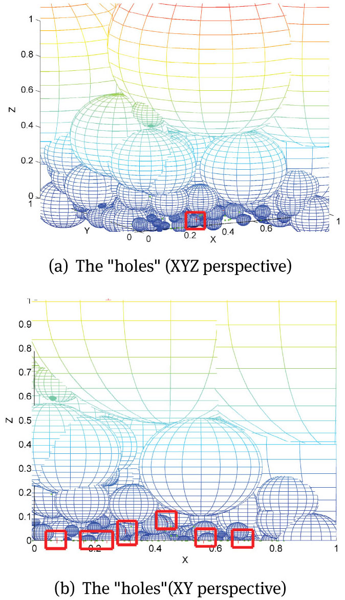
The “holes"
The traditional real negative selection algorithm trains detectors by only using one class samples (self samples), however the abnormal data (nonself samples) are easy to collect in the real practical application of anomaly detection. Similar to “vaccination” in medicine, RNSAP trains the detectors with feature preference by analyzing the “known nonself” samples. Assuming nsi is a known nonself sample, RNSAP will use the nsi to test the current mature detector set. If nsi has been covered by one of the mature detectors, it means current detectors can recognize this abnormal data. Conversely, if nsi is not covered by any mature detectors, it means the nsi falls into the hole and this hole might cause the “False negative”. In that case, RNSAP will set the feature vector of nsi as the central vector and calculate the radius to generate detector with preference. Fig. 6(a) and Fig. 6(b)(Haberman's Survival dataset) show the final performance, after combating the conventional detectors, detectors with spatial preference and detector with feature preference. Table 3 shows the algorithm of training detectors with feature preference:

The final performance of RNSAP
The algorithm of training detectors with feature preference
|
4 Experiment and discussion
4.1 Experiment setup
The V-detector algorithm is the latest version of RNSA and has shown excellent classification performance in previous work [14, 15]. In this section the comparison of V-detector and RNSAP is carried out on a 3-dimension dataset (Haberman's Survival) and 41-dimension dataset (KDD CUP99) which are widely used for testing anomaly detection system. The experiments were repeated 100 times on each dataset and the average value were adopted.
(1) Dataset
Haberman's Survival dataset contains cases from study conducted on the survival of patients who had undergone surgery for breast cancer. This dataset contains 306 records, each records contains 3 continuous fields and 1 class label [16].
KDD CUP99 dataset is consists of real world network traffic data, where each record contains 38 continuous and 3 symbolic fields and 1 class label. The complete KDD CUP99 dataset contains 3925650 abnormal sample (80.14%) and 972780 normal sample (19.86%), where the abnormal sample are partitioned in 4 categories: DOS(about 98.92%), probing(about 1.05%), U2R(about 0.0013%),R2L(about 0.0286%) [17].
(2) Measurement criterion
This paper adopted detection rate (DR), false alarm rate (FA), amount of detectors (M), training time (Ttrain) and testing time (Ttest) to measure the performance of the algorithm. The DR and FA calculate as follows:
In Eq. 10 and 11, if the anomalous sample is classified as the nonself, it is counted as a true positive (TP), if it is classified as the self, it is counted as a false negative (FN); if the normal sample is classified as the self, it is counted as a true negative (TN), if it is classified as the nonself, it is counted as a false positive (FP).
(3) The levels of RNSAP
The complete RNSAP would train three kinds of detectors: 1) The detectors with spatial preference: these detectors are trained by using the subspace information of training samples, so that could cover the subspace more effectively; 2) The detectors with feature preference: these detectors are trained by “known nonself samples”, it useful to eliminate the holes; 3) the conventional detectors: these detectors are trained randomly without any other information. In order to show the performance of the RNSAP in detail, according the training process the algorithm is divided into 3 levels:
RNSAP-1: using redundancy (R) as the algorithm termination threshold, only training the convention detectors.
RNSAP-2: using redundancy (R) as the algorithm termination threshold, training the convention detectors and the detectors with spatial preference.
RNSAP-3(complete RNSAP): using redundancy (R) as the algorithm termination threshold, training 3 kinds of detectors.
4.2 Parameters setting
(1) The radius of self sample (rs)
The rs is an important parameter in any negative selection algorithm, the smaller rs could cause false positive results while the larger rs could cause the false negative results. Many previous works have been studied rs in detail [7][15][18], so in this work it is not discussed. According to Eq. 12 this paper calculated the minimum distant (dmin) between self sample and nonself sample on Haberman's Survival Data Set and KDDCUP99. After being normalized, the dmin = 0.018 in Haberman's Survival Data Set, and dmin = 0.0056 in KDD CUP99. To equilibrate the false positive and false negative, in the following experiments the rs =0.01 on the Haberman's Survival Data Set dataset, and rs=0.003 on KDD CUP99 dataset.
In Eq. 12, i∈[1,size of selfset], j∈[1,size of nonselfset], dis(si, nsj)represents the Euclid distance between self si and nonself nsj).
(2) The “Redundant-Judgment Zone” parameter (Rc)
As discussed in section 3.1, the Rc determines the size of “Redundant-Judgment Zone”. Under the same experimental condition, the smaller Rc means the algorithm could generate more detectors, while the larger Rc indicates fewer detectors. Fig. 7 shows the influence of Rc on RNSAP-1 in 3-dimensional feature space (Haberman's Survival dataset), while Fig. 8 shows the influence in 41-dimension feature space (KDDCUP99 dataset). In these experiment the redundancy (R) is set from 0.2 to 1 step by 0.2 and other experiment setting as shown in Table 4.
the experiment setting of Rc
| Dataset | Training set | Testing set | rs |
|---|---|---|---|
| Haberman's Survival | 100%normal | 50%anomalous | 0.01 |
| KDDCUP99 | 50% normal | 50%anomalous | 0.003 |
As shown in Fig. 7 (experiment on 3D dataset), under the same redundancy (R), for Rc from 0.9 to 0.75, the number of detectors increase about 200%(Fig. 7(a)). When R>=0.6 and Rc <=0.8, The increasing detectors improve the DR only less than about 7% (Fig. 7(b)), but improve the training time by more than 100% (Fig. 7(c)). The Fig. 8 (experiment on 41D dataset) reflects the similar situation, when R>=0.6 and Rc <=0.62, the number of detectors increase 300% (Fig. 8(a)). DR increase only less than 5% (Fig. 8(b)), while the training time increases more than 150% (Fig. 8(c)). Therefore, in order to account for algorithm performance and training cost, in following experiment Rc=0.8 on the Haberman's Survival Data Set dataset, and Rc=0.62 on KDD CUP99 dataset

The influence of Rc on RNSAP-1(3D dateset)
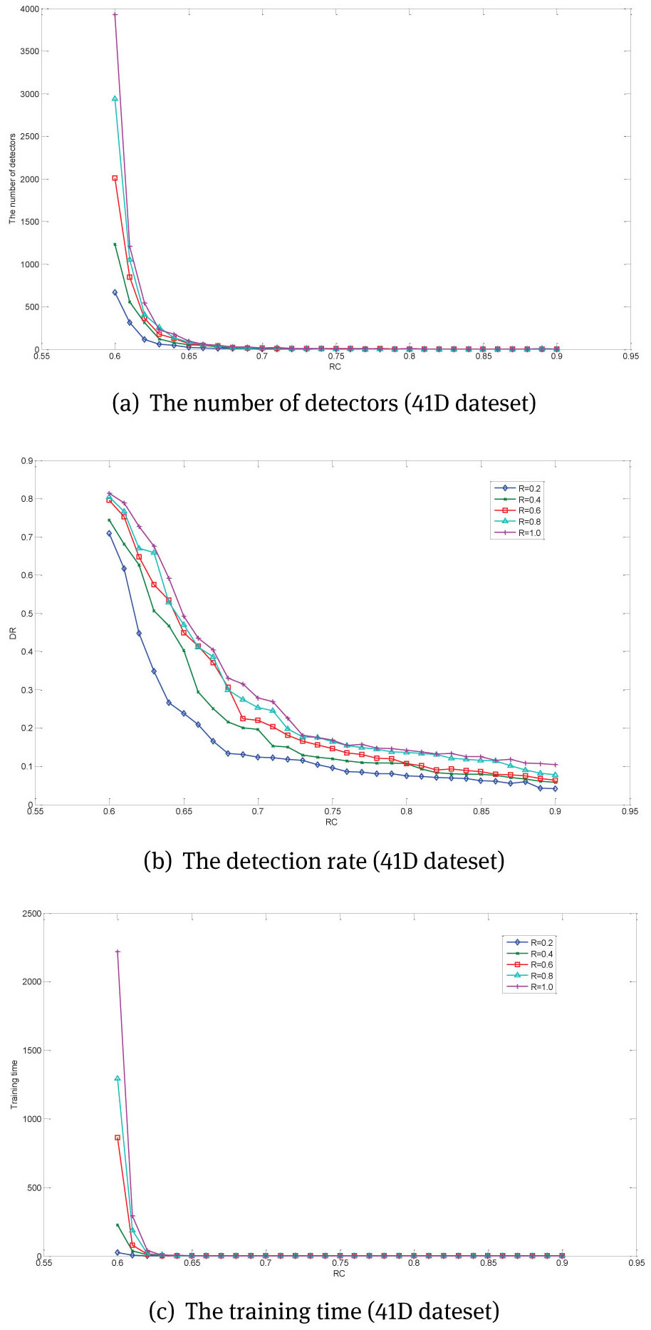
The influence of Rc on RNSAP-1(41D dateset)
In Fig. 7 and Fig. 8, when Rc=0.8 on the Haberman's Survival Data Set dataset, and Rc=0.62 on KDD CUP99 dataset, RNASP might not get the highest DR, but the training cost is acceptable. Base on the low training cost, RNASP would enhance the performance by generating the detectors with evolutionary preference (detail experimentation in 4.3 and 4.4).
4.3 Experiments on Haberman's Survival dataset
In this section, the comparison of V-detector and RNSAP is carried out on 3-dimension dataset (Haberman's Survival). The experiment is divided into 2 parts: (1) The comparison of V-detector and RNSAP-1, the experiment setting is shown in Table 5. The experiment result is shown in Table 6 and Table 7; (2)The comparison of RNSAP-1, RNSAP-2 and RNSAP-3, the experiment setting is shown in Table 8 and the experiment result is shown in Fig. 9. In these tables and figures c0 is the estimated coverage, R is the redundancy, DR is Detection rate, NOD is number of detectors, Ttrain is training time and Ttest is the testing time.
Experiment setting of V-detector and RNSAP-1 on Haberman's Survival dataset
| Algorithm | Training set | Testing set | rs |
|---|---|---|---|
| V-detector | 100%normal | randomly 50%anomalous | 0.01 |
| RNSAP-1 | 100% normal | randomly 50%anomalous | 0.01 |
The performance of V-detector
| c0 | DR | NOD | Ttrain | Ttest |
|---|---|---|---|---|
| 0.8 | 12.08% | 24 | 0.03 | 0.018 |
| 0.85 | 14.17% | 37 | 0.04 | 0.0285 |
| 0.9 | 19.16% | 61 | 0.08 | 0.044 |
| 0.92 | 23.75% | 113 | 0.17 | 0.079 |
| 0.95 | 34.58% | 126 | 0.19 | 0.087 |
| 0.99 | 62.08% | 1055 | 7.55 | 0.812 |
| 0.992 | 58.33% | 1341 | 9.52 | 0.914 |
| 0.995 | 69.92% | 2308 | 27.51 | 1.431 |
| 0.997 | 77.92% | 3746 | 72.11 | 2.388 |
| 0.999 | 84.58% | 14328 | 1054.13 | 8.768 |
The performance of RNSAP-1
| R | DR | NOD | Ttrain | Ttest |
|---|---|---|---|---|
| 0.1 | 48.75% | 195 | 3.58 | 0.15 |
| 0.2 | 58.33% | 379 | 12.76 | 0.37 |
| 0.3 | 64.58% | 441 | 19.31 | 0.52 |
| 0.4 | 71.25% | 589 | 36.84 | 0.61 |
| 0.5 | 82.08% | 798 | 77.43 | 0.72 |
| 0.6 | 83.33% | 927 | 97.91 | 0.84 |
| 0.7 | 83.75% | 991 | 146.24 | 0.92 |
| 0.8 | 85.42% | 1093 | 173.32 | 0.97 |
| 0.9 | 88.92% | 1134 | 231.22 | 1.08 |
| 1.0 | 89.25% | 1178 | 242.35 | 1.16 |
Both V-detector and RNSAP-1 generate detectors randomly, however RNSAP-1 uses the redundancy (R) instead of the Estimate Coverage (c0) as the algorithm termination condition. In Ttable 6 (V-detector), when (c0) grew up from 0.997 to 0.999, DR only increased by approximately 6.6%. By contrast, NOD (number of detectors) increased approximately 400%. Ttrain increased approximately 1000% and Ttest increased approximately 300%. This is resultant from highly redundant detectors in feature space. Theses redundant detectors overlapped with each other can hardly improve the detector rate, but wasted lots of training resource. Comparing Table 6 (V-detector) to Table 7 (RNSAP-1), when DR got 84.58% (c0=0.999), V-detector generated 14328 detectors, and took 1054 seconds; obtained a similar DR 85.42%, RNSAP-1 only generate 1093 detectors and took 209 seconds. RNSAP-1 got the highest DR 89.25% only generate 1178 detectors, and took 274 seconds. The experiment result revealed that by adopting redundancy testing, RNSAP-1 removed a plenty of redundant detectors and enhanced the quality of conventional detectors, so that RNSAP-1 achieved a higher detection rate with less detectors and training time.
Experiment setting of 3 levels RNSAP on Haberman's Survival dataset
| Algorithm | Training set | Testing set | rs |
|---|---|---|---|
| RNSAP-1 | 100%normal | 50%anomalous | 0.01 |
| RNSAP-2 | 100%normal | 50%anomalous | 0.01 |
| RNSAP-3 | 100%normal,30%anomalous | 70%anomalous | 0.01 |
As presented in section 4.2, the RNSAP-1 only generates conventional detectors, RNSAP-2 generates both conventional detectors and detectors with spatial preference, and the RNSAP-3(complete RNSAP) generates 3 kinds of detectors. As shown in Fig. 9(a), by training the detectors with spatial preference and feature preference, RNSAP-3 improved the lowest detection rate from 48.75% to 71.23%, and improved the highest detection from 89.25% to 96.72%. In Fig. 9(b) and Fig. 9(c), for training the detectors with evolutionary preference the number of detectors grew, however the training time increased less than 15%. It is worth mentioning in Fig. 9, the detectors with feature preference were rarely generated when R reached 0.5, this because in 3-dimensional space the conventional detectors and the detectors spatial preference had covered nearly all of the feature space.
At last, compare Table 6 to Fig. 9, for V-detector, when DR was at 84.58%, 14328 detectors were needed at a cost of 2368 seconds; RNSAP-3(complete RNSAP) improved DR to 96.72 % (R=1), and only needed 2112 detectors at a cost of 274.47 seconds.

The comparison of 3 levels RNSAP
4.4 Experiments on KDD CUP99 dataset
In this section, a contrast experiment is carried on the 41-dimension dataset (KDDCUP-99). The same as in section 4.3, firstly a comparison of V-detector and RNSAP-1 (experiment setting is shown in Table 9) is given in Table 10–Table 12. Secondly, a comparison of RNSAP-1, RNSAP-2 and RNSAP-3(the experiment setting as shown in Table 13) is shown in Fig. 10. In these tables, c0 is Estimate Coverage; R is redundancy; DR is Detection rate; FR is False alarm rate; MND is The maximum number of detectors; Ttrain is training time; Ttest is testing time.
Experiment setting of 3 levels RNSAP on KDDCUP99
| Algorithm | Training set | Testing set | rs |
|---|---|---|---|
| V-detector | 50% normal | randomly 50% anomalous | 0.003 |
| RNSAP-1 | 50% normal | randomly 50% anomalous | 0.003 |
The performance of V-detector (co)
| c0 | DR | FR | NOD | Ttrain | Ttest |
|---|---|---|---|---|---|
| 0.8 | 5.71% | 0.056% | 2 | 0.039 | 0.078 |
| 0.85 | 6.49% | 0.068% | 2 | 0.042 | 0.085 |
| 0.9 | 7.92% | 0.046% | 2 | 0.040 | 0.079 |
| 0.92 | 8.32% | 0.062% | 2 | 0.044 | 0.089 |
| 0.95 | 8.96% | 0.024% | 2 | 0.047 | 0.083 |
| 0.99 | 9.72% | 0.038% | 2 | 0.049 | 0.092 |
| 0.992 | 9.82% | 0.041% | 3 | 0.052 | 0.113 |
| 0.995 | 9.93% | 0.047% | 3 | 0.056 | 0.093 |
| 0.997 | 10.51% | 0.052% | 3 | 0.057 | 0.108 |
| 0.999 | 12.07% | 0.064% | 4 | 0.088 | 0.113 |
The performance of V-detector (MND)
| MND | DR | FR | Ttrain | Ttest |
|---|---|---|---|---|
| 300 | 52.12% | 0.41% | 4.92 | 1.86 |
| 800 | 61.03% | 0.62% | 13.81 | 5.15 |
| 1500 | 66.32% | 0.79% | 24.47 | 11.90 |
| 3000 | 63.91% | 0.94% | 49.45 | 19.41 |
| 5500 | 68.40% | 1.03% | 94.83 | 37.60 |
| 10000 | 73.88% | 1.24% | 207.22 | 53.21 |
| 20000 | 74.42% | 1.41% | 452.76 | 84.53 |
| 30000 | 75.49% | 1.45% | 805.68 | 171.96 |
| 40000 | 76.53% | 1.57% | 1308.16 | 336.68 |
| 50000 | 76.82% | 1.59% | 1814.13 | 575.38 |
The performance of NASP-1
| R | DR | FR | NOD | Ttrain | Ttest |
|---|---|---|---|---|---|
| 0.1 | 63.91% | 0.66% | 264 | 10.63 | 2.914 |
| 0.2 | 64.62% | 0.73% | 313 | 11.25 | 3.231 |
| 0.3 | 66.52% | 0.81% | 321 | 13.93 | 3.337 |
| 0.4 | 71.24% | 1.09% | 402 | 19.32 | 3.466 |
| 0.5 | 71.93% | 1.18% | 424 | 21.93 | 3.486 |
| 0.6 | 73.69% | 1.17% | 474 | 27.20 | 3.626 |
| 0.7 | 75.18% | 1.29% | 492 | 33.84 | 3.748 |
| 0.8 | 75.51% | 1.43% | 517 | 38.27 | 3.799 |
| 0.9 | 76.63% | 1.61% | 536 | 41.95 | 3.887 |
| 1.0 | 76.91% | 1.77% | 585 | 46.11 | 3.953 |
Experiment setting of 3 levels RNSAP on KDDCUP99
| Algorithm | Training set | Testing set | rs |
|---|---|---|---|
| RNSAP-1 | 100%normal | 50%anomalous | 0.003 |
| RNSAP-2 | 100%normal | 50%anomalous | 0.003 |
| RNSAP-3 | 100%normal,30%anomalous | 70%anomalous | 0.003 |
In Table 10, by using the estimated coverage (c0) as the termination condition, V-detector can barely generate detectors, it leads to the poor performance. For example, when c0=99.9% only 4 detectors were generated. Although the number of detectors is scarce, the mean radius of theses detectors reached 3. According to the volume of hyper-sphere Eq. 13, when dimension n=41 and the hypersphere radius r=3, the volume (V) of single 41-dimensional detector is approximately 5*1011. In contrast, the feature space was a 41-dimension hypercube with total volume=1, so the single detector had covered almost whole feature space (central area). In that situation, the “point estimate” Eq.2 would satisfy quickly. It caused to the algorithm be terminated unexpected when the detectors were not enough. More importantly, as discussed in section 3.1, in high-dimension space a part of the samples would distribute in the subspace (edge area), the few mature 41-dimensional conventional detectors hardly cover these samples.
In Table 11, by using the Maximum Number of Detectors (MND) as the termination condition, V-detector can get DR=76.82%. It reflected that if there were enough detectors, V-detector still can recognize the training samples in high-dimension space. But the disadvantage was obvious by using maximum number of detectors (MND) as the termination threshold: firstly, the MND is difficult to accurately forecast; second, with the detectors overlapping each other in feature space, it cannot guarantee that the mature detectors set can cover enough nonself space when MND reached the threshold; lastly, plenty of redundant detectors cannot improve the detector rate but wasted the calculation resource. In Table 11 after MND reached 10000, the DR fluctuated around 74%. Specially, compared to MND = 50000, when MND= 10000 the detectors increased about 500%, Ttrain increased about 900%, but the detection rate increased less than 3%.
In Table 12, RNSAP-1 adopted the redundancy(R) as the terminate condition to generate 41-dimension conventional detectors. Compared to Table 10 (V-detector using c0), RNSAP-1 can improve the DR to 76.91% by generating enough detectors. Compared to Table 11 (V-detector using MND), RNSAP-1 can achieve the similar performance with less detectors and training time. In Table 11, when DR=76.82% and FR=1.59%, V-detector generated 50000 detectors and cost 1814 seconds. In Table 12, when DR=76.91% and FR=1.77% (R=1), RNSAP-1 only need 585 detectors and 46.11 seconds.
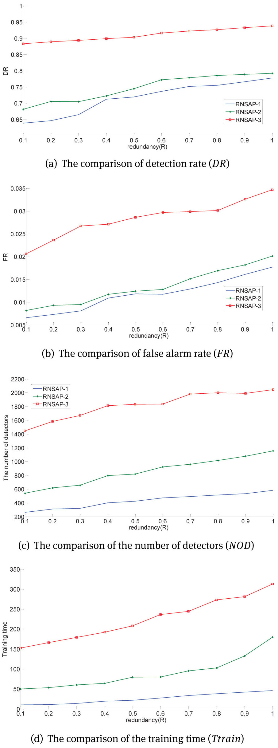
The comparison of the 3 levels RNSAP shown in Fig. 10. The same as the low-dimension experiment, by training the detectors with spatial preference and feature preference, RNSAP-3 can improve the DR with similar FR and acceptable training cost. In Fig. 10(a), RNSAP-3 improved the lowest detection rate from 63.91% to 86.84%, and improved the highest detection from 76.91% to 91.24%. Although the DR had been improved more than 15%, the FR only had been raised less than 0.15% (Fig. 10(b)). In Fig. 10(c), on each redundancy(R) about more than 1000 detectors with evolutionary preference were generated, however the training time increased less than 300 seconds.
At last, compare Table 10 to Fig. 10, if V-detector adopted c0 as the termination condition, the DR can only achieve about 12%, the shorter training time was due to almost no detectors being generated; V-detector adopted MND as termination condition, when DR=76.82% and FA=1.59%, 50000 detectors need generated and cost 1814 seconds; RNSAP-3(complete RNSAP) improved DR to 91.24% (R=1), need only 2086 detectors and cost 313.46 seconds.
The comparison of the 3 levels RNSAP
5 Conclusion
The negative selection algorithm has caught the attention of researchers due to its unique property of anomaly detection. However, the problem about how to generate effective detectors in high-dimensional space has not been solved properly in previous research work and artificial immune applications. This paper introduces a real negative selection algorithm with evolutionary preference (RNSAP). By using redundant as the algorithm termination threshold and generating detectors with evolutionary preference, RNSAP can cover the nonself space more effectively in high-dimensional space. Theoretical analysis and experimental results show that RNSAP has better time efficiency and detector quality compared with classical negative selection algorithms, and it can be competent in the task of anomaly detection for both low-dimensional space and high-dimensional space.
Acknowledgement
This work has been supported by the National Key Research and Development Program of China under Grant No. 2016YFB0800604 and No. 2016YFB0800605, National Natural Science Foundation of China under Grant no.61173159, the National Natural Science Foundation of China under Grant no.614020308.
References
[1] Forrest S., Perelson A.S., Lawrence A., Cherukuri R., Self-Nonself Discrimination in a Computer, Proceedings of IEEE Computer Society Symposium on Research in Security and Privacy, (16-18 May 1994, DC, USA), DC, 1994, 202-212.10.1109/RISP.1994.296580Search in Google Scholar
[2] Laurentys C.A., Ronacher G., Palhares R.M., Caminhas W.M., Design of an Artificial Immune System for fault detection: A Negative Selection Approach, Expert Syst. App., 2010, 37, 5507-5513.10.1016/j.eswa.2010.02.004Search in Google Scholar
[3] Jinquan Z., Zhiguang Q., Weiwen T., Anomaly Detection Using a Novel Negative Selection Algorithm, J. Comput. Theor. Nanosci., 2013, 10, 2831-2835.10.1166/jctn.2013.3286Search in Google Scholar
[4] Idris I., Selamat A., Omatu S., Hybrid email spam detection model with negative selection algorithm and differential evolution, Eng. Appl. Artif. Intell., 2014, 28, 97-110.10.1016/j.engappai.2013.12.001Search in Google Scholar
[5] Hualong W., Bo Z., Overview of current techniques in remote data auditing, Appl. Math. Nonlinear Sci., 2016, 145-158.10.21042/AMNS.2016.1.00011Search in Google Scholar
[6] Gonzalez F., Dasgupta D., Nio L.F., A Randomized Real-Valued Negative Selection Algorithm, Lect. Notes. Comput. Sc., 2003, 2787, 261-272.10.1007/978-3-540-45192-1_25Search in Google Scholar
[7] Ji Z., Dasgupta D., Real-Valued Negative Selection Algorithm with Variable-Sized Detectors, Lect. Notes. Comput. Sc, 2004, 3102, 287-298.10.1007/978-3-540-24854-5_30Search in Google Scholar
[8] Maoguo G., Jian Z., Jingjing M., Licheng J., An efficient negative selection algorithm with further training for anomaly detection, Knowl-Based. Syst., 2012, 30, 185-191.10.1016/j.knosys.2012.01.004Search in Google Scholar
[9] Wen C., Tao L., XiaoJie L., Bing Z., A negative selection algorithm based on hierarchical clustering of self set, Adv. Mater. Res., 2013, 56, 1-13.10.1007/s11432-011-4323-7Search in Google Scholar
[10] Poggiolini M., Engelbrecht A., Application of the featuredetection rule to the Negative Selection Algorithm, Expert Syst. App., 2013, 40, 3001-3014.10.1016/j.eswa.2012.12.016Search in Google Scholar
[11] Fernandez M., A survey on fractal dimension for fractal structures, Appl. Math. Nonlinear Sci., 2016, 1, 437-472.10.21042/AMNS.2016.2.00037Search in Google Scholar
[12] Perelson A.S., Weisbuch G., Immunology for physicists, Rev. Mod. Phys., 1997, 69, 1219-1267.10.1103/RevModPhys.69.1219Search in Google Scholar
[13] Yang Z., Meyerhermann M., George L.A., Figge M.T., Khan M., Goodall M., et al., Germinal center B cells govern their own fate via antibody feedback, J. Exp. Med., 2013, 210, 457-464.10.1084/jem.20120150Search in Google Scholar PubMed PubMed Central
[14] Ji Z., Dasgupta D., Estimating the detector coverage in a negative selection algorithm, Proceedings of Genetic and Evolutionary Computation Conference (25-29 June 2005, Washington DC, USA), New York, 2005, 281-289, 10.1145/1068009.1068056.Search in Google Scholar
[15] Ji Z., Dasgupta D., V-detector: An efficient negative selection algorithm with “probably adequate” detector coverage, Inform. Sciences, 2009, 179, 1390-1406.10.1016/j.ins.2008.12.015Search in Google Scholar
[16] Haberman datasets. http://archive.ics.uci.edu/ml/datasets/Haberman.Search in Google Scholar
[17] Kddcup datasets. http://archive.ics.uci.edu/ml/datasets/KDD+Cup+1999+Data.Search in Google Scholar
[18] Stibor T., Timmis J., Eckert C., On the Use of Hyperspheres in Artificial Immune Systems as Antibody Recognition Regions, Proceedings of International Conference on Artificial Immune Systems (4-6 September 2006, Portugal), Portugal, 2006, 215-228.10.1007/11823940_17Search in Google Scholar
© 2017 Tao Yang et al.
This work is licensed under the Creative Commons Attribution-NonCommercial-NoDerivatives 3.0 License.
Articles in the same Issue
- Regular Articles
- Analysis of a New Fractional Model for Damped Bergers’ Equation
- Regular Articles
- Optimal homotopy perturbation method for nonlinear differential equations governing MHD Jeffery-Hamel flow with heat transfer problem
- Regular Articles
- Semi- analytic numerical method for solution of time-space fractional heat and wave type equations with variable coefficients
- Regular Articles
- Investigation of a curve using Frenet frame in the lightlike cone
- Regular Articles
- Construction of complex networks from time series based on the cross correlation interval
- Regular Articles
- Nonlinear Schrödinger approach to European option pricing
- Regular Articles
- A modified cubic B-spline differential quadrature method for three-dimensional non-linear diffusion equations
- Regular Articles
- A new miniaturized negative-index meta-atom for tri-band applications
- Regular Articles
- Seismic stability of the survey areas of potential sites for the deep geological repository of the spent nuclear fuel
- Regular Articles
- Distributed containment control of heterogeneous fractional-order multi-agent systems with communication delays
- Regular Articles
- Sensitivity analysis and economic optimization studies of inverted five-spot gas cycling in gas condensate reservoir
- Regular Articles
- Quantum mechanics with geometric constraints of Friedmann type
- Regular Articles
- Modeling and Simulation for an 8 kW Three-Phase Grid-Connected Photo-Voltaic Power System
- Regular Articles
- Application of the optimal homotopy asymptotic method to nonlinear Bingham fluid dampers
- Regular Articles
- Analysis of Drude model using fractional derivatives without singular kernels
- Regular Articles
- An unsteady MHD Maxwell nanofluid flow with convective boundary conditions using spectral local linearization method
- Regular Articles
- New analytical solutions for conformable fractional PDEs arising in mathematical physics by exp-function method
- Regular Articles
- Quantum mechanical calculation of electron spin
- Regular Articles
- CO2 capture by polymeric membranes composed of hyper-branched polymers with dense poly(oxyethylene) comb and poly(amidoamine)
- Regular Articles
- Chain on a cone
- Regular Articles
- Multi-task feature learning by using trace norm regularization
- Regular Articles
- Superluminal tunneling of a relativistic half-integer spin particle through a potential barrier
- Regular Articles
- Neutrosophic triplet normed space
- Regular Articles
- Lie algebraic discussion for affinity based information diffusion in social networks
- Regular Articles
- Radiation dose and cancer risk estimates in helical CT for pulmonary tuberculosis infections
- Regular Articles
- A comparison study of steady-state vibrations with single fractional-order and distributed-order derivatives
- Regular Articles
- Some new remarks on MHD Jeffery-Hamel fluid flow problem
- Regular Articles
- Numerical investigation of magnetohydrodynamic slip flow of power-law nanofluid with temperature dependent viscosity and thermal conductivity over a permeable surface
- Regular Articles
- Charge conservation in a gravitational field in the scalar ether theory
- Regular Articles
- Measurement problem and local hidden variables with entangled photons
- Regular Articles
- Compression of hyper-spectral images using an accelerated nonnegative tensor decomposition
- Regular Articles
- Fabrication and application of coaxial polyvinyl alcohol/chitosan nanofiber membranes
- Regular Articles
- Calculating degree-based topological indices of dominating David derived networks
- Regular Articles
- The structure and conductivity of polyelectrolyte based on MEH-PPV and potassium iodide (KI) for dye-sensitized solar cells
- Regular Articles
- Chiral symmetry restoration and the critical end point in QCD
- Regular Articles
- Numerical solution for fractional Bratu’s initial value problem
- Regular Articles
- Structure and optical properties of TiO2 thin films deposited by ALD method
- Regular Articles
- Quadruple multi-wavelength conversion for access network scalability based on cross-phase modulation in an SOA-MZI
- Regular Articles
- Application of ANNs approach for wave-like and heat-like equations
- Special issue on Nonlinear Dynamics in General and Dynamical Systems in particular
- Study on node importance evaluation of the high-speed passenger traffic complex network based on the Structural Hole Theory
- Special issue on Nonlinear Dynamics in General and Dynamical Systems in particular
- A mathematical/physics model to measure the role of information and communication technology in some economies: the Chinese case
- Special issue on Nonlinear Dynamics in General and Dynamical Systems in particular
- Numerical modeling of the thermoelectric cooler with a complementary equation for heat circulation in air gaps
- Special issue on Nonlinear Dynamics in General and Dynamical Systems in particular
- On the libration collinear points in the restricted three – body problem
- Special issue on Nonlinear Dynamics in General and Dynamical Systems in particular
- Research on Critical Nodes Algorithm in Social Complex Networks
- Special issue on Nonlinear Dynamics in General and Dynamical Systems in particular
- A simulation based research on chance constrained programming in robust facility location problem
- Special issue on Nonlinear Dynamics in General and Dynamical Systems in particular
- A mathematical/physics carbon emission reduction strategy for building supply chain network based on carbon tax policy
- Special issue on Nonlinear Dynamics in General and Dynamical Systems in particular
- Mathematical analysis of the impact mechanism of information platform on agro-product supply chain and agro-product competitiveness
- Special issue on Nonlinear Dynamics in General and Dynamical Systems in particular
- A real negative selection algorithm with evolutionary preference for anomaly detection
- Special issue on Nonlinear Dynamics in General and Dynamical Systems in particular
- A privacy-preserving parallel and homomorphic encryption scheme
- Special issue on Nonlinear Dynamics in General and Dynamical Systems in particular
- Random walk-based similarity measure method for patterns in complex object
- Special issue on Nonlinear Dynamics in General and Dynamical Systems in particular
- A Mathematical Study of Accessibility and Cohesion Degree in a High-Speed Rail Station Connected to an Urban Bus Transport Network
- Special issue on Nonlinear Dynamics in General and Dynamical Systems in particular
- Design and Simulation of the Integrated Navigation System based on Extended Kalman Filter
- Special issue on Nonlinear Dynamics in General and Dynamical Systems in particular
- Oil exploration oriented multi-sensor image fusion algorithm
- Special issue on Nonlinear Dynamics in General and Dynamical Systems in particular
- Analysis of Product Distribution Strategy in Digital Publishing Industry Based on Game-Theory
- Special issue on Nonlinear Dynamics in General and Dynamical Systems in particular
- Expanded Study on the accumulation effect of tourism under the constraint of structure
- Special issue on Nonlinear Dynamics in General and Dynamical Systems in particular
- Unstructured P2P Network Load Balance Strategy Based on Multilevel Partitioning of Hypergraph
- Special issue on Nonlinear Dynamics in General and Dynamical Systems in particular
- Research on the method of information system risk state estimation based on clustering particle filter
- Special issue on Nonlinear Dynamics in General and Dynamical Systems in particular
- Demand forecasting and information platform in tourism
- Special issue on Nonlinear Dynamics in General and Dynamical Systems in particular
- Physical-chemical properties studying of molecular structures via topological index calculating
- Special issue on Nonlinear Dynamics in General and Dynamical Systems in particular
- Local kernel nonparametric discriminant analysis for adaptive extraction of complex structures
- Special issue on Nonlinear Dynamics in General and Dynamical Systems in particular
- City traffic flow breakdown prediction based on fuzzy rough set
- Special issue on Nonlinear Dynamics in General and Dynamical Systems in particular
- Conservation laws for a strongly damped wave equation
- Special issue on Nonlinear Dynamics in General and Dynamical Systems in particular
- Blending type approximation by Stancu-Kantorovich operators based on Pólya-Eggenberger distribution
- Special issue on Nonlinear Dynamics in General and Dynamical Systems in particular
- Computing the Ediz eccentric connectivity index of discrete dynamic structures
- Special issue on Nonlinear Dynamics in General and Dynamical Systems in particular
- A discrete epidemic model for bovine Babesiosis disease and tick populations
- Special issue on Nonlinear Dynamics in General and Dynamical Systems in particular
- Study on maintaining formations during satellite formation flying based on SDRE and LQR
- Special issue on Nonlinear Dynamics in General and Dynamical Systems in particular
- Relationship between solitary pulmonary nodule lung cancer and CT image features based on gradual clustering
- Special issue on Nonlinear Dynamics in General and Dynamical Systems in particular
- A novel fast target tracking method for UAV aerial image
- Special issue on Nonlinear Dynamics in General and Dynamical Systems in particular
- Fuzzy comprehensive evaluation model of interuniversity collaborative learning based on network
- Special issue on Nonlinear Dynamics in General and Dynamical Systems in particular
- Conservation laws, classical symmetries and exact solutions of the generalized KdV-Burgers-Kuramoto equation
- Special issue on Nonlinear Dynamics in General and Dynamical Systems in particular
- After notes on self-similarity exponent for fractal structures
- Special issue on Nonlinear Dynamics in General and Dynamical Systems in particular
- Excitation probability and effective temperature in the stationary regime of conductivity for Coulomb Glasses
- Special issue on Nonlinear Dynamics in General and Dynamical Systems in particular
- Comparisons of feature extraction algorithm based on unmanned aerial vehicle image
- Special issue on Nonlinear Dynamics in General and Dynamical Systems in particular
- Research on identification method of heavy vehicle rollover based on hidden Markov model
- Special issue on Nonlinear Dynamics in General and Dynamical Systems in particular
- Classifying BCI signals from novice users with extreme learning machine
- Special issue on Nonlinear Dynamics in General and Dynamical Systems in particular
- Topics on data transmission problem in software definition network
- Special issue on Nonlinear Dynamics in General and Dynamical Systems in particular
- Statistical inferences with jointly type-II censored samples from two Pareto distributions
- Special issue on Nonlinear Dynamics in General and Dynamical Systems in particular
- Estimation for coefficient of variation of an extension of the exponential distribution under type-II censoring scheme
- Special issue on Nonlinear Dynamics in General and Dynamical Systems in particular
- Analysis on trust influencing factors and trust model from multiple perspectives of online Auction
- Special Issue on Advances on Modelling of Flowing and Transport in Porous Media
- Coupling of two-phase flow in fractured-vuggy reservoir with filling medium
- Special Issue on Advances on Modelling of Flowing and Transport in Porous Media
- Production decline type curves analysis of a finite conductivity fractured well in coalbed methane reservoirs
- Special Issue on Advances on Modelling of Flowing and Transport in Porous Media
- Flow Characteristic and Heat Transfer for Non-Newtonian Nanofluid in Rectangular Microchannels with Teardrop Dimples/Protrusions
- Special Issue on Advances on Modelling of Flowing and Transport in Porous Media
- The size prediction of potential inclusions embedded in the sub-surface of fused silica by damage morphology
- Special Issue on Advances on Modelling of Flowing and Transport in Porous Media
- Research on carbonate reservoir interwell connectivity based on a modified diffusivity filter model
- Special Issue on Advances on Modelling of Flowing and Transport in Porous Media
- The method of the spatial locating of macroscopic throats based-on the inversion of dynamic interwell connectivity
- Special Issue on Advances on Modelling of Flowing and Transport in Porous Media
- Unsteady mixed convection flow through a permeable stretching flat surface with partial slip effects through MHD nanofluid using spectral relaxation method
- Special Issue on Advances on Modelling of Flowing and Transport in Porous Media
- A volumetric ablation model of EPDM considering complex physicochemical process in porous structure of char layer
- Special Issue on Advances on Modelling of Flowing and Transport in Porous Media
- Numerical simulation on ferrofluid flow in fractured porous media based on discrete-fracture model
- Special Issue on Advances on Modelling of Flowing and Transport in Porous Media
- Macroscopic lattice Boltzmann model for heat and moisture transfer process with phase transformation in unsaturated porous media during freezing process
- Special Issue on Advances on Modelling of Flowing and Transport in Porous Media
- Modelling of intermittent microwave convective drying: parameter sensitivity
- Special Issue on Advances on Modelling of Flowing and Transport in Porous Media
- Simulating gas-water relative permeabilities for nanoscale porous media with interfacial effects
- Special Issue on Advances on Modelling of Flowing and Transport in Porous Media
- Simulation of counter-current imbibition in water-wet fractured reservoirs based on discrete-fracture model
- Special Issue on Advances on Modelling of Flowing and Transport in Porous Media
- Investigation effect of wettability and heterogeneity in water flooding and on microscopic residual oil distribution in tight sandstone cores with NMR technique
- Special Issue on Advances on Modelling of Flowing and Transport in Porous Media
- Analytical modeling of coupled flow and geomechanics for vertical fractured well in tight gas reservoirs
- Special Issue on Ever-New "Loopholes" in Bell’s Argument and Experimental Tests
- Special Issue: Ever New "Loopholes" in Bell’s Argument and Experimental Tests
- Special Issue on Ever-New "Loopholes" in Bell’s Argument and Experimental Tests
- The ultimate loophole in Bell’s theorem: The inequality is identically satisfied by data sets composed of ±1′s assuming merely that they exist
- Special Issue on Ever-New "Loopholes" in Bell’s Argument and Experimental Tests
- Erratum to: The ultimate loophole in Bell’s theorem: The inequality is identically satisfied by data sets composed of ±1′s assuming merely that they exist
- Special Issue on Ever-New "Loopholes" in Bell’s Argument and Experimental Tests
- Rhetoric, logic, and experiment in the quantum nonlocality debate
- Special Issue on Ever-New "Loopholes" in Bell’s Argument and Experimental Tests
- What If Quantum Theory Violates All Mathematics?
- Special Issue on Ever-New "Loopholes" in Bell’s Argument and Experimental Tests
- Relativity, anomalies and objectivity loophole in recent tests of local realism
- Special Issue on Ever-New "Loopholes" in Bell’s Argument and Experimental Tests
- The photon identification loophole in EPRB experiments: computer models with single-wing selection
- Special Issue on Ever-New "Loopholes" in Bell’s Argument and Experimental Tests
- Bohr against Bell: complementarity versus nonlocality
- Special Issue on Ever-New "Loopholes" in Bell’s Argument and Experimental Tests
- Is Einsteinian no-signalling violated in Bell tests?
- Special Issue on Ever-New "Loopholes" in Bell’s Argument and Experimental Tests
- Bell’s “Theorem”: loopholes vs. conceptual flaws
- Special Issue on Ever-New "Loopholes" in Bell’s Argument and Experimental Tests
- Nonrecurrence and Bell-like inequalities
- Special Issue: The 18th International Symposium on Electromagnetic Fields in Mechatronics, Electrical and Electronic Engineering ISEF 2017
- Three-dimensional computer models of electrospinning systems
- Special Issue: The 18th International Symposium on Electromagnetic Fields in Mechatronics, Electrical and Electronic Engineering ISEF 2017
- Electric field computation and measurements in the electroporation of inhomogeneous samples
- Special Issue: The 18th International Symposium on Electromagnetic Fields in Mechatronics, Electrical and Electronic Engineering ISEF 2017
- Modelling of magnetostriction of transformer magnetic core for vibration analysis
- Special Issue: The 18th International Symposium on Electromagnetic Fields in Mechatronics, Electrical and Electronic Engineering ISEF 2017
- Comparison of the fractional power motor with cores made of various magnetic materials
- Special Issue: The 18th International Symposium on Electromagnetic Fields in Mechatronics, Electrical and Electronic Engineering ISEF 2017
- Dynamics of the line-start reluctance motor with rotor made of SMC material
- Special Issue: The 18th International Symposium on Electromagnetic Fields in Mechatronics, Electrical and Electronic Engineering ISEF 2017
- Inhomogeneous dielectrics: conformal mapping and finite-element models
- Special Issue: The 18th International Symposium on Electromagnetic Fields in Mechatronics, Electrical and Electronic Engineering ISEF 2017
- Topology optimization of induction heating model using sequential linear programming based on move limit with adaptive relaxation
- Special Issue: The 18th International Symposium on Electromagnetic Fields in Mechatronics, Electrical and Electronic Engineering ISEF 2017
- Detection of inter-turn short-circuit at start-up of induction machine based on torque analysis
- Special Issue: The 18th International Symposium on Electromagnetic Fields in Mechatronics, Electrical and Electronic Engineering ISEF 2017
- Current superimposition variable flux reluctance motor with 8 salient poles
- Special Issue: The 18th International Symposium on Electromagnetic Fields in Mechatronics, Electrical and Electronic Engineering ISEF 2017
- Modelling axial vibration in windings of power transformers
- Special Issue: The 18th International Symposium on Electromagnetic Fields in Mechatronics, Electrical and Electronic Engineering ISEF 2017
- Field analysis & eddy current losses calculation in five-phase tubular actuator
- Special Issue: The 18th International Symposium on Electromagnetic Fields in Mechatronics, Electrical and Electronic Engineering ISEF 2017
- Hybrid excited claw pole generator with skewed and non-skewed permanent magnets
- Special Issue: The 18th International Symposium on Electromagnetic Fields in Mechatronics, Electrical and Electronic Engineering ISEF 2017
- Electromagnetic phenomena analysis in brushless DC motor with speed control using PWM method
- Special Issue: The 18th International Symposium on Electromagnetic Fields in Mechatronics, Electrical and Electronic Engineering ISEF 2017
- Field-circuit analysis and measurements of a single-phase self-excited induction generator
- Special Issue: The 18th International Symposium on Electromagnetic Fields in Mechatronics, Electrical and Electronic Engineering ISEF 2017
- A comparative analysis between classical and modified approach of description of the electrical machine windings by means of T0 method
- Special Issue: The 18th International Symposium on Electromagnetic Fields in Mechatronics, Electrical and Electronic Engineering ISEF 2017
- Field-based optimal-design of an electric motor: a new sensitivity formulation
- Special Issue: The 18th International Symposium on Electromagnetic Fields in Mechatronics, Electrical and Electronic Engineering ISEF 2017
- Application of the parametric proper generalized decomposition to the frequency-dependent calculation of the impedance of an AC line with rectangular conductors
- Special Issue: The 18th International Symposium on Electromagnetic Fields in Mechatronics, Electrical and Electronic Engineering ISEF 2017
- Virtual reality as a new trend in mechanical and electrical engineering education
- Special Issue: The 18th International Symposium on Electromagnetic Fields in Mechatronics, Electrical and Electronic Engineering ISEF 2017
- Holonomicity analysis of electromechanical systems
- Special Issue: The 18th International Symposium on Electromagnetic Fields in Mechatronics, Electrical and Electronic Engineering ISEF 2017
- An accurate reactive power control study in virtual flux droop control
- Special Issue: The 18th International Symposium on Electromagnetic Fields in Mechatronics, Electrical and Electronic Engineering ISEF 2017
- Localized probability of improvement for kriging based multi-objective optimization
- Special Issue: The 18th International Symposium on Electromagnetic Fields in Mechatronics, Electrical and Electronic Engineering ISEF 2017
- Research of influence of open-winding faults on properties of brushless permanent magnets motor
- Special Issue: The 18th International Symposium on Electromagnetic Fields in Mechatronics, Electrical and Electronic Engineering ISEF 2017
- Optimal design of the rotor geometry of line-start permanent magnet synchronous motor using the bat algorithm
- Special Issue: The 18th International Symposium on Electromagnetic Fields in Mechatronics, Electrical and Electronic Engineering ISEF 2017
- Model of depositing layer on cylindrical surface produced by induction-assisted laser cladding process
- Special Issue: The 18th International Symposium on Electromagnetic Fields in Mechatronics, Electrical and Electronic Engineering ISEF 2017
- Detection of inter-turn faults in transformer winding using the capacitor discharge method
- Special Issue: The 18th International Symposium on Electromagnetic Fields in Mechatronics, Electrical and Electronic Engineering ISEF 2017
- A novel hybrid genetic algorithm for optimal design of IPM machines for electric vehicle
- Special Issue: The 18th International Symposium on Electromagnetic Fields in Mechatronics, Electrical and Electronic Engineering ISEF 2017
- Lamination effects on a 3D model of the magnetic core of power transformers
- Special Issue: The 18th International Symposium on Electromagnetic Fields in Mechatronics, Electrical and Electronic Engineering ISEF 2017
- Detection of vertical disparity in three-dimensional visualizations
- Special Issue: The 18th International Symposium on Electromagnetic Fields in Mechatronics, Electrical and Electronic Engineering ISEF 2017
- Calculations of magnetic field in dynamo sheets taking into account their texture
- Special Issue: The 18th International Symposium on Electromagnetic Fields in Mechatronics, Electrical and Electronic Engineering ISEF 2017
- 3-dimensional computer model of electrospinning multicapillary unit used for electrostatic field analysis
- Special Issue: The 18th International Symposium on Electromagnetic Fields in Mechatronics, Electrical and Electronic Engineering ISEF 2017
- Optimization of wearable microwave antenna with simplified electromagnetic model of the human body
- Special Issue: The 18th International Symposium on Electromagnetic Fields in Mechatronics, Electrical and Electronic Engineering ISEF 2017
- Induction heating process of ferromagnetic filled carbon nanotubes based on 3-D model
- Special Issue: The 18th International Symposium on Electromagnetic Fields in Mechatronics, Electrical and Electronic Engineering ISEF 2017
- Speed control of an induction motor by 6-switched 3-level inverter