Explicit Chebyshev Petrov–Galerkin scheme for time-fractional fourth-order uniform Euler–Bernoulli pinned–pinned beam equation
-
Mohamed Moustafa

 ,
Youssri Hassan Youssri
and
Ahmed Gamal Atta
,
Youssri Hassan Youssri
and
Ahmed Gamal Atta

Abstract
In this research, a compact combination of Chebyshev polynomials is created and used as a spatial basis for the time fractional fourth-order Euler–Bernoulli pinned–pinned beam. The method is based on applying the Petrov–Galerkin procedure to discretize the differential problem into a system of linear algebraic equations with unknown expansion coefficients. Using the efficient Gaussian elimination procedure, we solve the obtained system of equations with matrices of a particular pattern. The
1 Introduction
Research in many different fields has focused heavily on fractional differential equations. This fact demonstrates how fractional derivatives can describe various phenomena in several areas, including turbulence, wave propagation, signal processing, porous media, and anomalous diffusion [1,2]. Additional applications of fractional and ordinary differential problems can be found in refs [3–9]. To generate the fractional diffusion equation, a time fractional derivative term of order s in interval (0, 1) can be used to replace the time derivative term in the classical diffusion equation. Much work has been done on the time fractional fourth-order sub-diffusion equation, including theoretical study and numerical computation. As we all know, exact solutions are never handy for real-world use, and most fractional differential equations cannot find the exact solutions [10].
Transversely vibrating beams with external forcing functions are described by the beam models. They have received extensive literary study [11]. A flexible straight beam’s undamped transverse vibrations with no support contribution are specifically taken into account by the Euler–Bernoulli beam model [12]. Although it is one of the most straightforward models, it offers reasonable solutions to many engineering challenges. Numerous algorithms have been developed to solve the Euler–Bernoulli problem, such as finite difference methods [13], alternating direction implicit methods [14], alternating group explicit iterative methods [15], Adomian decomposition methods [16], and Legendre–Laguerre Galerkin method [17].
As far as we know, the spectral method is the most potent numerical/semi-analytic method for partial differential equations due to its high-order accuracy whenever it works appropriately. Standard spectral/weighted residual methods have been extensively investigated in solving stochastic partial differential equations [18], fractional Lane–Emden equation [19], linear hyperbolic first-order partial differential equations [20], one- and two-dimensional heat equations [21], second-order diffusion equation [22], and other recent spectral methods for different types of partial differential equations [23–28].
Finding approximate solutions using spectral methods requires selecting appropriate basis functions. Among these functions, which have proven their efficiency in finding these solutions, are the Chebyshev polynomials of the first kind because of their valuable properties and trigonometric representation. An interested reader of Chebyshev polynomials can refer to [29]. Chebyshev polynomials have recently been used to handle many differential problems via spectral methods, see, for instance, [30,31].
The main objective of this work is to find an explicit Chebyshev–Petrov–Galerkin solution for a time-fractional fourth-order uniform Euler–Bernoulli pinned–pinned beam equation. The article is outlined as follows: Section 2 is devoted to the essential properties of fractional calculus and Chebyshev polynomials; Section 3 is the main section of the spectral scheme for handling the underlying fractional partial differential equation; Section 4 is devoted to finding a truncation error estimate; in Section 5, we study some numerical examples with comparisons; and some concluding remarks are reported in Section 6.
2 Preliminaries and essential relations
In this section, the essential definition of the Caputo fractional derivative operator and some relevant properties of the shifted first-kind Chebyshev polynomials (S1KCPs) are reported, which will subsequently be of important use.
2.1 The fractional derivative in the Caputo sense
Definition 1
[1] The Caputo fractional derivative of order
where
The following properties are satisfied by the operator
where
2.2 An account on the S1KCPs
The S1KCPs on the interval
and satisfy the following orthogonality relation with respect to the weight function
where
Moreover, the inversion formula is defined as follows [31,32]:
where
3 Petrov–Galerkin approach for time-fractional fourth-order partial differential equations (TF4PDEs)
In this section, we consider the following TF4PDE [33]:
subject to the following initial condition:
and boundary conditions:
where
3.1 Trial functions
Consider the following basis functions:
along with
Corollary 1
[34] For every positive integer q, the qth derivative of
where
and
3.2 Petrov–Galerkin solution for TF4PDE
Now, one may set
then any function
and
The residual
One of the most important advantages of using Petrov–Galerkin method is its flexibility in choosing test functions, so let us choose the following test functions:
Hence, the application of Petrov–Galerkin method is used to find
where
Suppose that
where
Then, Eq. (20) can be rewritten alternatively in matrix form as follows:
Moreover, the initial condition (10) implies that
where
Now, Eqs (22) and (23) constitute a system of algebraic equations of order
Theorem 1
The elements of matrices
Proof
The elements of matrices
To find the elements of matrix
The elements
with the aid of Corollary 1 after putting
Now, if we simplify the right side of the previous relation using the orthogonality relation of
At the end, to find the elements of matrix
The elements
which can be written after using the fractional derivative (3) and Eq. (4) as follows:
Integrating and simplifying the right-hand side of the last equation lead to the following result:
Remark 1
Algorithm 1 shows all the steps required to obtain the numerical solution of Eq. (9) governed by the conditions (10) and (11).
| Algorithm 1 Coding algorithm for the proposed technique |
|---|
|
Input
|
|
Step 1. Assume an approximate solution
|
| Step 2. Apply Petrov–Galerkin method to obtain the system in (22) and (23). |
|
Step 3. Use Theorem 1 to get the elements of matrices
|
|
Step 4. Use NDsolve command to solve the system in (22) and (23) to get
|
|
Output
|
4 Error analysis
In this section, we study the error analysis of the numerical solution
Error analysis in
Error analysis in
4.1 Error analysis in
L
∞
-norm
Let
Moreover, the previous inequality is also true if
Now, if we take similar steps as in refs [35,36], we obtain
where
Since
To minimize the factor
where
Similarly, the factor
where
It is known that
and
Hence, inequality (34), along with Eqs (35)–(38), helps us obtain the following desired result:
which represents an upper bound of the absolute error (AE).
4.2 Error analysis in
L
2
-norm
To study the error analysis in
Theorem 2
Assume that
where
where
Proof
Assume that
is the Taylor expansion of
Since
According to the following inequality [38],
where
The following estimation may be obtained
This completes the proof of this theorem.
Theorem 3
Suppose that
Then, the following estimation holds:
Proof
Assume that
Since
Now, by following the same steps as in Theorem 2, we obtain the desired outcome.
Theorem 4
Suppose that
Then, the following estimation holds:
Proof
This theorem’s proof is simple to obtain after utilizing the Caputo operator’s characteristics (3) and replicating identical procedures from Theorems 2 and 3.
Theorem 5
Proof
Eqs (9) and (18) enable us to write
Taking
Finally, it is evident from Eq. (55) that
5 Illustrative examples
Test Problem 1
[33,39,40] Consider the TF4PDE of the form
subject to the following initial and boundary conditions:
where
Table 1 shows a comparison of maximum absolute error (MAE) between our method and methods followed in refs [33,39,40] at
Comparison of the MAE for Test problem 1
| At
|
At
|
||
|---|---|---|---|
| Method in ref. [33] | Method in ref. [40] | Method in ref. [39] | Our method |
|
|
|
|
|
MAE for Test problem 1
|
|
2 | 4 | 6 | 8 | 10 | 12 |
|---|---|---|---|---|---|---|
| Error |
|
|
|
|
|
|
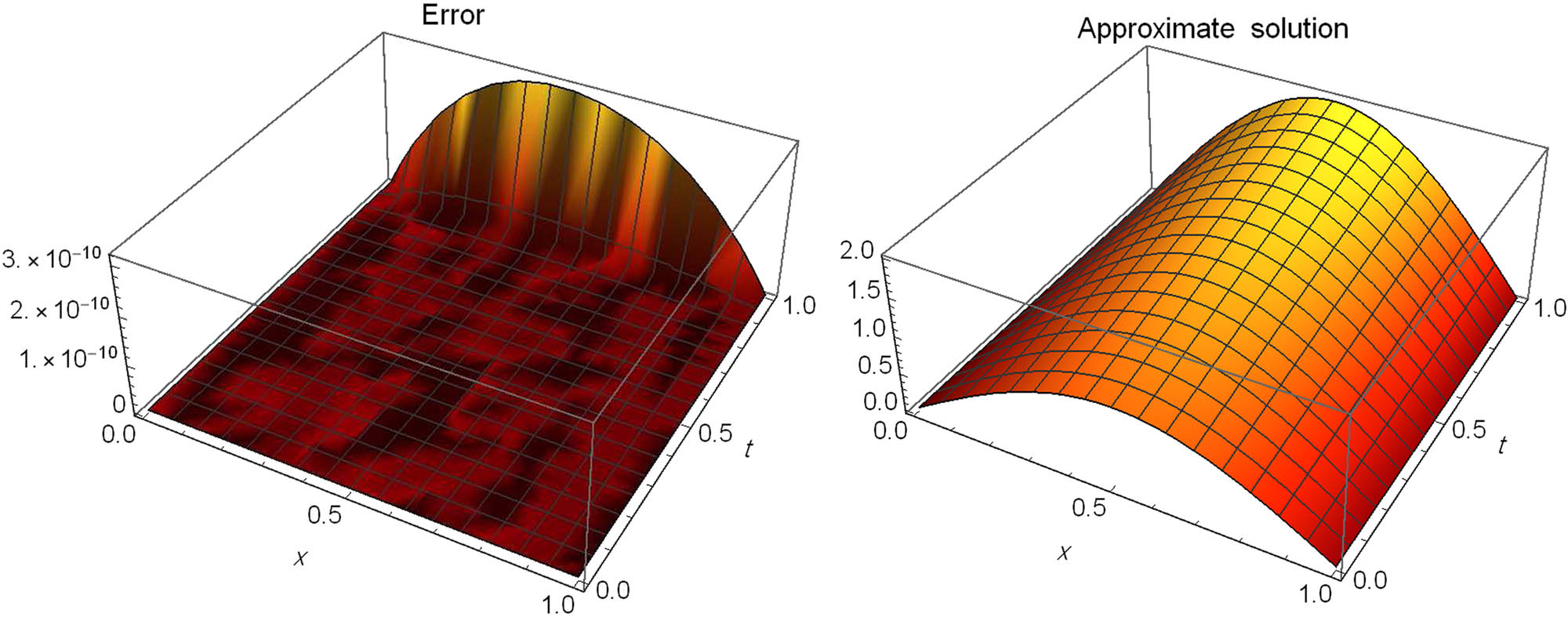
The AE (left) and approximate solution (right) for Test problem 1.
MAE for Test problem 1
|
|
|
|
|
|
|
|---|---|---|---|---|---|
| Error |
|
|
|
|
|
Test Problem 2
[33] Consider the TF4PDE of the form
subject to the following initial and boundary conditions:
where
Table 4 presents a comparison of MAE between our method and the method followed by Roul and Goura [33] at different values of
Comparison of the MAE for Test problem 2
|
|
Method in ref. [33] at
|
Our method at
|
|---|---|---|
| 0.4 |
|
|
| 0.5 |
|
|
| 0.7 |
|
|
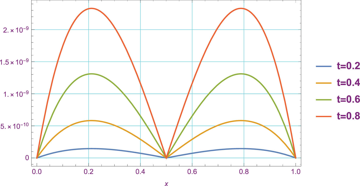
The AE for Test problem 2.
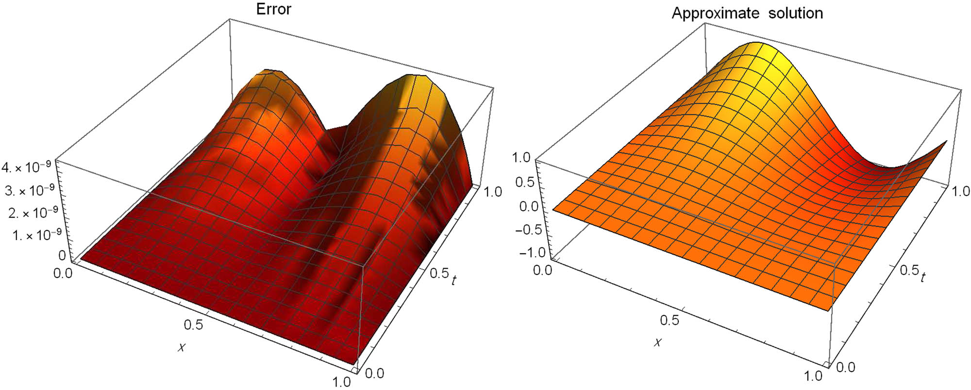
The AE (left) and approximate solution (right) for Test problem 2.
Test Problem 3
Consider the TF4PDE of the form
subject to the following initial and boundary conditions:
where
Table 5 reports the MAE at different values of
MAE for Test problem 3
| M | 2 | 4 | 6 | 8 | 10 | 12 |
|---|---|---|---|---|---|---|
| Error |
|
|
|
|
|
|
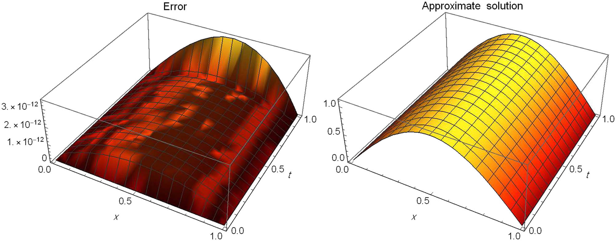
The AE (left) and approximate solution (right) for Test problem 3.
MAE for Test problem 3
|
|
|
|
|
|
|
|---|---|---|---|---|---|
| Error |
|
|
|
|
|
6 Concluding remarks
Herein, the time fractional fourth-order Euler–Bernoulli pinned–pinned beam was studied via a compact combination of Chebyshev polynomials as its spatial basis. The approach is based on discretizing the differential problem into a set of linear algebraic equations with unknown expansion coefficients using the Petrov–Galerkin algorithm. We solve the resulting system of equations with matrices that follow a specific pattern using the effective Gaussian elimination approach. The error bound is estimated. The theoretical analysis and effectiveness of the recently created algorithm are supported by numerical evidence. We plan to generalize the offered algorithm to more general differential problems in the near future. As an expected future work, we aim to employ the developed theoretical results in this article along with suitable spectral methods to treat more advanced problems, for instance, ref. [41]. All codes were written and debugged by Mathematica 11 on HP Z420 Workstation, Processor: Intel (R) Xeon(R) CPU E5-1620 – 3.6 GHz, 16 GB Ram DDR3, and 512 GB storage.
Acknowledgments
The authors would like to thank the anonymous reviewers for carefully reading the article and providing constructive and valuable comments that have improved the article’s present form.
-
Funding information: The authors received no financial support for the research.
-
Author contributions: All authors contributed equally to the work.
-
Conflict of interest: The authors declare that they have no conflict of interest.
-
Data availability statement: The authors did not use any scientific data during this research.
References
[1] Podlubny I. Fractional: an introduction to fractional derivatives, fractional, to methods of their solution and some of their applications. Amsterdam, The Netherlands: Elsevier; 1998. Search in Google Scholar
[2] Hilfer R. Applications of fractional calculus in physics. Singapore: World Scientific; 2000. 10.1142/3779Search in Google Scholar
[3] Kaur A, Kumar A. A new method for solving fuzzy transportation problems using ranking function. Appl Math Modell. 2011;35(12):5652–61. 10.1016/j.apm.2011.05.012Search in Google Scholar
[4] Abd-Elhameed WM, Napoli A. A unified approach for solving linear and nonlinear odd-order two-point boundary value problems. Bull Malays Math Sci Soc. 2020;43:2835–49. 10.1007/s40840-019-00840-7Search in Google Scholar
[5] Shokri J, Pishbin S. Study of fourth-order boundary value problem based on Volterra–Fredholm equation: numerical treatment. Inverse Probl Sci Eng. 2021;29(13):2862–76. 10.1080/17415977.2021.1954178Search in Google Scholar
[6] Atta AG, Abd-Elhameed WM, Moatimid GM, Youssri YH. Novel spectral schemes to fractional problems with nonsmooth solutions. Math Methods Appl Sci. 2023. 10.1002/mma.9343.Search in Google Scholar
[7] Fahad HM, Ur Rehman M, Fernandez A. On Laplace transforms with respect to functions and their applications to fractional differential equations. Math Methods Appl Sci. 2023;46(7):8304–23. 10.1002/mma.7772Search in Google Scholar
[8] Fernandez A, Restrepo JE, Suragan D. A new representation for the solutions of fractional differential equations with variable coefficients. Mediterr J Math. 2023;20(1):27. 10.1007/s00009-022-02228-7Search in Google Scholar
[9] Sajjadi SA, Najafi HS, Aminikhah H. A numerical study on the non-smooth solutions of the nonlinear weakly singular fractional Volterra integro-differential equations. Math Methods Appl Sci. 2023;46(4):4070–84. 10.1002/mma.8741Search in Google Scholar
[10] Sun ZZ, Gao Gh. Fractional Differential Equations: Finite Difference Methods. Berlin, Germany: De Gruyter; 2020.10.1515/9783110616064Search in Google Scholar
[11] Han SM, Benaroya H, Wei T. Dynamics of transversely vibrating beams using four engineering theories. J Sound Vib. 1999;225(5):935–88. 10.1006/jsvi.1999.2257Search in Google Scholar
[12] Aziz T, Khan A, Rashidinia J. Spline methods for the solution of fourth-order parabolic partial differential equations. Appl Math Comput. 2005;167(1):153–66. 10.1016/j.amc.2004.06.095Search in Google Scholar
[13] Evans DJ. A stable explicit method for the finite-difference solution of a fourth-order parabolic partial differential equation. Comput J. 1965;8(3):280–7. 10.1093/comjnl/8.3.280Search in Google Scholar
[14] Andrade C, McKee S. High accuracy A.D.I. methods for fourth order parabolic equations with variable coefficients. J Comput Appl Math. 1977;3(1):11–4. 10.1016/0771-050X(77)90019-5Search in Google Scholar
[15] Evans DJ, Yousif WS. A note on solving the fourth order parabolic equation by the age method. Int J Comput Math. 1991;40(1–2):93–7. 10.1080/00207169108804004Search in Google Scholar
[16] Wazwaz AM. Analytic treatment for variable coefficient fourth-order parabolic partial differential equations. Appl Math Comput. 2001;123(2):219–27. 10.1016/S0096-3003(00)00070-9Search in Google Scholar
[17] Doha EH, Bassuony MA, Abd-Elhameed WM, Youssri YH. A Legendre-Laguerre-Galerkin method for uniform Euler-Bernoulli beam equation. East Asian J Appl Math. 2018;8(2):280–95. 10.4208/eajam.060717.140118aSearch in Google Scholar
[18] Youssri YH, Muttardi MM. A mingled tau-finite difference method for stochastic first-order partial differential equations. Int J Appl Comput Math. 2023;9(2):14. 10.1007/s40819-023-01489-4Search in Google Scholar
[19] Youssri YH, Atta AG. Spectral collocation approach via normalized shifted Jacobi polynomials for the nonlinear Lane–Emden equation with fractal-fractional derivative. Fractal Fract. 2023;7(2):133. Search in Google Scholar
[20] Atta AG, Abd-Elhameed WM, Moatimid GM, Youssri YH. Shifted fifth-kind Chebyshev Galerkin treatment for linear hyperbolic first-order partial differential equations. Appl Numer Math. 2021;167:237–56. 10.1016/j.apnum.2021.05.010Search in Google Scholar
[21] Youssri YH, Abd-Elhameed WM, Sayed SM. Generalized Lucas tau method for the numerical treatment of the one and two-dimensional partial differential heat equation. J Funct Spaces. 2022;2022:13. 10.1155/2022/3128586Search in Google Scholar
[22] Youssri YH, Atta AG. Petrov-Galerkin Lucas polynomials procedure for the time-fractional diffusion equation. Contemp Math. 2023;4(2):230–48. 10.37256/cm.4220232420Search in Google Scholar
[23] Abd-Elhameed WM, Alkenedri AM. Spectral solutions of linear and nonlinear BVPS using certain Jacobi polynomials generalizing third-and fourth-kinds of Chebyshev polynomials. CMES-Comp Model Eng Sci. 2021;126(3):35. 10.32604/cmes.2021.013603Search in Google Scholar
[24] Jie S. Efficient spectral-Galerkin ii. direct solvers for second-and fourth-order equations by using Chebyshev polynomials. SIAM J. Sci. Comput. 1995;16:74–87. 10.1137/0916006Search in Google Scholar
[25] Abd-Elhameed WM, Alkenedri AM. New formulas for the repeated integrals of some Jacobi polynomials: spectral solutions of even-order boundary value problems. Int J Appl Comput Math. 2021;7(4):166. 10.1007/s40819-021-01109-zSearch in Google Scholar
[26] Abdelghany EM, Abd-Elhameed WM, Moatimid GM, Youssri YH, Atta AG. A tau approach for solving time-fractional heat equation based on the shifted sixth-kind Chebyshev polynomials. Symmetry. 2023;15(3):594. 10.3390/sym15030594Search in Google Scholar
[27] Abd-Elhameed WM, Alkhamisi SO, Amin AK, Youssri YH. Numerical contrivance for Kawahara-type differential equations based on fifth-kind Chebyshev polynomials. Symmetry. 2023;15(1):138. 10.3390/sym15010138Search in Google Scholar
[28] Youssri YH, Abd-Elhameed WM, Atta AG. Spectral Galerkin treatment of linear one-dimensional telegraph type problem via the generalized Lucas polynomials. Arabian J Mat. 2022;11(3):601–15. 10.1007/s40065-022-00374-0Search in Google Scholar
[29] Mason JC, Handscomb DC. Chebyshev polynomials. London: Chapman and Hall/CRC; 2002. 10.1201/9781420036114Search in Google Scholar
[30] Moustafa M, Youssri YH, Atta AG. Explicit Chebyshev-Galerkin scheme for the time-fractional diffusion equation. Int J Mod Phys C. 2023. 10.1142/S0129183124500025.Search in Google Scholar
[31] Atta AG, Youssri YH. Advanced shifted first-kind Chebyshev collocation approach for solving the nonlinear time-fractional partial integro-differential equation with a weakly singular kernel. Comput Appl Math. 2022;41(8):381. 10.1007/s40314-022-02096-7Search in Google Scholar
[32] Youssri YH, Atta AG. Double Tchebyshev spectral tau algorithm for solving KdV equation, with soliton application. In: Helal MA, editor. Solitons. New York (NY), USA: Springer US; 2022. p. 451. 10.1007/978-1-0716-2457-9_771Search in Google Scholar
[33] Roul P, Goura VMKP. A high order numerical method and its convergence for time-fractional fourth-order partial differential equations. Appl Math Comput. 2020;366:124727. 10.1016/j.amc.2019.124727Search in Google Scholar
[34] Abd-Elhameed WM, Machado JAT, Youssri YH. Hypergeometric fractional derivatives formula of shifted Chebyshev polynomials: tau algorithm for a type of fractional delay differential equations. Int J Nonlinear Sci Numer Simul. 2022;23(7–8):1253–68. 10.1515/ijnsns-2020-0124Search in Google Scholar
[35] Bhrawy AH, Zaky MA. A method based on the Jacobi tau approximation for solving multi-term time-space fractional partial differential equations. J Comput Phys. 2015;281:876–95. 10.1016/j.jcp.2014.10.060Search in Google Scholar
[36] Youssri YH, Atta AG. Spectral collocation approach via normalized shifted Jacobi polynomials for the nonlinear Lane–Emden equation with fractal-fractional derivative. Fractal Fract. 2023;7(2):133. 10.3390/fractalfract7020133Search in Google Scholar
[37] Sadri K, Aminikhah H. Chebyshev polynomials of sixth kind for solving nonlinear fractional PDEs with proportional delay and its convergence analysis. J Funct Spaces. 2022;2022:1–20. 10.1155/2022/9512048Search in Google Scholar
[38] Zhao X, Wang L, Xie Z. Sharp error bounds for Jacobi expansions and Gegenbauer-Gauss quadrature of analytic functions. SIAM J Numer Anal. 2013;51(3):1443–69. 10.1137/12089421XSearch in Google Scholar
[39] Siddiqi SS, Arshed S. Numerical solution of time-fractional fourth-order partial differential equations. Int J Comput Math. 2015;92(7):1496–518. 10.1080/00207160.2014.948430Search in Google Scholar
[40] Tariq H, Akram G. Quintic spline technique for time fractional fourth-order partial differential equation. Numer Methods Partial Differ Equ. 2017;33(2):445–66. 10.1002/num.22088Search in Google Scholar
[41] Mostafa D, Zaky MA, Hafez RM, Hendy AS, Abdelkawy MA, Aldraiweesh AA. Tanh Jacobi spectral collocation method for the numerical simulation of nonlinear Schrödinger equations on unbounded domain. Math Methods Appl Sci. 2023;46(1):656–74. 10.1002/mma.8538Search in Google Scholar
© 2023 the author(s), published by De Gruyter
This work is licensed under the Creative Commons Attribution 4.0 International License.
Articles in the same Issue
- Research Articles
- The regularization of spectral methods for hyperbolic Volterra integrodifferential equations with fractional power elliptic operator
- Analytical and numerical study for the generalized q-deformed sinh-Gordon equation
- Dynamics and attitude control of space-based synthetic aperture radar
- A new optimal multistep optimal homotopy asymptotic method to solve nonlinear system of two biological species
- Dynamical aspects of transient electro-osmotic flow of Burgers' fluid with zeta potential in cylindrical tube
- Self-optimization examination system based on improved particle swarm optimization
- Overlapping grid SQLM for third-grade modified nanofluid flow deformed by porous stretchable/shrinkable Riga plate
- Research on indoor localization algorithm based on time unsynchronization
- Performance evaluation and optimization of fixture adapter for oil drilling top drives
- Nonlinear adaptive sliding mode control with application to quadcopters
- Numerical simulation of Burgers’ equations via quartic HB-spline DQM
- Bond performance between recycled concrete and steel bar after high temperature
- Deformable Laplace transform and its applications
- A comparative study for the numerical approximation of 1D and 2D hyperbolic telegraph equations with UAT and UAH tension B-spline DQM
- Numerical approximations of CNLS equations via UAH tension B-spline DQM
- Nonlinear numerical simulation of bond performance between recycled concrete and corroded steel bars
- An iterative approach using Sawi transform for fractional telegraph equation in diversified dimensions
- Investigation of magnetized convection for second-grade nanofluids via Prabhakar differentiation
- Influence of the blade size on the dynamic characteristic damage identification of wind turbine blades
- Cilia and electroosmosis induced double diffusive transport of hybrid nanofluids through microchannel and entropy analysis
- Semi-analytical approximation of time-fractional telegraph equation via natural transform in Caputo derivative
- Analytical solutions of fractional couple stress fluid flow for an engineering problem
- Simulations of fractional time-derivative against proportional time-delay for solving and investigating the generalized perturbed-KdV equation
- Pricing weather derivatives in an uncertain environment
- Variational principles for a double Rayleigh beam system undergoing vibrations and connected by a nonlinear Winkler–Pasternak elastic layer
- Novel soliton structures of truncated M-fractional (4+1)-dim Fokas wave model
- Safety decision analysis of collapse accident based on “accident tree–analytic hierarchy process”
- Derivation of septic B-spline function in n-dimensional to solve n-dimensional partial differential equations
- Development of a gray box system identification model to estimate the parameters affecting traffic accidents
- Homotopy analysis method for discrete quasi-reversibility mollification method of nonhomogeneous backward heat conduction problem
- New kink-periodic and convex–concave-periodic solutions to the modified regularized long wave equation by means of modified rational trigonometric–hyperbolic functions
- Explicit Chebyshev Petrov–Galerkin scheme for time-fractional fourth-order uniform Euler–Bernoulli pinned–pinned beam equation
- NASA DART mission: A preliminary mathematical dynamical model and its nonlinear circuit emulation
- Nonlinear dynamic responses of ballasted railway tracks using concrete sleepers incorporated with reinforced fibres and pre-treated crumb rubber
- Two-component excitation governance of giant wave clusters with the partially nonlocal nonlinearity
- Bifurcation analysis and control of the valve-controlled hydraulic cylinder system
- Engineering fault intelligent monitoring system based on Internet of Things and GIS
- Traveling wave solutions of the generalized scale-invariant analog of the KdV equation by tanh–coth method
- Electric vehicle wireless charging system for the foreign object detection with the inducted coil with magnetic field variation
- Dynamical structures of wave front to the fractional generalized equal width-Burgers model via two analytic schemes: Effects of parameters and fractionality
- Theoretical and numerical analysis of nonlinear Boussinesq equation under fractal fractional derivative
- Research on the artificial control method of the gas nuclei spectrum in the small-scale experimental pool under atmospheric pressure
- Mathematical analysis of the transmission dynamics of viral infection with effective control policies via fractional derivative
- On duality principles and related convex dual formulations suitable for local and global non-convex variational optimization
- Study on the breaking characteristics of glass-like brittle materials
- The construction and development of economic education model in universities based on the spatial Durbin model
- Homoclinic breather, periodic wave, lump solution, and M-shaped rational solutions for cold bosonic atoms in a zig-zag optical lattice
- Fractional insights into Zika virus transmission: Exploring preventive measures from a dynamical perspective
- Rapid Communication
- Influence of joint flexibility on buckling analysis of free–free beams
- Special Issue: Recent trends and emergence of technology in nonlinear engineering and its applications - Part II
- Research on optimization of crane fault predictive control system based on data mining
- Nonlinear computer image scene and target information extraction based on big data technology
- Nonlinear analysis and processing of software development data under Internet of things monitoring system
- Nonlinear remote monitoring system of manipulator based on network communication technology
- Nonlinear bridge deflection monitoring and prediction system based on network communication
- Cross-modal multi-label image classification modeling and recognition based on nonlinear
- Application of nonlinear clustering optimization algorithm in web data mining of cloud computing
- Optimization of information acquisition security of broadband carrier communication based on linear equation
- A review of tiger conservation studies using nonlinear trajectory: A telemetry data approach
- Multiwireless sensors for electrical measurement based on nonlinear improved data fusion algorithm
- Realization of optimization design of electromechanical integration PLC program system based on 3D model
- Research on nonlinear tracking and evaluation of sports 3D vision action
- Analysis of bridge vibration response for identification of bridge damage using BP neural network
- Numerical analysis of vibration response of elastic tube bundle of heat exchanger based on fluid structure coupling analysis
- Establishment of nonlinear network security situational awareness model based on random forest under the background of big data
- Research and implementation of non-linear management and monitoring system for classified information network
- Study of time-fractional delayed differential equations via new integral transform-based variation iteration technique
- Exhaustive study on post effect processing of 3D image based on nonlinear digital watermarking algorithm
- A versatile dynamic noise control framework based on computer simulation and modeling
- A novel hybrid ensemble convolutional neural network for face recognition by optimizing hyperparameters
- Numerical analysis of uneven settlement of highway subgrade based on nonlinear algorithm
- Experimental design and data analysis and optimization of mechanical condition diagnosis for transformer sets
- Special Issue: Reliable and Robust Fuzzy Logic Control System for Industry 4.0
- Framework for identifying network attacks through packet inspection using machine learning
- Convolutional neural network for UAV image processing and navigation in tree plantations based on deep learning
- Analysis of multimedia technology and mobile learning in English teaching in colleges and universities
- A deep learning-based mathematical modeling strategy for classifying musical genres in musical industry
- An effective framework to improve the managerial activities in global software development
- Simulation of three-dimensional temperature field in high-frequency welding based on nonlinear finite element method
- Multi-objective optimization model of transmission error of nonlinear dynamic load of double helical gears
- Fault diagnosis of electrical equipment based on virtual simulation technology
- Application of fractional-order nonlinear equations in coordinated control of multi-agent systems
- Research on railroad locomotive driving safety assistance technology based on electromechanical coupling analysis
- Risk assessment of computer network information using a proposed approach: Fuzzy hierarchical reasoning model based on scientific inversion parallel programming
- Special Issue: Dynamic Engineering and Control Methods for the Nonlinear Systems - Part I
- The application of iterative hard threshold algorithm based on nonlinear optimal compression sensing and electronic information technology in the field of automatic control
- Equilibrium stability of dynamic duopoly Cournot game under heterogeneous strategies, asymmetric information, and one-way R&D spillovers
- Mathematical prediction model construction of network packet loss rate and nonlinear mapping user experience under the Internet of Things
- Target recognition and detection system based on sensor and nonlinear machine vision fusion
- Risk analysis of bridge ship collision based on AIS data model and nonlinear finite element
- Video face target detection and tracking algorithm based on nonlinear sequence Monte Carlo filtering technique
- Adaptive fuzzy extended state observer for a class of nonlinear systems with output constraint