Nonlinear adaptive sliding mode control with application to quadcopters

Ryan Mathewson; Farbod Fahimi

doi:10.1515/nleng-2022-0268

Article Open Access

Nonlinear adaptive sliding mode control with application to quadcopters

Ryan Mathewson and Farbod Fahimi

Published/Copyright: February 28, 2023

Published by

Become an author with De Gruyter Brill

Submit Manuscript Author Information

From the journal Nonlinear Engineering Volume 12 Issue 1

Abstract

Nonlinear adaptive sliding mode control (NASMC) has the capability to adequately control a system whose parameters are unknown to the controller designer. Conventional model-based controllers require a mathematical dynamic model of the system with known parameters. These system parameters are normally determined by extensive system identification experiments, which are expensive and time-consuming to perform. A NASMC approach that does not require known system parameters is proposed. Using NASMC, a controller designer can skip the expensive and time-consuming system parameter identification and fast-forward to the control implementation. In addition, once a controller is derived for a quadcopter using NASMC, the same controller will work on any quadcopter with the same equations of motion but different dynamic parameters. The formulation of the NASMC is presented for general second-order and fourth-order systems. Then, as an implementation example, the application of the general NASMC approach is demonstrated by applying it to a quadcopter unmanned aerial vehicle in simulation.

Keywords: nonlinear control; nth-order adaptive variable structure control; fourth-order quadcopter model; single-loop quadcopter control; unknown system parameters

1 Introduction

Adaptive control has been successfully developed for certain types of nonlinear control problems. The proposed nonlinear adaptive sliding mode controller (NASMC) is shown to be very powerful when the nonlinear plant dynamics can be linearly parameterized and the state is measurable. This thesis attempts to show the advantages and power of the proposed reformulated NASMC approach through a demonstration of the NASMC application to a quadcopter system.

1.1 Brief literature survey

Quadcopters have an extremely broad range of uses, whether they be for commercial, government, or educational purposes. Many researchers have been working to provide more stable operations for a larger range of circumstances using improved modeling, estimation of states, and control techniques [1–3]. Nonlinear controllers are much more desirable for their ability to expand the range of operation and the robustness of the controller. Most of the algorithms that use these approaches suffer from disadvantages that the NASMC can account for. These include things like a lack of robustness to external disturbances and reliance on simplified quadcopter dynamics.

Figure 1

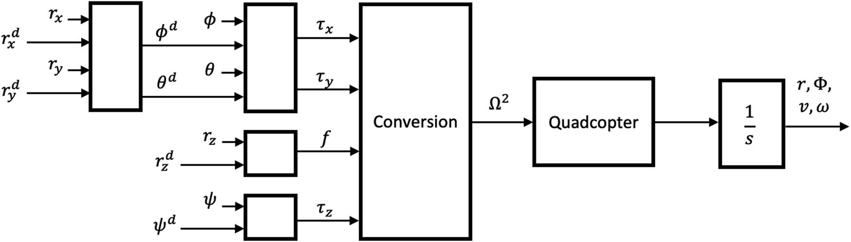
Basic cascade structure block diagram for quadcopter.

Many researchers that have worked on this problem in the past have taken advantage of the cascade structure of quadcopter dynamics and developed nonlinear controllers based on it (Figure 1). The big disadvantage of the cascade structure is that it only shows that the position tracking errors are bounded but not asymptotically stabilized. This is due to the indirect control of the control moments τ x and τ y by using the r x and r y positions to control the roll and pitch angles, which in turn are what control τ . Using this method can lead to potential instabilities, which would be undesirable.

There are various different design techniques for quadcopter control that use the cascade structure, including methods like feedback linearization and backstepping [4–8], Lyapunov functions [9,10], sliding mode control [11–14], robust adaptive and geometric tracking control [15–19], and other methods completely [20]. Many of these works are based on simplifying assumptions or creating other restrictions on the system. As an example, previous studies [4,9,11,12,21] all choose in their approach to neglect the difference between orientation angle rates and angular velocities/accelerations.

In some research, the approach has concentrated on attitude stabilization without robust trajectory tracking stabilization like in previous studies [18,22–24]. The biggest problem with attitude stabilization is that to achieve zero tracking error, one must perfectly know the relationship between attitude angles and translational motion. These relationships have thus been presented without any disturbances or uncertainties as in the studies of Yu et al. [8] and Zhao et al. [19], which include uncertainties and disturbances in angular motion but ignore them in translational motion. In addition, the studies of Choi and Ahn [7] and Yu and Ding [24] both suggest an adaptive control to estimate the uncertainties and disturbances in translational motion, but do not go into further discussion on the topic. A second-order sliding mode controller was suggested in the study of Zheng et al. [21]; however, the authors chose not to include uncertainties in the model, and the sliding surfaces that are suggested are not necessarily asymptotically stable. Another method, as in the study of Lee et al. [17], includes unknown disturbances in the model, but it uses the cascade control structure, demonstrating that the position-tracking errors are bounded but not asymptotically stabilized. Every article in the aforementioned reference sets uses τ x and τ y to control the pitch and roll of the vehicle, which in turn only indirectly controls x and y . This lack of direct control leads to only achieving bounded errors of x and y .

An improved technique, as discussed extensively in the study of Poultney et al. [25], is the introduction of a pair of two second-order and two fourth-order subsystems that work in tandem to control a quadcopter. This technique is not utilized in any other reference within this document. The fourth-order subsystems are used to directly control x and y using τ x and τ y . This allows the system to achieve asymptotically stable x and y errors in a way that the other referenced research has not been able to achieve. The work of Poultney et al. [25] is built upon and discussed extensively in this article due to the novelty of the multiple-ordered subsystems technique working to reduce errors.

1.2 Motivation and contributions

The NASMC techniques presented here are derived from Slotine and Li’s [26] work, which discusses adaptive control of nonlinear systems. The formulations and methods presented were combined with that in the study of Slotine and Coetsee [27], which is also co-written by Slotine, and re-derived to include a detailed stability proof that was missing from the study of Slotine and Li [26] and was used to expand the NASMC approach used here.

There are many benefits to the NASMC approach that are not found in other methods. First, the advantage stated above, NASMC is able to achieve asymptotically stable x and y position errors, compared to the bounded errors achieved by other cited sources in Section 1.1. NASMC is also able to be generalized; it can be used with any number of ordered systems. All system orders can be formulated following the same approach.

One of the strongest aspects of the NASMC approach is that it does not require knowledge of system parameters to work. This means that, in general, a NASMC approach is strongly desirable to increase the range of operations. By not requiring the knowledge of system parameters, it eliminates the need to perform system identification experiments, which would normally be used to find such parameters. The controller is designed as if the unknown parameters were actually known exactly, but since this is not initially the case, the system wanders outside the boundary layer to eventually improve the parameter estimates. Once inside the boundary layer, the system understands that no further advantage is gained by continuing adaptation. Even if the parameters are still not known exactly, they can successfully eliminate the combined error.

The NASMC approach also adapts to gradual changes in system parameters. These changes can happen due to a number of factors, which include the aging of the system, changes in the environment, and more depending on the application. This can also reduce the number of sensors required in a system, which may no longer be required to measure these parameters. In addition, the NASMC approach is scalable, requiring no changes when implemented to other systems of similar type that use the same equations of motion but have different unknown parameters (e.g., the NASMC used on a small quadcopter could also be used on a large quadcopter with the same layout).

Some disadvantages of the NASMC approach exist. Slower tracking of the x and y subsystems occurs since they are higher order and take more time to adapt to the unknown parameters. The x and y subsystems also require knowledge of the third and fourth derivatives of the functions, which can be difficult to calculate and estimate.

To demonstrate the power of the proposed NASMC approach and its implementation, we apply it to a quadcopter in simulation as an example. The quadcopter is seen as a strong candidate for utilizing all the advantages of the approach due to its use in many different environments, its high potential for unknown disturbances, and because developing its dynamic system parameters is a difficult and costly endeavor. A quadcopter also has many real-world applications ranging from simple toys to large-scale government operations that can take advantage of the ability to scale.

This NASMC approach provides significant advantages over other methods in terms of tracking performance and unknown parameter estimation. The ability to scale and avoid system identification experiments also provide time and cost saving advantages in real-world applications. Finally, the performance of this controller shows strong potential for further research and experimentation on any number of systems.

1.3 Summary of the key contributions

The key contributions of the article are as follows:

An alternative, detailed stability analysis is presented for NASMC that is missing in the literature.
The alternative, detailed stability analysis defines a residual error whose decay to zero is proven (and demonstrated in examples), whereas the stability analysis in the literature only proves bounded errors for parameter estimation errors.
An adaptive single-loop control method is derived for a quadcopter, whereas only nonadaptive multi-loop controllers or some nonadaptive single-loop controllers are found in the literature.
The adaptive nature of the proposed controller eliminates any need for extensive and time-consuming system identifications tests.
The single-loop nature of the proposed controller simplifies the architecture of the controller implementation compared to that of multi-loop controllers.
Fourth-order subsystems are used to control the x and y states, which achieve asymptotic convergence to zero error in these states, whereas the second-order controllers used in the literature for the x and y states only achieve bounded (nonzero) errors for these states.

2 Assumptions made

There are a few assumptions that are made in this article about how the quadcopter is controlled. It is assumed that the quadcopter’s geometry has two planes of symmetry. As a consequence, we are choosing to neglect the off-diagonal elements of the mass moment of inertia matrix I . Furthermore, we assume that rotor thrusts and rotor drag torques are linear with the square of rotor speeds ( Ω 2 ). Finally, we are making the assumption that the location of the center of mass (CM) of the quadcopter is known.

3 Methods

The chosen method of control for the quadcopter is a NASMC, which offers robustness in relation to parametric uncertainty. The controllers will control the system with unknown constants or very slowly varying parameters. This is because parameters are hard to determine through experimentation and could vary due to use conditions and age of the vehicle. For the simulation presented, both second- and fourth-order controllers are used.

3.1 Adaptive sliding mode controller used

For the general nth-order controller, consider the following dynamic system:

(1) y ( n ) + ∑ i = 1 n α i f i = b u + δ ,

where y ( n ) is the nth time derivative of position, u ( t ) is the control input, δ is the disturbance term, f i are known nonlinear functions of the state and time, and α i and b are unknown system parameters. Solving for the control input, this equation can then be rewritten as follows:

(2) h y ( n ) + ∑ i = 1 n a i f i + d = u ,

where h = 1 / b , a i = α i / b , and d = − δ / b .

Let us define a combined error:

(3) s = e ( n − 1 ) + ∑ i = 0 n − 2 n − 1 i λ n − i − 1 e i ,

where e is the output tracking error. Note that when s vanishes in Eq. (3), for any λ > 0 , the error exponentially approaches zero. Later, it will be proven that, by a correct choice of the control law, s exponentially vanishes. For further use, s can be rewritten as follows:

(4) s = y ( n − 1 ) − y r ( n − 1 ) ,

where the reference value y r ( n − 1 ) is defined as

(5) y r ( n − 1 ) = y d ( n − 1 ) − ∑ i = 0 n − 2 n − 1 i λ n − i − 1 e i ,

where y d ( n − 1 ) is the desired value. To yield a robust adaptive controller, we replace s with

(6) s Δ = s − ϕ s sat ( s / ϕ s ) ,

which measures the algebraic distance of the current state to the boundary layer, where ϕ s is the boundary layer thickness and

(7) sat ( s / ϕ s ) = − 1 if s ≤ − ϕ s , s / ϕ s if − ϕ s < s < ϕ s , 1 if s ≥ ϕ s .

The boundary layer is a region around s = 0 in which the finite time convergence of s transforms into exponential convergence.

3.1.1 Derivation of control law for known system parameters

First, a nonadaptive sliding mode control (SMC) is considered. For the nonadaptive SMC, we assume that the system parameters, h and a i , are known. To make sure s vanishes with time, we propose the following control law:

(8) u = h y r ( n ) − k s + ∑ i = 1 n a i f i ,

where k is chosen as a constant of the same sign as h and

(9) y r ( n ) = y d ( n ) − ∑ i = 0 n − 2 n − 1 i λ n − i − 1 e i + 1 ,

where y r ( n ) is the reference value of y ( n ) .

First, we prove that, if the system parameters h and a i are known and there is no disturbance (i.e., d = 0 ), s exponentially approaches zero. This is done by substituting Eq. (8) in Eq. (1) and simplifying the result. The simplification yields the following tracking error dynamics:

(10) s ˙ + ( k / h ) s = 0 .

Note that, since h and k have the same sign, k / h > 0 , which leads to the exponential convergence of s .

3.1.2 Derivation of control law for unknown system parameters

Second, a NASMC is considered. For the NASMC approach, the system parameters are unknown, and we set our control law to include the estimated values of h ˆ and a ˆ i :

(11) u = h ˆ y r ( n ) − k s + ∑ i = 1 n a ˆ i f i .

By substituting Eq. (11) into Eq. (1), assuming there is no disturbance, and simplifying the result, s again exponentially approaches zero. The tracking error dynamics then become

(12) h s ˙ + k s = ρ n ,

(13) ρ n = h ˜ y r ( n ) + ∑ i = 1 n a ˜ i f i ,

where ρ n is the residual error due to parameter estimation, and h ˜ = h ˆ − h and a ˜ i = a ˆ i − a i are the parameter estimation errors.

Note that, in Eqs. (12) and (13), s only vanishes if the residual error ρ n vanishes. In the following section, we discuss the adaptation laws for the unknown parameters that yield the elimination of parameter estimation errors.

3.1.3 Derivation of adaptation laws and stability analysis

To derive a control law that ensures convergence to the boundary layer, a Lyapunov function candidate V ( t ) is defined as follows:

(14) V ( t ) = 1 2 s Δ 2 + b h ˆ − h γ 0 2 + ∑ i = 1 n a ˆ i − a i γ i 2 ,

where h ˆ and a ˆ i are the estimated values of h and a i , respectively, and γ i are tuning gains. We then select the control law u as follows:

(15) u = h ˆ y r ( n ) − h ˆ ( D + η ) sat ( s / ϕ s ) + ∑ i = 1 n a ˆ i f i ,

where

(16) y r ( n ) = y d ( n ) − ∑ i = 0 n − 2 n − 1 i λ n − i − 1 e i + 1 ,

D is the maximum disturbance, and η is the gain for sliding mode surface reaching phase. We will explore this further in the next section.

To properly find the time derivative of Eq. (14), the time derivative of s is required. Taking the derivative of Eq. (4), we obtain

(17) s ˙ = y ( n ) − y r ( n ) .

We then substitute Eqs. (1), (15), and (16) into Eq. (17) and simplify the result to obtain

(18) s ˙ = ∑ i = 1 n b f i ( a ˆ i − a i ) − ( b h ˆ − 1 ) y r ( n ) − b h ˆ ( D + η ) sat ( s / ϕ s ) + d .

When noting that s ˙ Δ = s ˙ outside the boundary layer and s Δ = 0 inside the boundary layer, taking the time derivative of Eq. (14) yields

(19) V ˙ ( t ) = s ˙ s Δ + b h ˆ ˙ γ 0 2 ( h ˆ − h ) + ∑ i = 1 n a ˆ ˙ i γ i 2 ( a ˆ i − a i ) ,

which we then substitute Eq. (18) and simplify to obtain

(20) V ˙ ( t ) = ( b h ˆ − 1 ) h ˆ ˙ γ 0 2 − y r ( n ) s Δ + ∑ i = 1 n a ˜ i b a ˆ ˙ i γ i 2 + f i s Δ − b h ˆ ( D + η ) s Δ sat ( s / ϕ s ) + d s Δ .

The adaptation laws are selected as follows:

(21) h ˆ ˙ = γ 0 2 s Δ ( y r ( n ) + ( D + η ) sat ( s / ϕ s ) )

and for i = 1 to n :

(22) a ˆ ˙ i = − γ i 2 f i s Δ .

This leads to the result

(23) V ˙ ( t ) = ( − ( D + η ) sat ( s / ϕ s ) + d ) s Δ ,

so that outside the boundary layer,

(24) V ˙ ( t ) ≤ − η ∣ s Δ ∣ .

V ˙ ( t ) is monotonically negative since we choose η > 0 and V ( t ) in Eq. (14) vanishes over time, which means that V ( t ) reaches a constant minimum. In other words, the residual error ρ n vanishes.

This controller will later be applied to a part of the quadcopter vehicle control system in both second- and fourth-order forms.

3.2 Quadcopter dynamics and model

This section will discuss the dynamics and equations required to create the quadcopter model in simulation. First, we must create the quadcopter model from the kinematic and dynamic relationships of the vehicle. Then, we will use the second- and fourth-order controllers as subsystems in the larger quadcopter model and present the control structure.

For the quadcopter, we consider a rigid body model in three-dimensional (3D) space with six degrees-of-freedom (DOF). We define an earth-fixed frame X e Y e Z e that is attached to some reference location and a body-fixed frame X Y Z that is attached to the quadcopter’s CM. When defining position and orientation of the quadcopter relative to the earth-fixed frame, we use the position vector r = [ x , y , z ] T and the orientation vector Φ = [ ϕ , θ , ψ ] T , where ϕ , θ , and ψ are roll, pitch, and yaw Euler angles, respectively. The orientation of these is shown in Figure 2. The orthogonal rotation matrix R allows us to relate the rigid body CM linear velocity vector in the earth-fixed frame V = [ V x , V y , V z ] T to the body-fixed frame velocity vector v = [ v x , v y , v z ] T , which are shown on the following equation:

(25) R = c θ c ψ c ϕ s ψ + s ϕ s θ c ψ s ϕ s ψ − c ϕ s θ c ψ − c θ s ψ c ϕ c ψ − s ϕ s θ s ψ s ϕ c ψ + c ϕ s θ s ψ s θ − s ϕ c θ c ϕ c θ

(26) r ˙ = V = R T v , v = R V ,

where s ϕ = sin ϕ and c ϕ = cos ϕ , and similarly for θ and ψ . The angular velocity vector in the body-fixed frame, ω , and the vector of Euler angle rates, Φ ˙ = [ ϕ ˙ , θ ˙ , ψ ˙ ] T are related through the following equations:

(27) ω = B Φ ˙ , Φ ˙ = B − 1 ω ,

where

(28) B = c θ c ψ s ψ 0 − c θ s ψ c ψ 0 s θ 0 1 ,

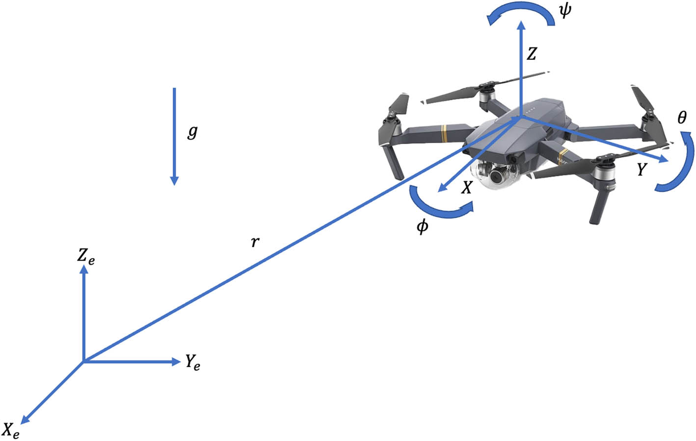
and since the B matrix becomes singular when θ = ± π / 2 , we restrict the inverse transformation to − π / 2 < θ < π / 2 .

Figure 2

Quadcopter reference frames.

The equations of motion for the quadcopter modeled as a rigid body are as follows:

(29) m v ˙ = F − m ω × v = F − m ω ˜ v I ω ˙ = T − ω × ( I ω ) = T − ω ˜ I ω ,

where m is the quadcopter mass, I = diag [ I x x , I y y , I z z ] is the mass moment of inertia matrix, F represents the external forces, T represents the external moments, and v ˙ and ω ˙ are the rigid body CM linear and acceleration vectors in the body-fixed frame. The tilde notation defines a skew-symmetric matrix from a vector as follows:

(30) ω ˜ = 0 − ω z ω y ω z 0 − ω x − ω y ω x 0 .

The 12 states of the system are the rigid body CM position relative to the earth-fixed frame ( r ) the Euler angles ( Φ ) the rigid body CM velocities in the body-fixed frame ( v ) and the rigid body angular velocities in the body-fixed frame ( ω ). Thus, Eqs. (26), (27), and (29), collectively, form 12 equations of state.

To find the total thrust control force, f , and the control moment vector, τ = [ τ x , τ y , τ z ] T , we consider a planar top view of the quadcopter as seen in Figure 3. The body-fixed frame X Y Z , located at the quadcopter CM, may not coincide with the geometrically centered frame which we define as X g Y g Z g . A vector to represent the position of the CM with respect to the geometric center is defined as r C M = [ x C M , y C M , z C M ] T . We now define the relationship between f , τ , and the individual rotor angular speeds, Ω i . This is dependent on the equivalent thrust coefficient, c T , and the torque coefficient, c Q , and is shown as follows:

(31) f τ x τ y τ z = c T c T c T c T d 4 c T − d 3 c T − d 3 c T d 4 c T d 1 c T − d 2 c T d 1 c T − d 2 c T − c Q − c Q c Q c Q Ω 1 2 Ω 2 2 Ω 3 2 Ω 4 2 ,

where d 1 = d / 2 + x C M , d 2 = d / 2 − x C M , d 3 = d / 2 + y C M , d 4 = d / 2 − y C M , and d is the distance from the geometric center to any individual rotor.

Figure 3

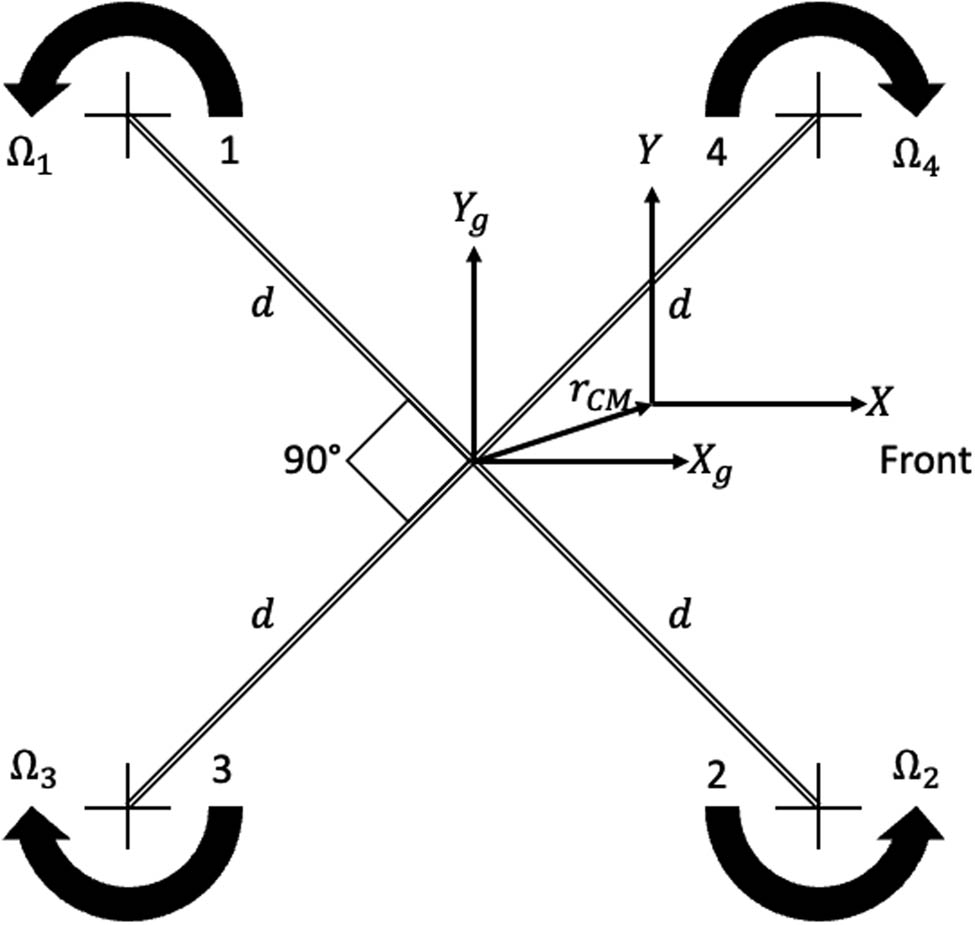
Quadcopter top view.

3.3 NASMC design

To create the NASMC system for our quadcopter example, we require derivations of the second- and fourth-order control subsystem equations.

3.3.1 Derivation of second-order and fourth-order control subsystems

To reach the roll and pitch moments τ x and τ y for use as inputs, we must use the fourth time derivative of the desired outputs x and y . This can be achieved through the system model for the translational part of the equations of motion in the earth-fixed frame. This is written as follows:

(32) m V ˙ = R T 0 0 f ˆ − 0 0 m g ,

where the thrust force used is the nominal value f ˆ . Taking the first and second time derivatives yields

(33) m V ¨ = R T 0 0 f ˆ ˙ + ω ˜ 0 0 f ˆ

(34) m V ⃜ = R T 0 0 f ˆ ¨ + 2 ω ˜ 0 0 f ˆ ˙ + ( ω ˜ ˙ + ω ˜ ω ˜ ) 0 0 f ˆ ,

where V ¨ and V ⃜ are called jerk and snap, respectively. Eq. (34) directly relates τ x and τ y to snap by substituting for ω ˙ x and ω ˙ y from Eq. (29). Note that ω ˙ z and thus τ z to not appear in Eq. (34).

For this control method, we must define some “ u ” parameters, which are u 1 , u 2 , u 3 , and u 4 . These parameters come from Eq. (31) and are useful as controlled parameters. The equation is separated and rewritten as follows, in addition to providing how they relate to the u i :

(35) f = c T ∑ i = 1 4 Ω i 2 = c T u 1 τ x = c T ( d 4 Ω 1 2 + d 4 Ω 4 2 − d 3 Ω 2 2 − d 3 Ω 3 2 ) = c T u 2 τ y = c T ( d 1 Ω 1 2 + d 1 Ω 3 2 − d 2 Ω 2 2 − d 2 Ω 4 2 ) = c T u 3 τ z = c Q ( Ω 3 2 + Ω 4 2 − Ω 1 2 − Ω 2 2 ) = c Q u 4 .

These equations will help us relate the thrust control force and the control moments to the position and yaw angle.

Next, we rewrite the equations of motion in Eq. (29) without the unknown terms and in detailed form:

(36) v ˙ x = ω z v y − ω y v z − g R 13 v ˙ y = ω x v z − ω z v x − g R 23 v ˙ z = ω y v x − ω x v y − g R 33 + f ˆ / m

(37) ω ˙ x = [ τ x − ( I z z − I y y ) ω y ω z ] / I x x ω ˙ y = [ τ y − ( I x x − I z z ) ω z ω x ] / I y y ω ˙ z = [ τ z − ( I y y − I x x ) ω x ω y ] / I z z ,

with R i j indicating the i , j element of R in Eq. (25).

To put Eq. (34) into a form that will work for our simulation example, we must utilize the property of Eq. (26) to solve for r .... . Since we only need to use the fourth time derivative of position for x and y , we only need the portions of the equation for solving r .... x and r .... y and the last line for z may be ignored. This leads to:

(38) r x .... = R 11 2 ω y f ˆ ˙ m + c T u 3 − ( I x x − I z z ) ω z ω x I x x y y + ω z ω x f ˆ m + R 21 − 2 ω x f ˆ ˙ m + − c T u 2 − ( I z z − I y y ) ω y ω z I x x y y + ω z ω y f ˆ m + R 31 f ˆ ¨ m + ( − ω y 2 − ω x 2 ) f ˆ m

(39) r y .... = R 12 2 ω y f ˆ ˙ m + c T u 3 − ( I x x − I z z ) ω z ω x I x x y y + ω z ω x f ˆ m + R 22 − 2 ω x f ˆ ˙ m + − c T u 2 − ( I z z − I y y ) ω y ω z I x x y y + ω z ω y f ˆ m + R 32 f ˆ ¨ m + ( − ω y 2 − ω x 2 ) f ˆ m ,

where we must make the assumption that I x x = I y y = I x x y y , though this does not have to be the case in the real application. Similarly, r ¨ z can be solved by again substituting in Eq. (26), this time into Eq. (32), and taking only the last line to become

(40) r ¨ z = R 33 c T u 1 − m g m ,

where the substitution of the first equation in Eq. (35) has been made. Finally, we must acquire the yaw angle in a way that can be used for its subsystem. We start by taking time derivative of Eq. (27) and solving for Φ ¨ . This yields:

(41) Φ ¨ = d ( B − 1 ) d t ω + B − 1 ω ˙ ,

where Φ ¨ = [ ϕ ¨ , θ ¨ , ψ ¨ ] T . For this, we can take the inverse of Eq. (28) and then take its time derivative to achieve:

(42) B − 1 = c ψ c θ − s ψ c θ 0 s ψ c ψ 0 − c ψ s θ c θ s ψ s θ c θ 1 ,

where again s θ = sin θ and c θ = cos θ , and similarly for ψ . By taking the last line of Eq. (41), we obtain the following:

(43) ψ ¨ = d ( B − 1 ) d t 31 ω x + d ( B − 1 ) d t 32 ω y + ( B − 1 ) 31 ω ˙ x + ( B − 1 ) 32 ω ˙ y + c Q u 4 − ( I y y − I x x ) ω x ω y I z z ,

where ( B − 1 ) i j indicates the i , j element of B − 1 in Eq. (42) and ( d ( B − 1 ) d t ) i j indicates the i , j element of d ( B − 1 ) d t . We will call Eqs. (38)–(40) and (43) our four control subsystem equations, which we will break down in the next section.

Note that the roll and pitch Euler angles ϕ and θ do not need subsystems to control them. These angles are inherently controlled by the r x and r y subsystems due to the nature of quadcopter motion.

3.3.2 Conversion of the second-order and fourth-order subsystems to the standard form

For all four of our control subsystem equations, we must select our f i and α i values to fit the second-order and fourth-order NASMC formats found in Section 3.1. The states r x and r y will use the fourth-order, while r z and ψ use the second-order format. For the second-order, we have a maximum of i = 2 pairs, and for the fourth-order, we have a maximum of i = 4 pairs. Similarly, for other ordered systems, the i maximum would match the numbered order used. These are maximums because it is not required to use every f i and α i for the controller to function; however for every f i , there must be an α i defined to go with it. In addition to these values, there must also be a b value defined, which is the term that goes along with the control input. For any terms that contain state variables, these must be included in an f i equation. Anything that can be separated will be included in the corresponding α i equation. For variables that are unable to be separated from the control input u i , these are bundled together into new control inputs v i , and the remaining parameters that can be separated become the b equation.

We will be using this methodology to put each of the four subsystems into the standard form. The fourth- and second-order standard forms are derived from Eq. (1) using n = 4 and n = 2 , respectively, as shown in the following equations:

(44) r x .... + ∑ i = 1 4 α x i f x i = b x v 2 r y .... + ∑ i = 1 4 α y i f y i = b y v 3 r z ¨ + ∑ i = 1 2 α z i f z i = b z v 1 ψ ¨ + ∑ i = 1 2 α ψ i f ψ i = b ψ v 4 .

Each set of these is shown below for all four control subsystem equations. This method for separation of the control subsystem equations is how we can utilize the equations for our quadcopter simulation example.

Starting with Eq. (38), our first control subsystem equation, we will compare this to the first standard form in Eq. (44) to define three pairs of f and α equations. In the following equations, R i j is the i j element of the R rotation matrix:

f x 1 = − R 11 ω z ω x f ˆ m α x 1 = − I x x − I z z I x x y y f x 2 = R 21 ω y ω z f ˆ m α x 2 = − I z z − I y y I x x y y f x 3 = R 11 2 ω y f ˆ ˙ m + ω z ω x f ˆ m + R 21 − 2 ω x f ˆ ˙ m + ω z ω y f ˆ m + R 31 f ˆ ¨ m + ( − ω y 2 − ω x 2 ) f ˆ m α x 3 = − 1 f x 4 = 0 α x 4 = 0 .

Note that f 4 and α 4 were not needed when separating out the control subsystem and are not required for the subsystem to function, thus they are both equal to zero. Upon seeing that the control inputs u 2 and u 3 are unable to be separated from all variables, they are bundled together into a new control input, v 2 , and the remaining parameters become b :

(45) v 2 = R 11 u 3 f ˆ m − R 21 u 2 f ˆ m b x = c T I x x y y .

Now we have completed putting r x .... into the standard fourth-order form shown in Eq. (1) with n = 4 .

Next, we start with Eq. (39), our second control subsystem equation. We will compare this to the second standard form in Eq. (44) to define three pairs of f and α equations:

f y 1 = − R 12 ω z ω x f ˆ m α y 1 = − I x x − I z z I x x y y f y 2 = R 22 ω y ω z f ˆ m α y 2 = − I z z − I y y I x x y y f y 3 = R 12 2 ω y f ˆ ˙ m + ω z ω x f ˆ m + R 22 − 2 ω x f ˆ ˙ m + ω z ω y f ˆ m + R 32 f ˆ ¨ m + ( − ω y 2 − ω x 2 ) f ˆ m α y 3 = − 1 f y 4 = 0 α y 4 = 0 .

Note that, again, f 4 and α 4 were not needed when separating out the control subsystem and are not required for the subsystem to function. Upon seeing that, yet again, the control inputs u 2 and u 3 are unable to be separated from all variables, they are bundled together into a new control input, v 3 , and the remaining parameters become b :

(46) v 3 = R 12 u 3 f ˆ m − R 22 u 2 f ˆ m

(47) b y = c T I x x y y .

Now we have completed putting r y .... into the standard fourth-order form shown in Eq. (1) with n = 4 .

Next, we will start with Eq. (40), our third control subsystem equation. We will compare this to the third standard form in Eq. (44) to define one pair of f and α equations:

f z 1 = − g α z 1 = − 1 f z 2 = 0 α z 2 = 0 .

Note that f 2 and α 2 were not needed when separating out the control subsystem and are not required for the subsystem to function. Upon seeing that the control input u 1 is unable to be separated from all variables, it is bundled together into a new control input, v 1 , and the remaining parameters become b :

(48) v 1 = R 33 u 1

(49) b z = c T m .

Now we have completed putting r z ¨ into the standard second-order form shown in Eq. (1) with n = 2 .

Finally, we will start with Eq. (43), our fourth and final control subsystem equation. We will compare this to the last standard form in Eq. (44) to define two pairs of f and α equations:

f ψ 1 = − ω x ω y α ψ 1 = − I y y − I x x I z z f ψ 2 = f ψ 2 = ( B ˙ − 1 ) 31 ω x + ( B ˙ − 1 ) 32 ω y + ( B − 1 ) 31 ω ˙ x + ( B − 1 ) 32 ω ˙ y α ψ 2 = − 1 .

Since we define new control inputs, v i for every other control subsystem equation, we do the same for ψ ¨ , though the conversion is equivalent. Again, the remaining parameters become b :

(50) v 4 = u 4

b ψ = c Q I z z .

Now we have completed putting ψ ¨ into the standard second-order form shown in Eq. (1) with n = 2 , and are finished putting all four of the control subsystem equations into their respective standard forms.

3.3.3 Control and adaptation laws for the second-order and fourth-order subsystems

For use as the control laws, the standard form equations presented above are solved for their control input. The v i values are then used as outputs of the control subsystem equations.

Using Eq. (15) with n = 4 as a guide, we can select the control laws v 2 and v 3 for r x .... and r y .... as:

(51) v 2 = h ˆ x ( r x .... ) r − h ˆ x ( D + η ) sat ( s / ϕ s ) + a ˆ x 1 f x 1 + a ˆ x 2 f x 2 + a ˆ x 3 f x 3 ,

where a ˆ x i = α ˆ x i / b ˆ x and h ˆ x = 1 / b ˆ x , and ( r x .... ) r is found by using y = r x and n = 4 in Eq. (9). Similarly,

(52) v 3 = h ˆ y ( r y .... ) r − h ˆ y ( D + η ) sat ( s / ϕ s ) + a ˆ y 1 f y 1 + a ˆ y 2 f y 2 + a ˆ y 3 f y 3 ,

where a ˆ y i = α ˆ y i / b ˆ y and h ˆ y = 1 / b ˆ y . Also ( r y .... ) r is found by using y = r y and n = 4 in Eq. (9). For the adaptation laws used for both v 2 and v 3 , we refer to Eqs. (21) and (22). These help create the adaptation laws for r x :

(53) h ˆ ˙ x = γ x 0 2 s Δ ( ( r x .... ) r + ( D + η ) sat ( s / ϕ s ) ) a ˆ ˙ x j = − γ x j 2 f x j s Δ j = 1 , 2 , 3

and for r y :

(54) h ˆ ˙ y = γ y 0 2 s Δ ( ( r y .... ) r + ( D + η ) sat ( s / ϕ s ) ) a ˆ ˙ y j = − γ y j 2 f y j s Δ j = 1 , 2 , 3 .

Comparably, using Eq. (15) with n = 2 as a guide, we can select the control laws for v 1 and v 4 for r z ¨ and ψ ¨ as:

(55) v 1 = h ˆ z ( r ¨ z ) r − h ˆ z ( D + η ) sat ( s / ϕ s ) + a ˆ z 1 f 1 ,

where a ˆ z i = α ˆ z i / b ˆ z and h ˆ z = 1 / b ˆ z , and similarly,

(56) v 4 = h ˆ ψ ψ ¨ r − h ˆ ψ ( D + η ) sat ( s / ϕ s ) + a ˆ ψ 1 f 1 + a ˆ ψ 2 f 2 ,

where a ˆ ψ i = α ˆ ψ i / b ˆ ψ and h ˆ ψ = 1 / b ˆ ψ . For the adaptation laws used for both v 1 and v 4 , we refer to Eqs. (21) and (22). These help create the adaptation laws for r z :

(57) h ˆ ˙ z = γ z 0 2 s Δ ( ( r z ¨ ) r + ( D + η ) sat ( s / ϕ s ) ) a ˆ ˙ z 1 = − γ z 1 2 f z 1 s Δ

and for ψ :

(58) h ˆ ˙ ψ = γ ψ 0 2 s Δ ( ψ ¨ r + ( D + η ) sat ( s / ϕ s ) ) a ˆ ˙ ψ j = − γ ψ j 2 f ψ j s Δ , j = 1 , 2 .

Now that the control and adaptation laws are completely defined for all four subsystems, they can be used in the quadcopter simulation.

3.3.4 Calculation of the actual control inputs – the rotor speeds

With the outputs of the control subsystems in the simulation being the v i , we must convert those into u i before they may be useful to solve for rotor speeds that will be passed to the quadcopter dynamic model. These are derived from Eqs. (45), (46), (48), and (50) to convert them back into u i :

(59) u 1 = v 1 R 33 u 2 = − ( R 11 v 3 − R 12 v 2 ) m ( R 11 R 22 − R 12 R 21 ) f ˆ u 3 = − ( R 21 v 3 − R 22 v 2 ) m ( R 11 R 22 − R 12 R 21 ) f ˆ u 4 = v 4 .

Because of the relationships defined in Eq. (31), we may solve for the Ω i 2 vector using the u i values. When solving for the u i in Eq. (35), we can simplify the relationship to be independent of c T and c Q values.

(60) f / c T τ x / c T τ y / c T τ z / c Q = u 1 u 2 u 3 u 4 = 1 1 1 1 d 4 − d 3 − d 3 d 4 d 1 − d 2 d 1 − d 2 − 1 − 1 1 1 Ω 1 2 Ω 2 2 Ω 3 2 Ω 4 2

We can then use Eq. (60) to solve for the Ω i 2 vector to achieve useful information that will be passed to the quadcopter dynamic model.

3.4 Summary of the controller implementation

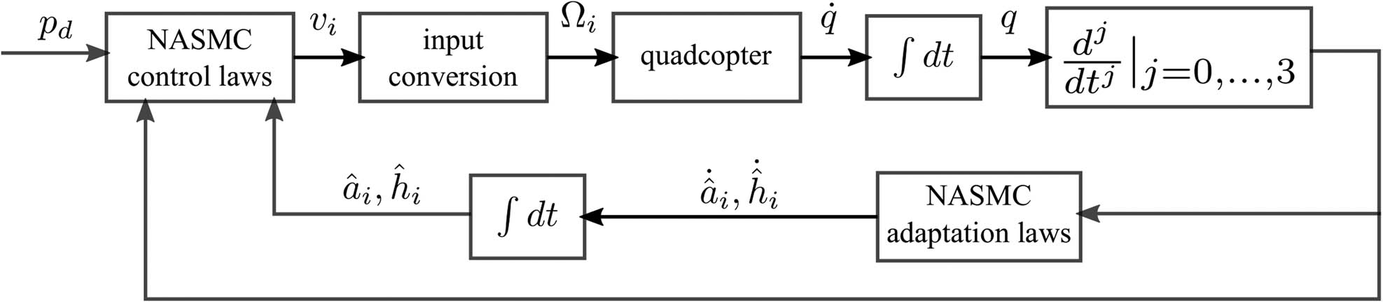
The control structure used in the simulation is presented in block diagram form in Figure 4. The computations needed to implement the controller are not complex. First, the desired motion is defined by the user as p d = [ x d , y d , z d , ψ d ] . Second, the block “NASMC control laws” (Eqs. (45), (46), (48), (50)) are calculated by receiving the state feedback q = [ r , v , Φ , ω ] and its derivatives from the quadcopter sensors (or a simulated quadcopter in Eqs. (26), (27), and (29)), and the estimated system parameters a ˆ i and h ˆ i . Third, the block “input conversion” (Eqs. (59) and (60)) calculates the rotor speeds. Finally, the rotor speeds are used to control the real quadcopter (or a simulated one using Eqs. (26), (27), (29)).

Figure 4

Control structure block diagram of quadcopter system.

At the same time, the state feedback q = [ r , v , Φ , ω ] and its derivatives from the quadcopter sensors (or a simulated quadcopter in Eqs. (26), (27), (29)) are used by the block “NASMC adaptation laws” (Eqs. (53), (54), (57), (58)) to calculate the system parameter correction rates. These rates are integrated and fed to the block “NASMC control laws.”

3.5 Computational complexity of the controller

As discussed in the previous section, the structure of the controller consists of four main blocks. The calculations involved in the NASMC approach are limited to the evaluation of four equations for the “NASMC control laws” block (Eqs. (45), (46), (48), and (50)), the evaluation of five equations in the “input conversion” block (Eqs. (59) and (60)), and the evaluation of 12 total equations in the “NASMC adaptation laws” block (Eqs. (53), (54), (57), and (58)). An additional computation overhead is needed to calculate the derivatives of the quadcopter states by the block marked d j d t j ∣ j = 0 , … , 3 in Figure 4. These calculations include the second and third derivatives of r x and r y , and the first derivative of ω vector. All other needed derivatives are provided by the real quadcopter sensors (or the quadcopter simulated model).

Next, these control subsystem equations are used in the quadcopter simulations as an example of the NASMC system. The simulation and results are presented in the next section.

4 Simulation

For the simulation that is shown as an example, a quadcopter is presented in a Simulink model. The quadcopter makes a great candidate use case for the NASMC approach, since it can take advantage of all the advantages that NASMC provides. Quadcopter users require the ability to use in many different environments, which have a high potential for unknown disturbances, because developing the dynamic system parameters is a difficult and costly endeavor. Furthermore, quadcopters also have a wide range of applications, from small camera drones all the way to large military operations vehicles. Groups that work with quadcopters are likely to use more than one system. Utilizing the NASMC scalability property requires no changes when implemented to other systems of similar type that use the same equations of motion but have different unknown parameters. All of these things are able to gain advantages from the use of the NASMC system, making the quadcopter a prime example for simulation and the use of this controller approach.

For our simulation to perform as we want it to, we must provide some assumptions and definitions that the controller can simulate. These are the desired motion functions, the gains used in the controllers, and the nominal values of the dynamic model parameters. These will be explained further.

4.1 The rationale for choosing the controller

There are two very important reasons for choosing a NASMC controller for any application. First, NASMC does not need prior knowledge of the dynamic system parameters. These dynamics system parameters are determined by extensive and time-consuming system identification experiment. Since NASMC does not require prior knowledge of the system parameters, its usage eliminates the extensive system identification experiments. Second, if the dynamic system parameters are changed due to the age of the system, NASMC approach adapts to the changed system parameters and maintains its performance even when the system ages.

4.2 Desired motion functions

The desired motion in our simulation would equate to the input of an operator who is piloting the quadcopter vehicle; however, we use a set of desired values in place of these operator inputs. The motion we choose to define is set by the following equations for the states:

x d = 0 if t ≤ 0.1 0.1 sin ( 2 π t / 100 ) if t > 0.1 y d = − x d z d = − 0.5 sin ( 2 π t / 200 ) ψ d = ( π / 4 ) sin ( 2 π t / 200 ) .

where the time derivatives are taken of these equations until the fourth derivatives for x d and y d and until the second derivatives for z d and ψ d . The position equations for all four states and all their time derivatives are provided as desired values. This desired path was chosen because the functions excite all DOFs, and they can be taken to the appropriate number of derivatives required by their respective subsystem.

4.3 Controller gains

For the v 2 and v 3 control subsystems that relate to x and y positions, we reference Eqs. (51) and (52), Eq. (3) with n = 4 for the fourth-order combined error, and Eqs. (53) and (54) for the adaptation laws. For the v 1 and v 4 control subsystems that relate to z and ψ , we reference Eqs. (55) and (56), Eq. (3) with n = 2 for the second-order combined error, and Eqs. (57), and (58) for the adaptation laws. Referencing these equations, we must define gains for each control subsystem, which can be found in Table 1.

Table 1

Controller gains for all four control subsystems for NASMC

	x	y	z	ψ
D i	0	0	0	0
η i	2	2	20	2
ϕ s i	0.05	0.05	0.05	0.05
λ i	2	2	3	1
γ i 0	21	21	100	100
γ i 1	100	100	100	100
γ i 2	100	100	—	100
γ i 3	100	100	—	—

The choice of gains was determined by experimentation. These gains are used in each control subsystem to fine-tune the abilities of the controllers. Note that all D values are set to zero. Since in each control law, D is only used in the context of ( D + η ) , the values selected for each η represent the sum of these two quantities. Results would be identical if the sum of each pair of D and η was equivalent to each η as currently defined.

4.4 Nominal values of dynamic model parameters

Contained within the dynamic model are many parameters, of which many are unknown to the controllers in the subsystems. These parameters are being adapted to by the subsystems and are used to give the dynamic model a nominal value, while the controllers output estimated values of h ˆ and a ˆ i , which contain these nominal values within. These parameters include d i , the distance from the geometric center of the quadcopter to each individual rotor, c T , the equivalent thrust coefficient, c Q , the torque coefficient, m , the mass, I , the mass moment of inertia matrix, and I x x y y , the average of I x x and I y y when needed because of the previous assumptions made in Section 3.3.1. These known nominal values are defined in Table 2 and the unknown nominal values are defined in Table 3. Note that we define m and I values as unknowns since they can change during the life of the quadcopter due to additions, modifications, damage, and more.

Table 2

Known nominal values of dynamic model parameters

d 1	0.226 m
d 2	0.226 m
d 3	0.226 m
d 4	0.226 m

Table 3

Unknown nominal values of dynamic model parameters

c T	7 × 1 0 − 6 kg m
c Q	2.6 × 1 0 − 7 kg m 2
m	1.138 kg
I x x	0.0077 kg m 2
I y y	0.0075 kg m 2
I z z	0.0127 kg m 2
I x x y y	0.0076 kg m 2

4.5 A benchmark controller for performance comparison

The non-adaptive counterpart of NASMC, which is simply named the Sliding Model Control (SMC), is commonly used for the control of nonlinear systems. The SMC method is very robust for systems with known parameters that have some bounded estimation errors. However, the SMC method cannot robustly control systems with completely unknown parameters. The proposed NASMC method in this article, can robustly control systems with unknown parameters.

To demonstrate the superiority of the NASMC approach to the plain SMC approach, both controllers are used on the same quadcopter in this section. However, at time 150 s of the simulation, the thrust coefficients c T and c Q are intentionally reduced to 60% of their original values. It is expected that the SMC method cannot adjust to this large and abrupt change of system parameters and will fail to control the quadcopter, whereas the NASMC can easily adjust to this abrupt system parameter change and successfully gain control of the quadcopter. The controller gains for the SMC approach are shown in Table 4.

Table 4

Controller gains for all four control subsystems for SMC

	x	y	z	ψ
D i	0	0	0	0
η i	2	2	20	2
ϕ s i	0.05	0.05	0.05	0.05
λ i	2	2	3	1

5 Results

This section includes the simulation results of the quadcopter model built in Simulink when provided the desired values, controller gains, and dynamic model parameters provided above. The simulation is run for 300 s to have a long time period to see the quadcopter tracking properly and for the parameters to have plenty of time to converge to their estimations. To demonstrate how the SMC and NASMC react to unknown parameter changes, at time 150 s of the simulation the thrust coefficients c T and c Q are intentionally reduced to 60% of their original values.

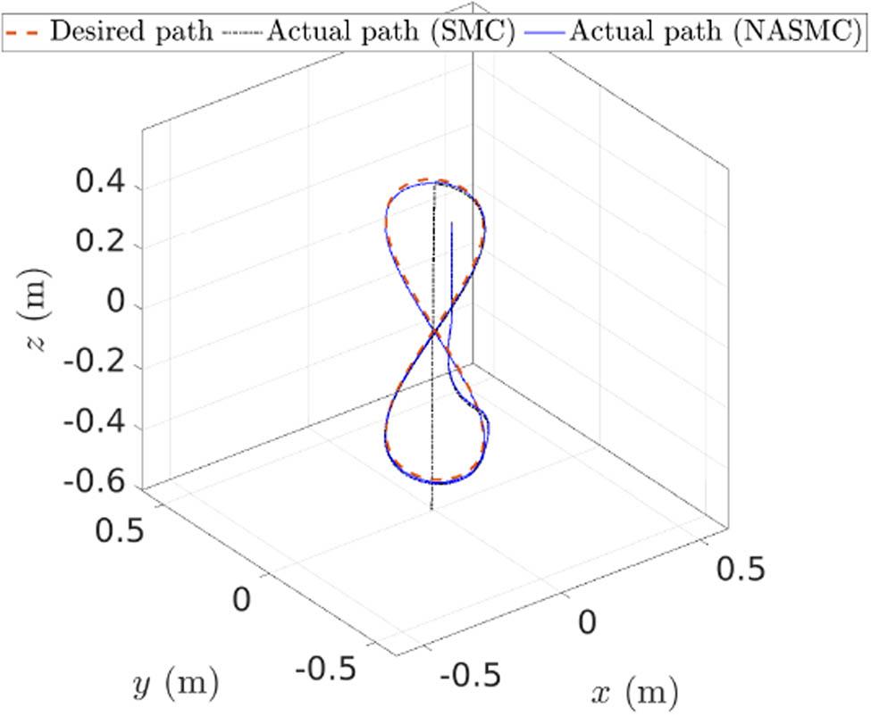
In Figure 5, we can see the actual 3D position path of the quadcopter compared to its desired position path. Figure 6 shows the tracking data of four states, x , y , z , and ψ . The quality of trajectory tracking can be established by studying these figures. A good tracking is indicated by an actual 3D position path overlapping with the desired position path.

Figure 5

3D position of the quadcopter system using SMC and NASMC.

Figure 6

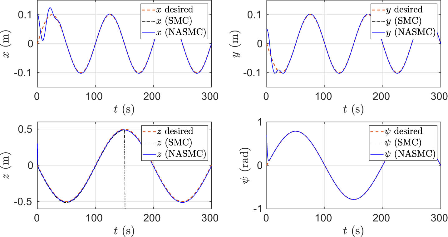
States tracking of the quadcopter system using SMC and NASMC.

Figure 7 shows the roll and pitch angle of the quadcopter. This provides further data on the orientation of the vehicle during simulation. A stable system would show small roll and pitch angles once settled.

Figure 7

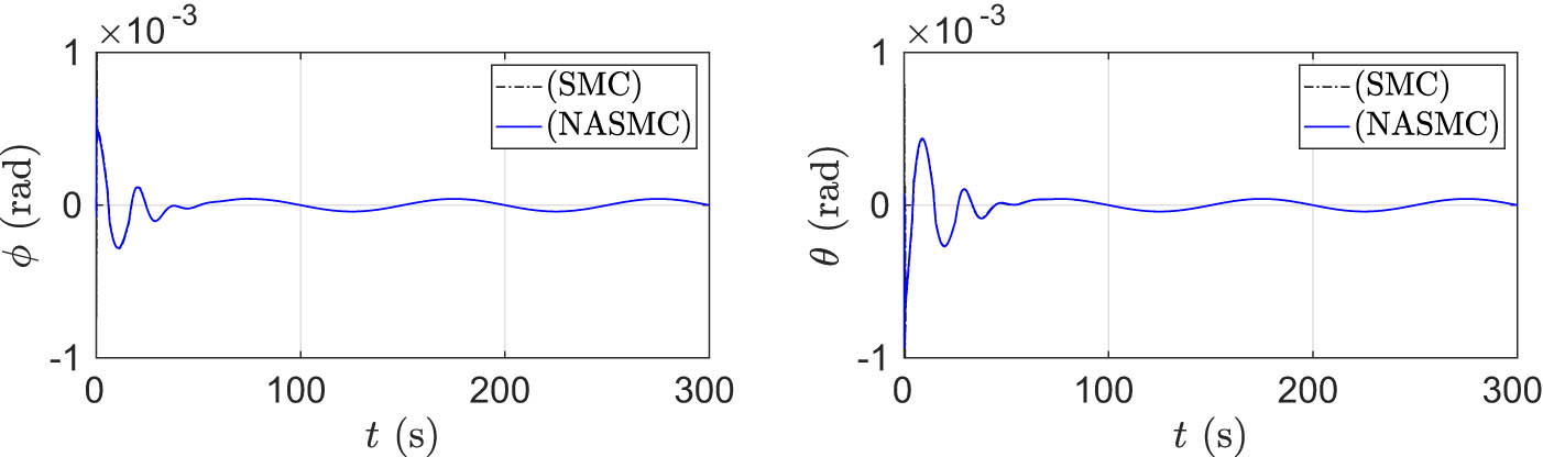
Roll and pitch angles of the quadcopter system using SMC and NASMC.

Figure 8 shows the individual rotor angular speeds during the simulation. This shows the data of the rotor speeds as they change while following the desired path. A stable system would show smooth changes in the angular speeds, since the desired path is smooth and slow.

Figure 8

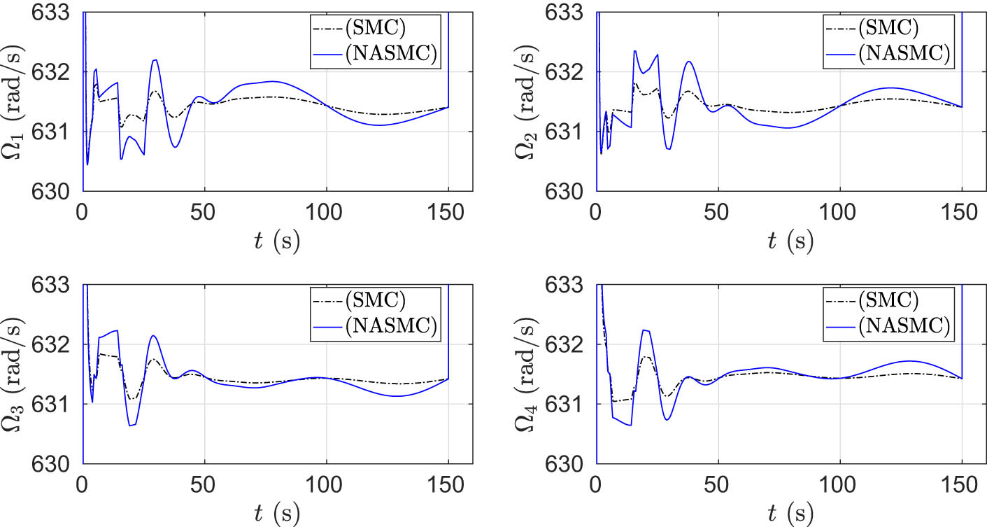
Rotor angular speeds of the quadcopter system using SMC and NASMC (the first 150 s of simulation).

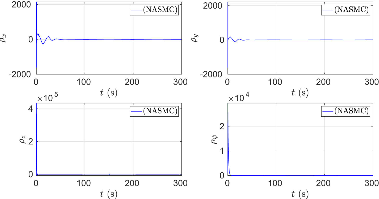
In Figure 9, we can see the residual error of the r x , r y , r z , and ψ states, respectively, as the simulation progresses. The remaining residual error for each state as time progresses can be determined with these figures. With good tracking, one would expect the residual error to approach zero.

Figure 9

Residual errors of quadcopter simulation using NASMC.

6 Discussion

By observing the results presented in Figures 5 and 6, one can see from the first glance that the tracking of the position path and the states very closely matches the desired values given after some time to stabilize the system to control for the unknown parameters. This shows that the NASMC is keeping the quadcopter controlled in a stable manner to match the desired results and that the actual position of the quadcopter vehicle never has a large deviation from the desired functions, even at time 150 s, when the rotors’ thrust coefficients are abruptly reduced to 60% of their original values. However, it can be seen that the z state of the quadcopter becomes unstable at 150 s when the nonadaptive SMC approach is used. The x and y states are physically stabilized by moments of all the four rotors’ thrust. Since the thrust of all the four rotors are reduced at the same time after the change in the rotors’ thrust coefficients at 150 s, the change in the controllability of the moment is negligible and the SMC can handle that negligible small change, and can still successfully control the x and y states.

Figure 7 continues to show the story of the stability of the NASMC. Even during the first section of the simulation when the control subsystems are still working to become stable, neither the roll nor pitch angle ever exceeds ± 1 × 1 0 − 3 rad, and only briefly before settling into a small amplitude sinusoidal pattern. There is no chaotic spike in the angles, and the NASMC system maintains stable control of the vehicle during the duration of the simulation length. Remember that the SMC can still successfully control the x and y states, which is why the roll and pitch are also still stabilized by the SMC.

Figures 8 and 10 show the angular speed of individual rotors for the first 150 s and for the last 150 s of the simulation, respectively. Referring to Figure 8, we see the angular speeds of each individual rotor on the vehicle as they change with time. The SMC and NASMC methods apply slightly different rotor speeds. Aside from some initial spikes at the start of the simulation, the vehicle quickly settles into a stable pattern of rotor speeds. 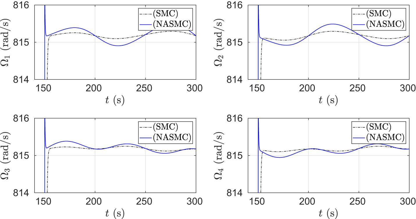As shown by the y -axis, the speed of all the rotors only varies a small amount once stable. This is due to the magnitude of the desired acceleration in the z direction being very low, with a peak of only ± 4.9348 × 1 0 − 4 m/s . This low acceleration leads to minimal variation in the rotor speeds and minimal change in total thrust. At time 150 s, both the SMC and NASMC methods react to the abrupt drop in the rotor’s thrust coefficients by increasing the rotor speeds.

Figure 10

Rotor angular speeds of the quadcopter system using SMC and NASMC (the second 150 s of simulations).

Referring to Figure 10, it can be seen that the NASMC adjusts the rotor speeds to the drop in rotors’ thrust coefficients to 60% of their original values at 150 s much faster than the SMC does. This fast adjustment is the key to the success of the NASMC to control the quadcopter despite the large parameter changes. By the time the SMC applies adjustments to rotor speeds, it has already lost control of the quadrotor in the z direction. Note that the convergence properties of the two SMC and NASMC are exactly the same, because they are using the same common gains (Tables 1 and 4). The only difference between the two is lack of adaptation for the SMC.

In Figure 9, we can see the tracking error dynamics for ρ x and ρ y driving close to zero by about 50 s into the simulation. This does take longer due to the nature of r x and r y being controlled by fourth-order subsystems. In Figure 9, we see ρ z and ρ ψ quickly driving to a very small residual error near zero. We can also see a very small spike at 150 s in ρ z . This is due to the application of the intentional sudden change in the thrust coefficients for testing at that time. The residual ρ z goes to zero very quickly after the small spike. Note that the order of magnitude of the peak of each of these residual errors is consistent with the corresponding nominal values of the parameters that appear in their definition. The parameters that appear in each residual error and their nominal values are listed in Table 5 with reference to their order of magnitude.

Table 5

Nominal unknown control parameters

ρ x	ρ y	ρ z	ρ ψ
h ˆ x = + 1,085	h ˆ y = + 1,085	h ˆ z = + 1.626 × 1 0 5	h ˆ ψ = 4.885 × 1 0 4
a ˆ x 1 = − 9,185	a ˆ y 1 = − 9,185	a ˆ z 1 = − 1.626 × 1 0 5	a ˆ 1 ψ = 0.769 × 1 0 4
a ˆ x 2 = + 8,900	a ˆ y 2 = + 8,900	a ˆ z 2 = 0	a ˆ 1 ψ = 4.885 × 1 0 4
a ˆ x 3 = − 1,085	a ˆ y 3 = − 1,085	—	—
a ˆ x 4 = 0	a ˆ y 4 = 0	—	—

7 Conclusion

The research in this article has demonstrated only a first glance at the potential capability of the NASMC approach. The quadcopter example shows its ability to adequately control the system when the parameters are unknown to the controller designer, removing the need for system identification experiments. All four states tracked closely with their corresponding desired values, roll and pitch angles along with all four rotor angular speeds all settled into a steady pattern, and all parameters quickly reached a steady state value that led to exponential convergence of s . This quadcopter model has shown effective implementation of the NASMC approach in a simulated environment. The tracking error is comparable to other control approaches for a quadcopter control (e.g., the nonadaptive SMC method) if the parameters of the system are known. However, the NASMC results have been achieved while the controller is unaware of system parameters, a feature unmatched by other approaches. In fact, it is shown that NASMC adjusts to abrupt parameter changes in the system, while SMC fails in that scenario. The second-order and fourth-order system derivations have been presented here and used in the example, but the NASMC will function similarly with any nth-ordered system by following the same methods shown here.

The successful simulation of NASMC with the quadcopter shows its strong potential for continued future development, research, and experimentation to build upon the research presented in this article. As long as researchers or control engineers can write the governing differential equations of their dynamic system in the form of Eq. (1), they can use the proposed controller. Examples of systems whose governing differential equations can be written in the form of Eq. (1) are robotic arms, spacecraft, airplanes, etc. Exploring the application of NASMC on robotic arms, spacecraft, airplanes, etc. can be considered as further development opportunity.

Funding information: This research was not funded by any funding agency.
Author contributions: The research idea and the overall methodology were formulated by F.F. The detailed derivations of the approach and the creation of the computer simulation code were performed by R.M., with suggested corrections in the derivations and some code debugging and additions by F.F. The draft manuscript was authored by R.M., which went through several revisions according to feedback from F.F. All authors have accepted responsibility for the entire content of this manuscript and approved its submission. The first author was a graduate student who conducted this research as required by his Master’s of Science thesis. The second author was the first author s thesis research advisor.
Conflict of interest: The authors state that there is no conflict of interest.

References

[1] Bangura M, Mahony RE. Nonlinear dynamic modeling for high performance control of a quadrotor. Australasian Conference on Robotics and Automation; 2012 Dec 3–5; Wellington, New Zealand. Curran Associates, Inc., 2014. p. 115–25. Search in Google Scholar

[2] Mahony RE, Kumar VR, Corke P. Multirotor aerial vehicles: modeling, estimation, and control of quadrotor. IEEE Robotic Autom Magazine. 2012;19(3):20–32. 10.1109/MRA.2012.2206474Search in Google Scholar

[3] Hua MD, Hamel T, Morin P, Samson C. Introduction to feedback control of underactuated VTOLvehicles: A review of basic control design ideas and principles. IEEE Control Syst Magazine. 2013;33(1):61–75. 10.1109/MCS.2012.2225931Search in Google Scholar

[4] Bouabdallah S, Siegwart RY. Full control of a quadrotor. 2007 IEEE/RSJ International Conference on Intelligent Robots and Systems; 2007 29 Oct–2 Nov; San Diego (CA), USA. IEEE, 2007. p. 153–8. 10.1109/IROS.2007.4399042Search in Google Scholar

[5] Mian AA, Daobo W. Nonlinear Flight control strategy for an underactuated quadrotor aerial robot. 2008 IEEE International Conference on Networking, Sensing and Control; 2008 Apr 6–8; Sanya, China. IEEE, 2008. p. 938–42. 10.1109/ICNSC.2008.4525351Search in Google Scholar

[6] Abdessameud A, Tayebi A. Global trajectory tracking control of VTOL-UAVs without linear velocity measurements. Automatica. 2010;46(6):1053–9. 10.1016/j.automatica.2010.03.010Search in Google Scholar

[7] Choi YC, Ahn H. Nonlinear control of quadrotor for point tracking: actual implementation and experimental tests. IEEE/ASME Trans Mechatr. 2015;20(3):1179–92. 10.1109/TMECH.2014.2329945Search in Google Scholar

[8] Yu Y, Guo Y, Pan X, Sun C. Robust backstepping tracking control of uncertain MIMO nonlinear systems with application to quadrotor UAVs. 2015 IEEE International Conference on Information and Automation; 2015 Aug 8–10; Lijiang, China. IEEE, 2015. p. 2868–73. 10.1109/ICInfA.2015.7279776Search in Google Scholar

[9] Hua MD, Hamel T, Morin P, Samson C. A control approach for thrust-propelled underactuated vehicles and its application to VTOL drones. IEEE Trans Automatic Control. 2009;54(8):1837–53. 10.1109/TAC.2009.2024569Search in Google Scholar

[10] Yesildirek A, Imran B. Nonlinear control of quadrotor using multi Lyapunov functions. 2014 American Control Conference; 2014 Jun 4–6; Portland (OR), USA. IEEE, 2014. p. 3844–9. Search in Google Scholar

[11] Adigbli P, Grand C, Mouret JB, Doncieux S. Nonlinear attitude and position control of a micro quadrotor using sliding mode and backstepping techniques. 3rd US-European Competition and Workshop on Micro Air Vehicle Systems (MAV07) & European Micro Air Vehicle Conference and Flight Competition (EMAV2007); 2007 Sep 18–22; Toulouse, France. IMAV, 2007. p. 17–21. Search in Google Scholar

[12] Xu R, Özgüner Ü. Sliding mode control of a class of underactuated systems. Automatica. 2008;44(1):233–41. 10.1016/j.automatica.2007.05.014Search in Google Scholar

[13] Runcharoon K, Srichatrapimuk V. Sliding mode control of quadrotor. 2013 The International Conference on Technological Advances in Electrical, Electronics and Computer Engineering (TAEECE); 2013 May 9–11; Konya, Turkey. IEEE, 2013. p. 552–7. 10.1109/TAEECE.2013.6557334Search in Google Scholar

[14] Chengshun Y, Yang Z, Huang X, Li S, Zhang Q. Modeling and robust trajectory tracking control for a novel six-rotor unmanned aerial vehicle. Math Problems Eng. 2013;2013(1):1–13. Search in Google Scholar

[15] Lee T, Leok M, Mcclamroch NH. Geometric tracking control of a quadrotor UAV on SE(3). IEEE Conference on Decision and Control; 2010 Dec 15–17; Atlanta (GA), USA. IEEE, 2011. p. 5420–5. 10.1109/CDC.2010.5717652Search in Google Scholar

[16] Roberts A, Tayebi A. Adaptive position tracking of VTOL UAVs. IEEE Trans Robotics. 2010;27(1):129–42. 10.1109/CDC.2009.5400947Search in Google Scholar

[17] Lee T, Leok M, McClamroch NH. Nonlinear robust tracking control of a quadrotor UAV on SE(3). Asian J Control. 2013;15(2):391–408. 10.1002/asjc.567Search in Google Scholar

[18] Lee T. Robust adaptive attitude tracking on SO(3) with an application to a quadrotor UAV. IEEE Trans Control Syst Tech. 2013;21(5):1924–30. 10.1109/TCST.2012.2209887Search in Google Scholar

[19] Zhao B, Xian B, Zhang Y, Zhang X. Nonlinear robust adaptive tracking control of a quadrotor UAV via immersion and invariance methodology. IEEE Trans Industr Electr. 2015;62(5):2891–902. 10.1109/TIE.2014.2364982Search in Google Scholar

[20] Kayacan E, Maslim R. Type-2 fuzzy logic trajectory tracking control of quadrotor VTOL aircraft with elliptic membership functions. IEEE/ASME Trans Mechatr. 2017;22(1):339–48. 10.1109/TMECH.2016.2614672Search in Google Scholar

[21] Zheng EH, Xiong JJ, Luo JL. Second order sliding mode control for a quadrotor UAV. ISA Trans. 2014;53(4):1350–6. 10.1016/j.isatra.2014.03.010Search in Google Scholar PubMed

[22] Tayebi A, McGilvray S. Attitude stabilization of a VTOL quadrotor aircraft. IEEE Trans Control Syst Technol. 2006;14(3):562–71. 10.1109/TCST.2006.872519Search in Google Scholar

[23] Mellinger D, Michael N, Kumar V. Trajectory generation and control for precise aggressive maneuvers with quadrotors. Int J Robotic Res. 2012;31(5):664–74. 10.1007/978-3-642-28572-1_25Search in Google Scholar

[24] Yu Y, Ding X. A Global tracking controller for underactuated aerial vehicles: design, analysis, and experimental tests on quadrotor. IEEE/ASME Trans Mechatr. 2016;21(5):2499–511. 10.1109/TMECH.2016.2558678Search in Google Scholar

[25] Poultney A, Kennedy C, Clayton GM, Ashrafiuon H. Robust tracking control of quadrotors based on differential flatness: simulations and experiments. IEEE/ASME Trans Mechatr. 2018;23(3):1126–37. 10.1109/TMECH.2018.2820426Search in Google Scholar

[26] Slotine JJE, Li W. Applied nonlinear control. Upper Saddle River (NJ), USA: Prentice Hall; 1991. Search in Google Scholar

[27] Slotine JJE, Coetsee J. Adaptive sliding controller synthesis for non-linear systems. Int J Control. 1986;43(6):1631–51. 10.1080/00207178608933564Search in Google Scholar

Received: 2022-08-10

Revised: 2022-10-26

Accepted: 2022-11-29

Published Online: 2023-02-28

This work is licensed under the Creative Commons Attribution 4.0 International License.

Articles in the same Issue

https://doi.org/10.1515/nleng-2022-0268

Keywords for this article

nonlinear control; nth-order adaptive variable structure control; fourth-order quadcopter model; single-loop quadcopter control; unknown system parameters

Creative Commons

BY 4.0