Dynamical structures of wave front to the fractional generalized equal width-Burgers model via two analytic schemes: Effects of parameters and fractionality
-
Mst. Razia Pervin
 ,
Alrazi Abdeljabbar
,
Pinakee Dey
,
Alrazi Abdeljabbar
,
Pinakee Dey

Abstract
This work focuses on the fractional general equal width-Burger model, which describes one-dimensional wave transmission in nonlinear Kerr media with combined dispersive and dissipative effects. The unified and a novel form of the modified Kudryashov approaches are employed in this study to investigate various analytical wave solutions of the model, considering different powers of nonlinearity in the Kerr media. As a result, a wide range of structural solutions, including trigonometric, hyperbolic, rational, and logarithmic functions, are formulated. The achieved solutions present a kink wave, a collision of kink and periodic peaked soliton, exponentially increasing wave profiles, and shock with a dark peaked wave. The obtained solutions are numerically demonstrated for specific parameter values and general parametric powers of nonlinearity. We analyzed the effect of existing parameters on the obtained wave solutions with numerical graphics. Moreover, the stability of the model is analyzed with a perturbed system. Furthermore, a comparison with published results in the literature is provided, highlighting the differences and similarities. The achieved results showcase the diversity of structural solutions obtained through the proposed approaches.
1 Introduction
Nonlinear fractional evolution models have emerged as powerful tools for modeling various phenomena in science and engineering, particularly in the context of miniature, sensitive, and microscopic systems [1,2,3]. These models have found applications in capturing complex physical states [4,5,6] and are instrumental in accurate modeling of intricate nonlinear phenomena. In the existing literature, different types of fractional models have been proposed to facilitate precise modeling. Examples include the Jumarie Riemann–Liouville (JRL) fractional model [7,8], modified Riemann–Liouville fractional model [9,10], conformable time-fractional model [11,12], fractional beta model [13,14], M-fractional model [15], and many others. Among these fractional models, the JRL fractional model satisfies most of the desirable properties of differentiation, while other models may exhibit some undesirable or anomalous behaviors. In light of this, the present write-up focuses on the spatial-temporal fractional general equal width (GEW)-Burgers model in the framework of the JRL fractional sense. The model is represented as follows:
where D α and D β denote the JRL fractional derivatives, and α, β, and m are real constant parameters. The GEW-Burgers model incorporates fractional order derivatives with respect to both space and time variables, and the novel fractional JRL derivative is employed for precise characterization.
Only a limited number of researchers have investigated the GEW-Burgers equation using analytical techniques. Nuruddeen and Nass [15] employed the Kudryashov technique to extract exact solitary wave solutions for both the classical and fractional derivative versions of the model. Hamdi et al. [16] derived a few exact results for the model using only the classical derivative. Research on this model is scarce, yet it holds significant applications in wave transmission within nonlinear media, encompassing both dispersive and dissipative effects. Notably, GEW-Burger has been studied solely in the context of the conformable fractional case [15].
This research aims to modify the model into the form given in Eq. (1) using the JRL fractional sense. The key question now pertains to identifying appropriate techniques for exploring the intricate dynamics arising from integrating our proposed fractional nonlinear model (1). Various techniques have been employed in recent works to obtain exact solutions for fractional partial differential equations, ranging from semi-analytical schemes to unified procedures [17,18,19,20,21,22,23,24,25,26,27,28,29,30,31,32,33,34]. Among them, the unified technique stands out due to its incorporation of tanh and exp-functions approaches.
In this write-up, we shed light on the use of the Unified method [32,33,34] to analytically investigate the fractional GEW-Burgers model. In addition, a novel form of the modified Kudryashov (NFMK) [35] scheme enables the discovery of innovative arbitrary number base wave solutions.
The structure of this write-up is as follows: Section 2 provides elementary definitions and properties of JRL fractional derivatives. Integral techniques are briefly explained in Section 3. In Section 4, we extract novel solutions of the space-time fractional generalised equal width-Burgers model using the unified and NFMK techniques. The results are presented in Section 5, followed by a comparison with other results in Section 6. Finally, the write-up concludes with a summary in Section 7.
2 Properties of JRL derivative
In this section, we compile essential properties and notes related to the definition of
The
where
Some significant properties are as follows:
For others properties see [8].
3 Methodology
This segment represents fractional unified and NFMK schemes as well as their applications to the space–time JRL fractional GEW–Burger model to accomplish new solutions.
3.1 Basic information of fractional unified scheme
This section illustrates fractional unified scheme [32,33,34] for guiding analytical solutions to nonlinear fractional evolution equations (NFEEs) in a succeeding manner. Consider an NFEE in independent variables
where
Step 1: Converting the NFEE into ordinary differential equation (ODE) with the advantages of operating wave mapping
where
Step 2: Now Eq. (5) can be integrated requisite times with integral constant as zero.
Consider that Eq. (5) has a series solution as follows:
where
which has results as:
Case 1: On condition
Case 2: On
where
Case 3: On
Step 3: Using Eq. (7), the value of
3.2 Basic phases of NFMK technique
The trial result of Eq. (5) in the ensuing form is
where
where
To develop unknown constants, Eq. (11) into Eq. (4) combining use of Eqs (12) and (13). Formerly, transform to a polynomial of
The integrated result of Eq. (13) is
Remark: Our new modified Kudryashov’s (MK) technique familiarized result in terms of a series
4 Integrate the fGEW-Burgers model to extraction solutions
Recall space–time JRL fractional GEW-Burgers model (Eq. (1)) as well as assembling the wave transformation
Eq. (1) turned to an ODE,
By integrating Eq. (15) once, as well as bearing in mind integral constant as zero, attains
Evaluating balance from highest derivatives with the nonlinear term
Incorporating the mapping
The next sub-steps are going to exploit wave solutions through the fractional unified and NFMK techniques.
4.1 Solutions by fractional unified technique
Balancing the highest derivatives and nonlinear term (i.e.,
The following algebraic equations, by replacing Eq. (18) into Eq. (17) as well as putting every coefficient of
Solving the above systems of Eq. (19), one obtains the succeeding results:
Set 1:
The following general solutions of Eq. (1) can be found by Set 1 and combining Eqs (8), (9), (10), and (18):
For
For
For
where
Set 2:
The following general results of Eq. (11) are found by using Set 2 and combining Eqs (8), (9), (10), and (15):
For
For
For
where
Set 3:
Other solutions can be written in a similar manner due to Set 3 as well as combining Eqs (8), (9), (10), and (15). Few are as follows:
4.2 Solutions by NFMK technique
Subsequently, due to the balance number
with
Differentiating Eq. (20) sufficient times and taking advantage of Eq. (11) yields a class of equations whose solutions are as follows:
These two constraints afford new categorical wave solutions that are
where
where
5 Results and discussions
This section explained the numerical representation of the obtained solution through the unified and NFMK techniques.
5.1 Numerical illustration of solutions by unified technique
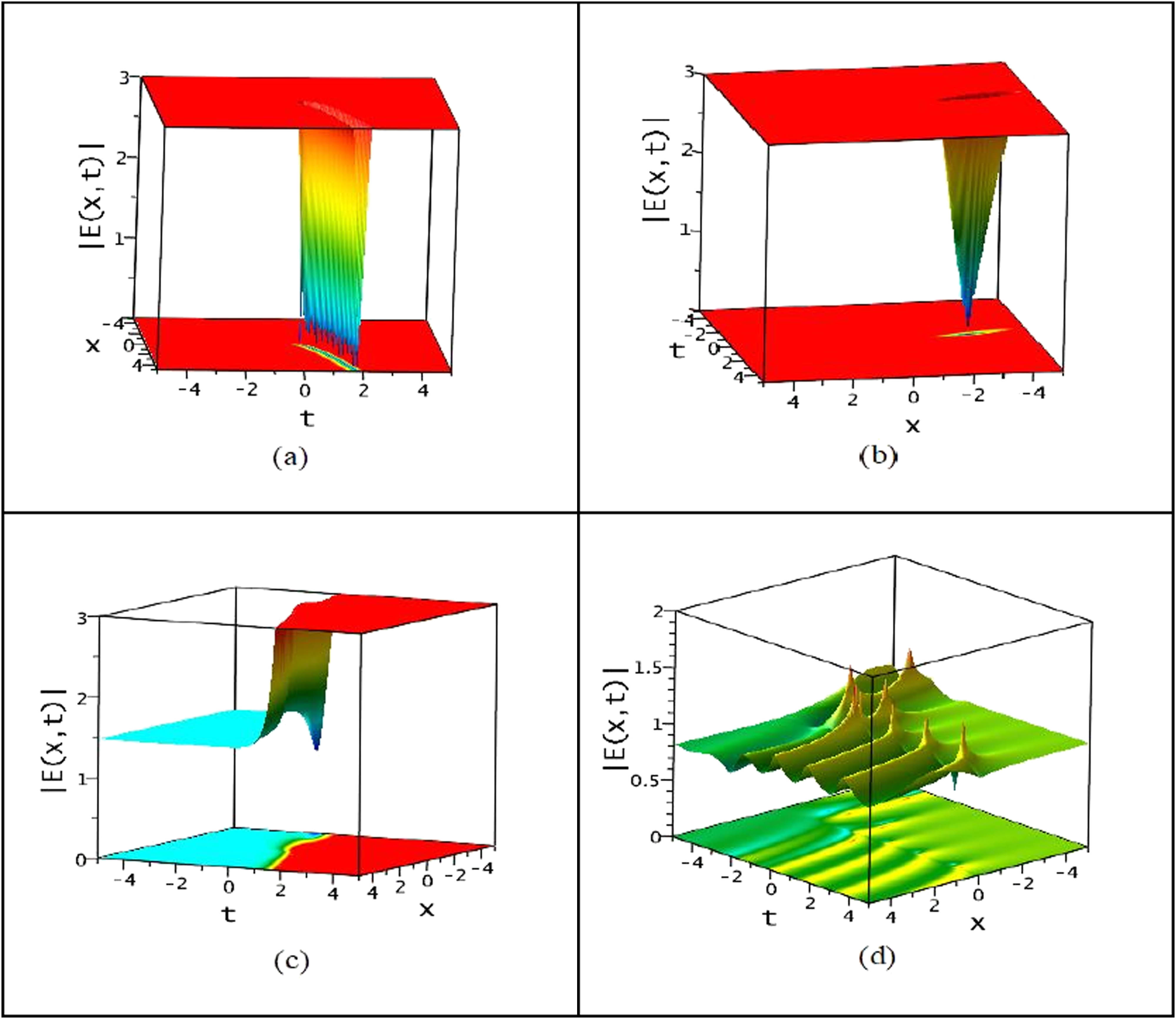
All the solutions are achieved by the unified scheme in terms of trigonometric, hyperbolic, and rational functions that presented periodic, solitonic, and singular solitonic behaviors, respectively, with general parametric power nonlinearity. Actually, 54 solutions by the set of constraints are gathered here. Various distinct behaviors are illustrated with regard to particular values of free parameters in 3-D, 2-D, and contour plots. In Figure 1: shock-like wave
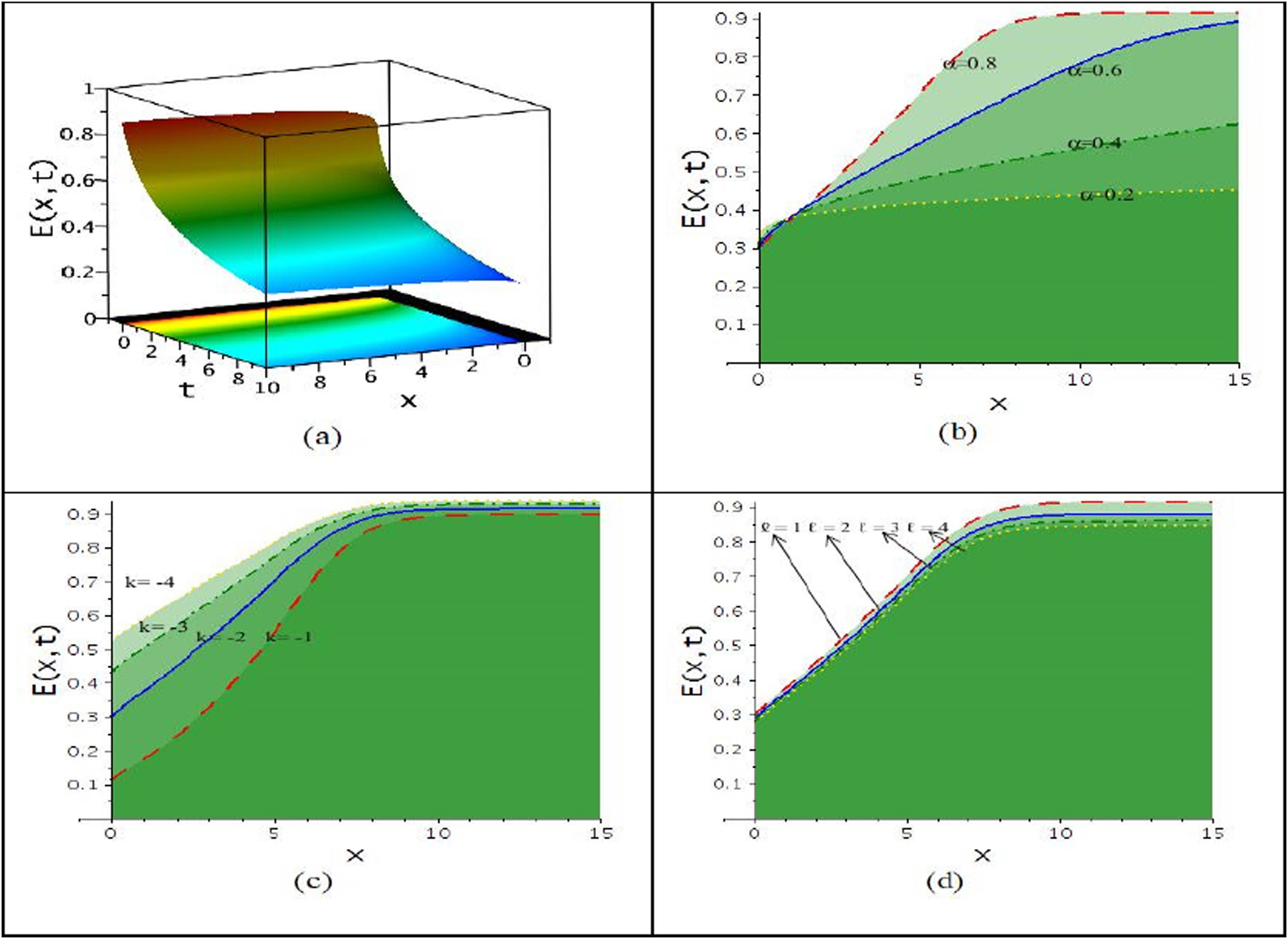
Shock wave solution via
Modulation of shock-peaked wave solution
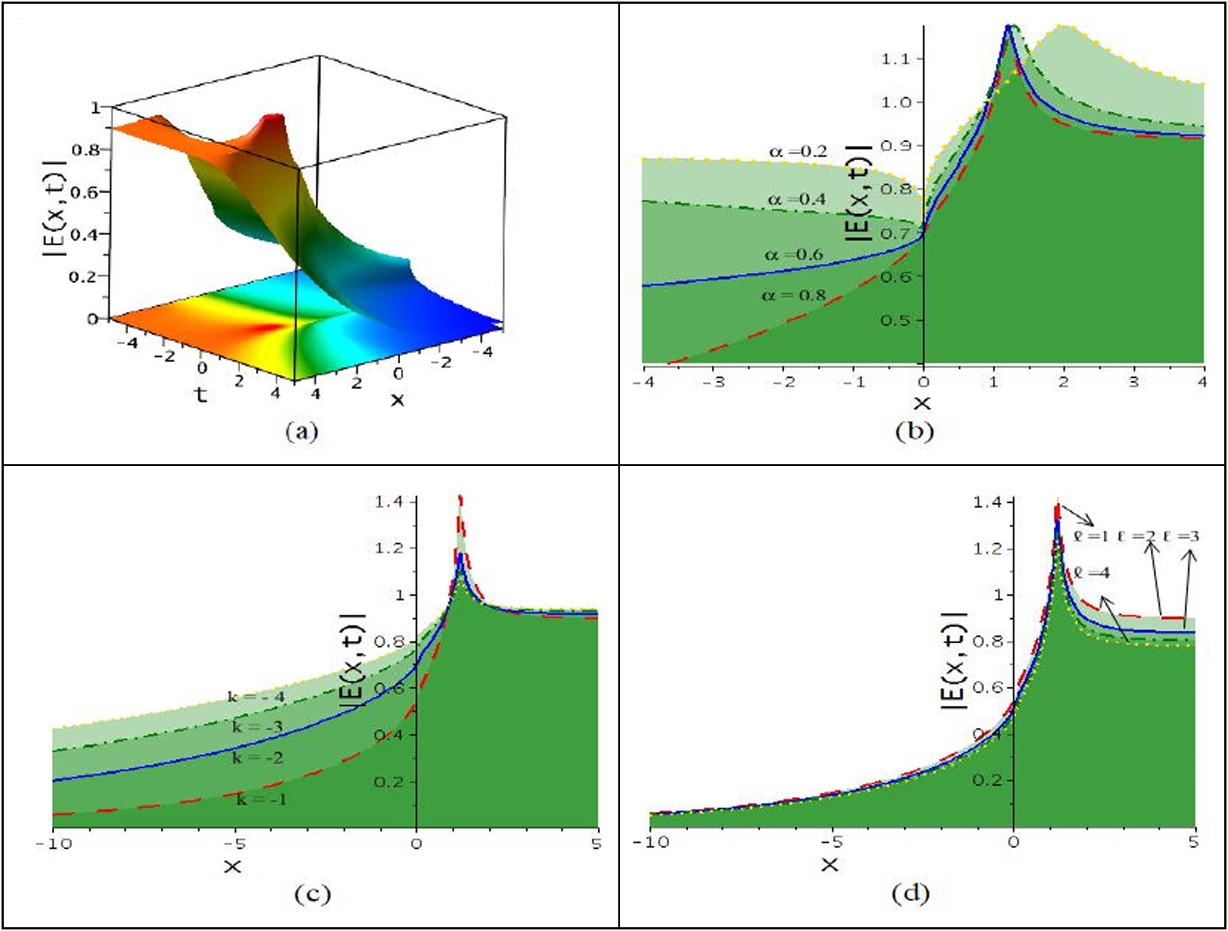
In Figure 3: modulus plots of periodic wave is depicted via
Modulation of periodic wave solution
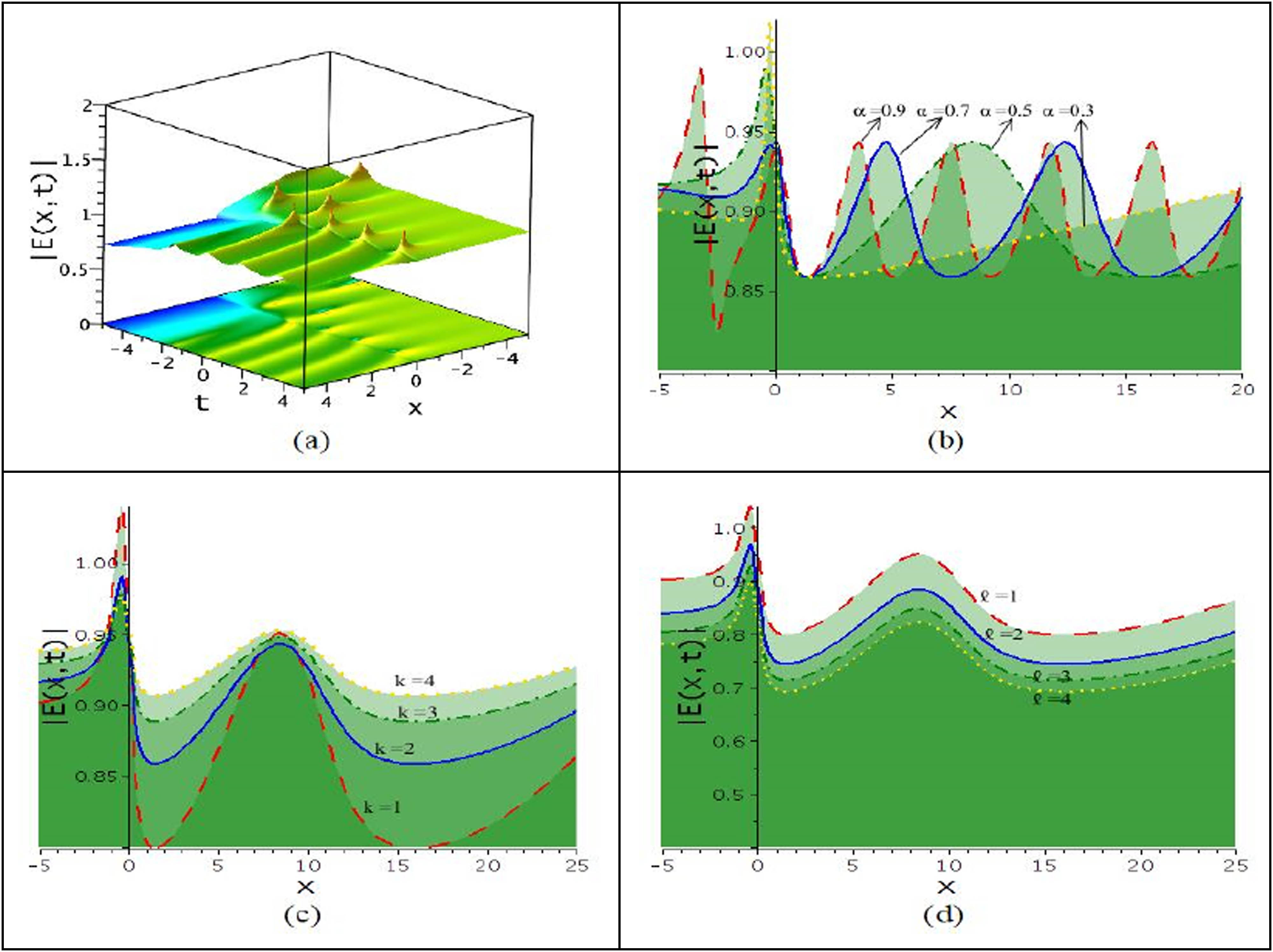
Wave solutions with 3D (upper) as well as contour (below) plots as (a)
In Figure 5, the modulation wave solution (from Set-3) presents dark peaked wave taking with
5.2 Numerical illustration of solutions by NFMK technique
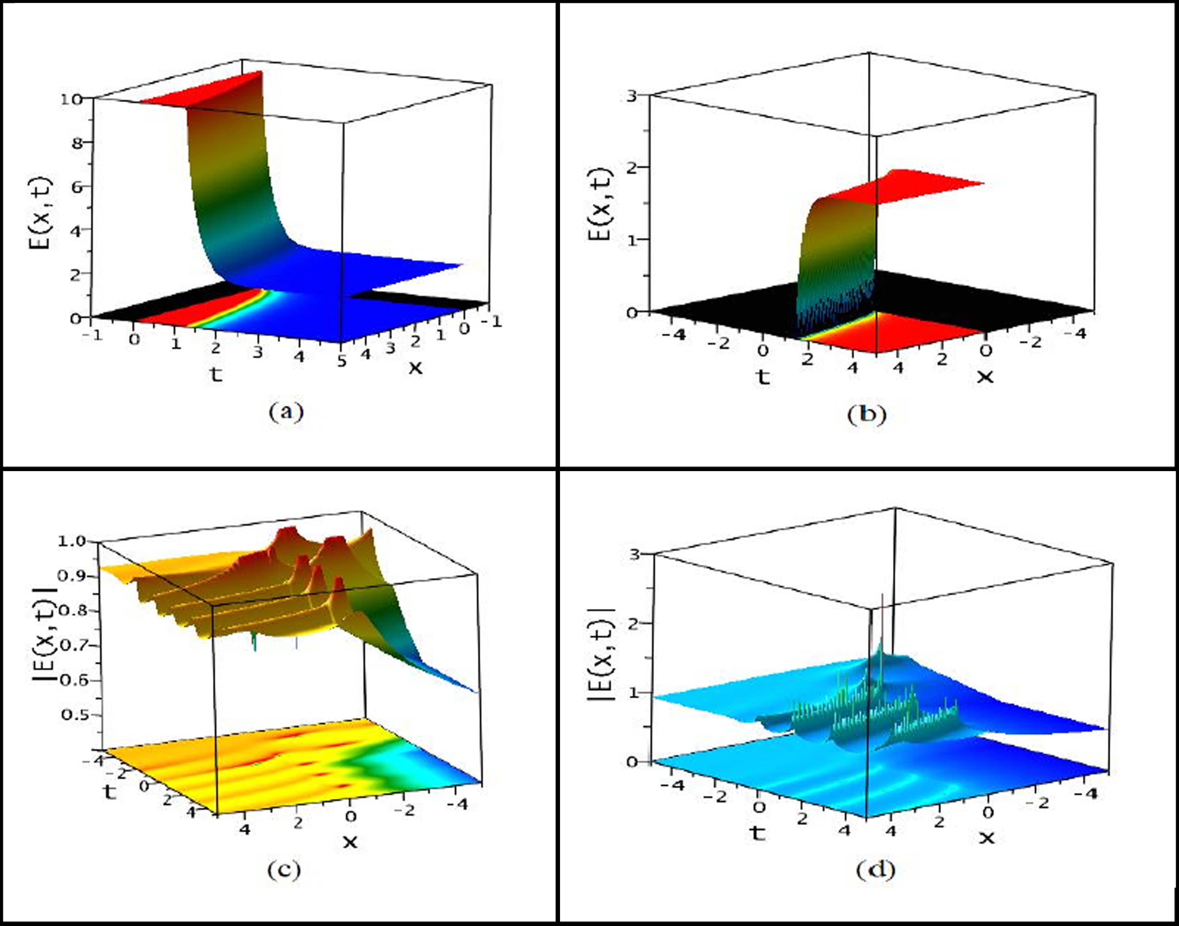
This NFMK scheme extracted only two solutions on the basis of arbitrary parameters. Due to the change of values, it illustrated various appeals in a diverse wave pattern. Few are expressed with particular numerical values. The increasing and decreasing of wave height for change in parameters and fractionality are presented in Figure 6 for
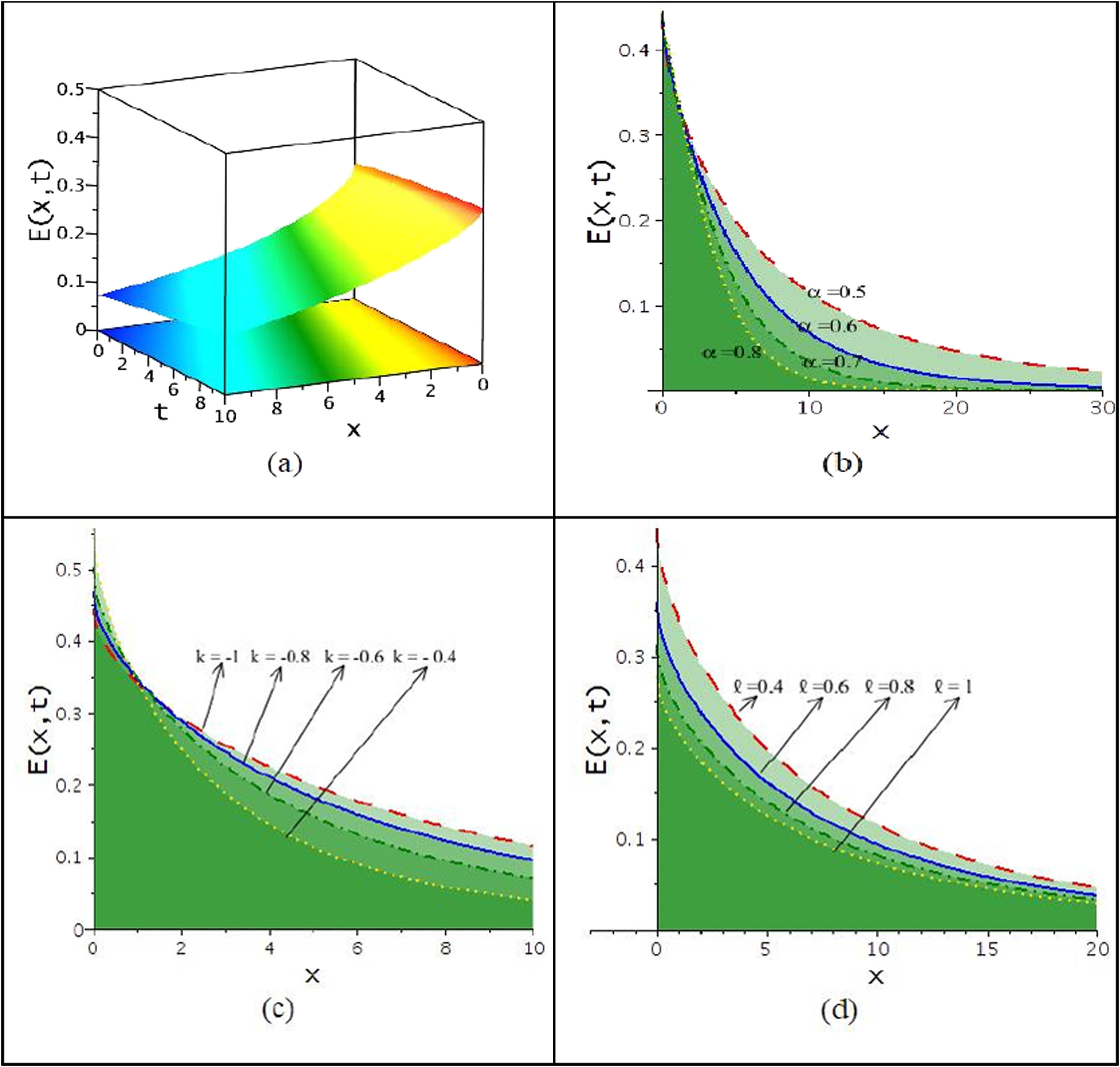
Modulation shock-peaked wave solution: (a) 3D (upper) and contour (lower) plots, (b) effects of fractionality due to changes of

Modulation shock-peaked wave solution: (a) 3D (upper) and contour (lower) plots, (b) effects of fractionality due to changes of
6 Stability analysis
In this fragment, we have derived the conditions of stability of model (1) and doing so let us consider the perturbed solution
where
Applying (21) into Eq. (1), convert to the form
Linearizing the above equation, we have
Again setting
where
The transmission relationships of Eq. (23) are observed here. The sign of
7 Comparison
In comparison with the results of [15,16], this research enriches the study of fractionality, general parametric power nonlinear solutions, and a variety of nonlinear structural wave fronts for the GEW-Burger equation. Nuruddeen and Nass [15] studied the classical and conformable fractional forms of the equation using the Kudryashov scheme, obtaining only one solution in the exponential function. Similarly, Hamdi et al. [16] found only one solitary wave solution for the classical GEW-Burger model, which is weaker than the result by Nuruddeen and Nass [15] (see comparison section of [15]).
In contrast, our research modifies the model in the form of Eq. (1) with the JRL fractional sense, which is considered more reliable than the conformable fractional derivative. The fractional GEW-Burger model is integrated using the unified and NFMK techniques, which encompass all solutions obtained by Nuruddeen and Nass and Hamdi et al. [15,16]. As a result, we achieve a vast multiplicity of solutions in terms of rational, periodic, and hyperbolic forms. Additionally, we discuss the effects of each parameter, fractionality, and general parametric power nonlinearities on the obtained results.
8 Conclusion and future works
In conclusion, this research successfully integrated the space-time JRL fractional GEW-Burgers equation using the powerful Unified and NFMK schemes. The study yielded a wide array of solutions for this model with a general parametric power nonlinearity. A comprehensive comparison was made between the results obtained in this study and those from the usual GEW-Burgers model in [15]. To aid in the comparison, 3-D graphical illustrations for specific solutions and 2-D shapes (refer to Figures 1–7) were provided, showcasing changes in nonlinearity and parameters. Furthermore, the impact of dispersion, dissipation, and general parametric power nonlinearity on wave height was observed and depicted through 3D, 2D, and contour plots (see Figures 1–7). The stability analysis is also performed for the considered model. The methods used in this research have several notable advantages. Firstly, they are highly versatile, enabling the discovery of solitary and periodic wave solutions with great simplicity. Secondly, exact solutions were obtained by considering various functions, making these techniques highly recommended for both general and non-general problems.
Looking ahead, our future task involves exploring the interaction of solitons, rogue waves, and bullet solitons. Additionally, the model can be further modified in M-fractional form and two-mode form to extend its applicability to different scenarios [36 37 38 39].
Acknowledgments
Thanks to the editor, reviewers, and Khalifa University, Abu Dhabi, United Arab Emirates, for technical support of the research.
-
Funding information: This research has external funding from Khalifa University, United Arab Emirates.
-
Author contributions: Methodology, software, writing – original draft, M.R. Pervin; conceptualization, software, writing – original draft, H.-O.-R.; supervision, validation, and data curation, A.A. (P. Dey); supervision, corrections and validation (S.S. Shanta); checking draft, validation, A.A. (Alrazi Abdeljabbar). All authors have read and agreed to publish this version of the manuscript.
-
Conflict of interest: The authors affirm that they have no known competing financial interests or personal relationships that could have seemed to influence the work reported in this paper.
-
Data availability statement: The manuscript has no associated data.
References
[1] Khalil R, Al Horani M, Yousef A, Sababheh M. A new definition of fractional derivative. J Comput Appl Math. 2014;264:65–70.10.1016/j.cam.2014.01.002Search in Google Scholar
[2] Yang Y. The fractional residual method for solving the local fractional differential equations. Therm Sci. 2020;24(4):2535–42.10.2298/TSCI2004535YSearch in Google Scholar
[3] Kilbas AA, Srivastava HM, Trujillo JJ. Theory and applications of fractional differential equations. North-Holland Mathematics Studies. Vol. 204. 2006.Search in Google Scholar
[4] Islam Z, Abdeljabbar A, Sheikh Md, Roshid HO, Taher MA. Optical solitons to the fractional order nonlinear complex model for wave packet envelope. Results Phys. 2022;43:106095. 10.1016/j.rinp.2022.106095.Search in Google Scholar
[5] Abdeljabbar A, Roshid HO, Aldurayhim A. A bright, dark, and rogue wave soliton solutions of the quadratic nonlinear Klein–Gordon equation. Symmetry. 2022;14:1223. 10.3390/sym14061223.Search in Google Scholar
[6] Osman M, Ghanbari B. New optical solitary wave solutions of Fokas-Lenells equation in presence of perturbation terms by a novel approach. Optik. 2018;175:328–33.10.1016/j.ijleo.2018.08.007Search in Google Scholar
[7] Guo M, Fu C, Zhang Y, Liu J, Yang H. Study of ion-acoustic solitary waves in a magnetized plasma using the three-dimensional time-space fractional Schamel-KdV equation. Complexity. 2018;2018:6852548.10.1155/2018/6852548Search in Google Scholar
[8] Jumarie G. Modified Riemann-Liouville derivative and fractional Taylor series of non-differentiable functions further results. Comput Math Appl. 2006;51:1367–76.10.1016/j.camwa.2006.02.001Search in Google Scholar
[9] Jumarie G. Table of some basic fractional calculus formulae derived from a modified Riemann-Liouville derivative for non-differentiable functions. Appl Math Lett. 2009;22:378–85.10.1016/j.aml.2008.06.003Search in Google Scholar
[10] Nisar KS, Akinyemi L, Inc M, Şenol M, Mirzazadeh M, Houwe A, et al. New perturbed conformable Boussinesq-like equation: Soliton and other solutions. Results Phys. 2022;33:105200.10.1016/j.rinp.2022.105200Search in Google Scholar
[11] Eslami M, Rezazadeh H. The first integral method for Wu–Zhang system with conformable time-fractional derivative. Calcolo. 2015;53:475.10.1007/s10092-015-0158-8Search in Google Scholar
[12] Hosseini K, Kaur L, Mirzazadeh M, Baskonus HM. 1-soliton solutions of the (2 + 1)-dimensional Heisenberg ferromagnetic spin chain model with the beta time derivative. Opt Quant Electron. 2021;53:125.10.1007/s11082-021-02739-9Search in Google Scholar
[13] Rahman Z, Abdeljabbar A, Roshid HO, Ali MZ. Novel precise solitary wave solutions of two time fractional nonlinear evolution models via the MSE scheme. Fractal Fract. 2022;6:444. 10.3390/fractalfract6080444.Search in Google Scholar
[14] Rahman Z, Ali MZ, Roshid HO. Closed form soliton solutions of three nonlinear fractional models through a proposed Improved Kudryashov method. Chin Phys B. 2021;30:050202.10.1088/1674-1056/abd165Search in Google Scholar
[15] Nuruddeen RI, Nass MA. Exact solitary wave solution for the fractional and classical GEW-Burgers equations: an application of Kudryashov method. J Taibah Univ Sci. 2018;12(3):309–14. 10.1080/16583655.2018.1469283.Search in Google Scholar
[16] Hamdi S, Enright WH, Schiesser WE, Gottlieb JJ. Exact solutions of the generalized equal width equation. Comp Sci Appl. 2003;2668:725–34.10.1007/3-540-44843-8_79Search in Google Scholar
[17] Yusuf A, Sulaiman T, Abdeljabbar A, Alquran M. Breather waves, analytical solutions and conservation laws using Lie–Bäcklund symmetries to the (2 + 1)-dimensional Chaffee–Infante equation. J Ocean Eng Sci. 2023;8(2):145–51. 10.1016/j.joes.2021.12.008.Search in Google Scholar
[18] Sulaiman T, Yusuf A, Abdeljabbar A, Alquran M. Dynamics of lump collision phenomena to the (3 + 1)-dimensional nonlinear evolution equation. J Geom Phys. 2021;169:104347.10.1016/j.geomphys.2021.104347Search in Google Scholar
[19] Ullah MS, Ali MZ, Roshid HO, Seadawy AR, Baleanu D. Collision phenomena among lump, periodic and soliton solutions to a (2 + 1)-dimensional Bogoyavlenskii’s breaking soliton model. Phys Lett A. 2021;397:127263.10.1016/j.physleta.2021.127263Search in Google Scholar
[20] Ullah MS, Roshid HO, Ma WX, Ali MZ, Rahman Z. Interaction phenomena among lump, periodic and kink wave solutions to a (3 + 1)-dimensional Sharma-Tasso-Olver-like equation. Chin J Phys. 2020;68:699–711.10.1016/j.cjph.2020.10.009Search in Google Scholar
[21] Abdeljabbar A, Hossen MB, Roshid HO, Aldurayhim A. Interactions of rogue and solitary wave solutions to the (2 + 1)-D generalized Camassa–Holm–KP equation. Nonlinear Dyn. 2022;110:3671–83. 10.1007/s11071-022-07792-x.Search in Google Scholar
[22] Gomeg CS, Roshid HO, Inc M, Akinyemi L, Rezazadeh H. On soliton solutions for perturbed Fokas-Lenells equation. Opt Quantum Electron. 2022;54:307.10.1007/s11082-022-03796-4Search in Google Scholar
[23] Hoque MF, Roshid HO. Optical soliton solutions of the Biswas-Arshed model by the tanh expansion approach. Phys Scr. 2020;95:075219.10.1088/1402-4896/ab97ceSearch in Google Scholar
[24] Akram G, Sadaf M, Khan MAU. Abundant optical solitons for Lakshmanan-Porsezian-Daniel model by the modified auxiliary equation method. Optik. 2022;251:168163.10.1016/j.ijleo.2021.168163Search in Google Scholar
[25] Kumar A, Arora R. Soliton solution for the BBM and MRLW equations by cosine-function method. Optim Comput. 2011;49:59–61.10.5923/j.am.20110102.09Search in Google Scholar
[26] Kumar A, Arora R. Solutions of the coupled system of Burgers equations and coupled Klein-Gordon equation by RDT method. Int J Adv Math Mech. 2013;1(2):103–15.Search in Google Scholar
[27] Ismael HF, Murad MAS, Bulut H. M-lump waves and their interaction with multi-soliton solutions for a generalized Kadomtsev-Petviashvili equation in (3 + 1)-dimensions. Chin J Phys. 2022;77:1357–64.10.1016/j.cjph.2022.03.039Search in Google Scholar
[28] Gaillard P. Rational solutions to the KPI equation from particular polynomials. Wave Motion. 2022;108:102828.10.1016/j.wavemoti.2021.102828Search in Google Scholar
[29] Rao J, Chow KW, Mihalache D, He J. Completely resonant collision of lumps and line solitons in the Kadomtsev–Petviashvili I equation. Stud Appl Math. 2021;147(3):1007–35.10.1111/sapm.12417Search in Google Scholar
[30] Guo L, Chabchoub A, He J. Higher-order rogue wave solutions to the Kadomtsev-Petviashvili 1 equation. Phys D Nonlinear Phenom. 2021;426:132990.10.1016/j.physd.2021.132990Search in Google Scholar
[31] Dubrovsky VG, Topovsky AV. Multi-lump solutions of KP equation with integrable boundary via ∂-dressing method. Phys D Nonlinear Phenom. 2020;414:132740.10.1016/j.physd.2020.132740Search in Google Scholar
[32] Gözükızıl OF, Akcagil S, Aydemir T. Unification of all hyperbolic tangent function methods. Open Phys. 2016;14:524–41.10.1515/phys-2016-0051Search in Google Scholar
[33] Akcagil S, Aydemir T. A new application of the unified method. New Trends Math Sci. 2018;6(1):185–99.10.20852/ntmsci.2018.261Search in Google Scholar
[34] Ullah MS, Roshid HO, Ali MZ, Biswas A, Ekici M, Khan S, et al. Optical soliton polarization with Lakshmanan-Porsezian-Daniel model by unified approach. Results Phys. 2021;22:103958.10.1016/j.rinp.2021.103958Search in Google Scholar
[35] Ali KK, Mehanna MS, Abdel-Aty AH, Wazwaz AM. New soliton solutions of Dual mode Sawada Kotera equation using a new form of modified Kudryashov method and the finite difference method. J Ocean Eng Sci. 2022. 10.1016/j.joes.2022.04.033.Search in Google Scholar
[36] Wang J, Shehzad K, Seadawy AR, Arshad M, Asmat F. Dynamic study of multi-peak solitons and other wave solutions of new coupled KdV and new coupled Zakharov–Kuznetsov systems with their stability. J Taibah Univ Sci. 2023;17(1):2163872.10.1080/16583655.2022.2163872Search in Google Scholar
[37] Seadawy AR, Cheemaa N. Some new families of spiky solitary waves of one-dimensional higher-order K-dV equation with power law nonlinearity in plasma physics. Indian J Phys. 2020;94:117–26.10.1007/s12648-019-01442-6Search in Google Scholar
[38] Younas U, Seadawy AR, Younis M, Rizvi STR. Optical solitons and closed form solutions to the (3 + 1)-dimensional resonant Schrödinger dynamical wave equation. Int J Mod Phys B. 2020;34(30):2050291.10.1142/S0217979220502914Search in Google Scholar
[39] Khan N, Ahmad Z, Shah J, Murtaza S, Albalwi MD, Ahmad H, et al. Dynamics of chaotic system based on circuit design with Ulam stability through fractal‑fractional derivative with power law kernel. Sci Rep. 2023;13:5043.10.1038/s41598-023-32099-1Search in Google Scholar PubMed PubMed Central
© 2023 the author(s), published by De Gruyter
This work is licensed under the Creative Commons Attribution 4.0 International License.
Articles in the same Issue
- Research Articles
- The regularization of spectral methods for hyperbolic Volterra integrodifferential equations with fractional power elliptic operator
- Analytical and numerical study for the generalized q-deformed sinh-Gordon equation
- Dynamics and attitude control of space-based synthetic aperture radar
- A new optimal multistep optimal homotopy asymptotic method to solve nonlinear system of two biological species
- Dynamical aspects of transient electro-osmotic flow of Burgers' fluid with zeta potential in cylindrical tube
- Self-optimization examination system based on improved particle swarm optimization
- Overlapping grid SQLM for third-grade modified nanofluid flow deformed by porous stretchable/shrinkable Riga plate
- Research on indoor localization algorithm based on time unsynchronization
- Performance evaluation and optimization of fixture adapter for oil drilling top drives
- Nonlinear adaptive sliding mode control with application to quadcopters
- Numerical simulation of Burgers’ equations via quartic HB-spline DQM
- Bond performance between recycled concrete and steel bar after high temperature
- Deformable Laplace transform and its applications
- A comparative study for the numerical approximation of 1D and 2D hyperbolic telegraph equations with UAT and UAH tension B-spline DQM
- Numerical approximations of CNLS equations via UAH tension B-spline DQM
- Nonlinear numerical simulation of bond performance between recycled concrete and corroded steel bars
- An iterative approach using Sawi transform for fractional telegraph equation in diversified dimensions
- Investigation of magnetized convection for second-grade nanofluids via Prabhakar differentiation
- Influence of the blade size on the dynamic characteristic damage identification of wind turbine blades
- Cilia and electroosmosis induced double diffusive transport of hybrid nanofluids through microchannel and entropy analysis
- Semi-analytical approximation of time-fractional telegraph equation via natural transform in Caputo derivative
- Analytical solutions of fractional couple stress fluid flow for an engineering problem
- Simulations of fractional time-derivative against proportional time-delay for solving and investigating the generalized perturbed-KdV equation
- Pricing weather derivatives in an uncertain environment
- Variational principles for a double Rayleigh beam system undergoing vibrations and connected by a nonlinear Winkler–Pasternak elastic layer
- Novel soliton structures of truncated M-fractional (4+1)-dim Fokas wave model
- Safety decision analysis of collapse accident based on “accident tree–analytic hierarchy process”
- Derivation of septic B-spline function in n-dimensional to solve n-dimensional partial differential equations
- Development of a gray box system identification model to estimate the parameters affecting traffic accidents
- Homotopy analysis method for discrete quasi-reversibility mollification method of nonhomogeneous backward heat conduction problem
- New kink-periodic and convex–concave-periodic solutions to the modified regularized long wave equation by means of modified rational trigonometric–hyperbolic functions
- Explicit Chebyshev Petrov–Galerkin scheme for time-fractional fourth-order uniform Euler–Bernoulli pinned–pinned beam equation
- NASA DART mission: A preliminary mathematical dynamical model and its nonlinear circuit emulation
- Nonlinear dynamic responses of ballasted railway tracks using concrete sleepers incorporated with reinforced fibres and pre-treated crumb rubber
- Two-component excitation governance of giant wave clusters with the partially nonlocal nonlinearity
- Bifurcation analysis and control of the valve-controlled hydraulic cylinder system
- Engineering fault intelligent monitoring system based on Internet of Things and GIS
- Traveling wave solutions of the generalized scale-invariant analog of the KdV equation by tanh–coth method
- Electric vehicle wireless charging system for the foreign object detection with the inducted coil with magnetic field variation
- Dynamical structures of wave front to the fractional generalized equal width-Burgers model via two analytic schemes: Effects of parameters and fractionality
- Theoretical and numerical analysis of nonlinear Boussinesq equation under fractal fractional derivative
- Research on the artificial control method of the gas nuclei spectrum in the small-scale experimental pool under atmospheric pressure
- Mathematical analysis of the transmission dynamics of viral infection with effective control policies via fractional derivative
- On duality principles and related convex dual formulations suitable for local and global non-convex variational optimization
- Study on the breaking characteristics of glass-like brittle materials
- The construction and development of economic education model in universities based on the spatial Durbin model
- Homoclinic breather, periodic wave, lump solution, and M-shaped rational solutions for cold bosonic atoms in a zig-zag optical lattice
- Fractional insights into Zika virus transmission: Exploring preventive measures from a dynamical perspective
- Rapid Communication
- Influence of joint flexibility on buckling analysis of free–free beams
- Special Issue: Recent trends and emergence of technology in nonlinear engineering and its applications - Part II
- Research on optimization of crane fault predictive control system based on data mining
- Nonlinear computer image scene and target information extraction based on big data technology
- Nonlinear analysis and processing of software development data under Internet of things monitoring system
- Nonlinear remote monitoring system of manipulator based on network communication technology
- Nonlinear bridge deflection monitoring and prediction system based on network communication
- Cross-modal multi-label image classification modeling and recognition based on nonlinear
- Application of nonlinear clustering optimization algorithm in web data mining of cloud computing
- Optimization of information acquisition security of broadband carrier communication based on linear equation
- A review of tiger conservation studies using nonlinear trajectory: A telemetry data approach
- Multiwireless sensors for electrical measurement based on nonlinear improved data fusion algorithm
- Realization of optimization design of electromechanical integration PLC program system based on 3D model
- Research on nonlinear tracking and evaluation of sports 3D vision action
- Analysis of bridge vibration response for identification of bridge damage using BP neural network
- Numerical analysis of vibration response of elastic tube bundle of heat exchanger based on fluid structure coupling analysis
- Establishment of nonlinear network security situational awareness model based on random forest under the background of big data
- Research and implementation of non-linear management and monitoring system for classified information network
- Study of time-fractional delayed differential equations via new integral transform-based variation iteration technique
- Exhaustive study on post effect processing of 3D image based on nonlinear digital watermarking algorithm
- A versatile dynamic noise control framework based on computer simulation and modeling
- A novel hybrid ensemble convolutional neural network for face recognition by optimizing hyperparameters
- Numerical analysis of uneven settlement of highway subgrade based on nonlinear algorithm
- Experimental design and data analysis and optimization of mechanical condition diagnosis for transformer sets
- Special Issue: Reliable and Robust Fuzzy Logic Control System for Industry 4.0
- Framework for identifying network attacks through packet inspection using machine learning
- Convolutional neural network for UAV image processing and navigation in tree plantations based on deep learning
- Analysis of multimedia technology and mobile learning in English teaching in colleges and universities
- A deep learning-based mathematical modeling strategy for classifying musical genres in musical industry
- An effective framework to improve the managerial activities in global software development
- Simulation of three-dimensional temperature field in high-frequency welding based on nonlinear finite element method
- Multi-objective optimization model of transmission error of nonlinear dynamic load of double helical gears
- Fault diagnosis of electrical equipment based on virtual simulation technology
- Application of fractional-order nonlinear equations in coordinated control of multi-agent systems
- Research on railroad locomotive driving safety assistance technology based on electromechanical coupling analysis
- Risk assessment of computer network information using a proposed approach: Fuzzy hierarchical reasoning model based on scientific inversion parallel programming
- Special Issue: Dynamic Engineering and Control Methods for the Nonlinear Systems - Part I
- The application of iterative hard threshold algorithm based on nonlinear optimal compression sensing and electronic information technology in the field of automatic control
- Equilibrium stability of dynamic duopoly Cournot game under heterogeneous strategies, asymmetric information, and one-way R&D spillovers
- Mathematical prediction model construction of network packet loss rate and nonlinear mapping user experience under the Internet of Things
- Target recognition and detection system based on sensor and nonlinear machine vision fusion
- Risk analysis of bridge ship collision based on AIS data model and nonlinear finite element
- Video face target detection and tracking algorithm based on nonlinear sequence Monte Carlo filtering technique
- Adaptive fuzzy extended state observer for a class of nonlinear systems with output constraint