Numerical approximations of CNLS equations via UAH tension B-spline DQM

Mamta Kapoor; Varun Joshi

doi:10.1515/nleng-2022-0283

Article Open Access

Numerical approximations of CNLS equations via UAH tension B-spline DQM

Mamta Kapoor and Varun Joshi

Published/Copyright: March 24, 2023

Published by

Become an author with De Gruyter Brill

Submit Manuscript Author Information

From the journal Nonlinear Engineering Volume 12 Issue 1

Abstract

Via UAH tension B-spline DQM in the present research, numerical approximation of coupled Schrödinger equations in one and two dimensions is fetched. In the present research, a novel regime is generated as a fusion of a UAH tension B-spline of fourth-order and DQM to fetch the requisite weighting coefficients. To ensure the adaptability and effectiveness of the proposed regime, different numerical examples are elaborated. Present results are matched with previous results, and the elastic property is also validated for solitons. The fetched ordinary differential equations system is handled via the SSP-RK43 regime. The stability of the present method is verified via the matrix method. The robustness of the proposed regime is affirmed via error norms. The fetched results are acceptable and validated. Elasticity property via wave interaction is also covered in the present research. The present study also focuses on one very important property of physics, like elasticity, which is rarely discussed in the literature. The developed numerical regime will undoubtedly be useful in addressing various fractional partial differential equations of complex nature as well.

Keywords: DQM; UAH tension B-spline; coupled Schrödinger equations; SSP-RK 43 regime; matrix method

Nomenclature

CNLS equation: coupled nonlinear Schrödinger equation
DQM: differential quadrature method
I 1 , I 2: conserved quantities
MCUAH: modified cubic uniform algebraic hyperbolic
MUAH: modified uniform algebraic hyperbolic
MUAHB i , 4 ( x ): fourth modified uniform algebraic hyperbolic B-spline
NLS equation: nonlinear Schrödinger equation
SSP-RK43 regime: strong stability preserving Runge–Kutta 43 regime
t: specified time level
UAH: uniform algebraic hyperbolic
UAHB i , 4 ( x ): fourth-order uniform algebraic hyperbolic B-spline
x l , x r: lower and upper limits for spatial discretization
Δ t: increment in time
Ω 1 , Ω 2: first- and second-wave amplitude
τ: tension parameter

1 Introduction

Schrödinger equation is used as a model for a wide variety of physical phenomena, including electromagnetic waves, water waves, optical pulse propagation, and waves in plasma. For a wide range of physical models, including fibre communication systems, coupled nonlinear Schrödinger equation is also helpful. These equations are used to address pulse propagation along orthogonal polarisation axes in nonlinear optical fibres. These equations are applied to wave interactions in water and crystals. Solitary waves are commonly referred to as vector solitons in such equations. It can be argued that the collision of vector solitons is a significant element in each of the aforementioned physical models. This set of CNLS equations has been extensively applied in previous years. Most of the time, it is cumbersome to fetch an accurate solution to coupled non-linear Schrödinger equations (CNLSE). Many academics have invested a lot of time and effort into the numerical side of study to arrive at numerical solutions to these equations. To achieve the numerical approximation of such equations, a number of numerical regimes have been proposed.

Korkmaz and Dağ [1] employed DQM to solve the NLS equation. Başhan et al. [2] proposed Crank–Nicolson DQM using quintic B-spline to approximate nonlinear Schrödinger equation. Aksoy et al. [3] implemented Taylor collocation approach to tackle the NLS equation using quintic B-spline. Robinson [4] employed an orthogonal spline collocation regime to tackle the NLS equation. Gardner and Gardner [5] implemented the B-spline FE approach to deal with the NLS equation. Bashan et al. [6] employed MCB-DQM regarding numerical soliton solution of Schrödinger equation. Arora et al. [7] implemented TCB-spline DQM upon NLS equation. Wang [8] implemented split-step FDM to solve the Schrödinger equation numerically. Ismail and Taha [9] used a linear implicit conservative regime to generate a numerical solution of CNLSE. Ismail [10] employed the Galerkin method for numerical solution to CNLS equation. Sonnier and Christov [11] used conservative scheme to find numerical approximation of CNLSE. Ismail [12] implemented the fourth-order explicit approach to solve CNLSE. Sweilam and Al-Bar [13] employed VIM to solve the coupled Schrödinger equation. Ismail et al. [14] used ADI approach for numerical solution of two-dimensional (2D) CNLS equation. Sun and Qin [15] used a multisymplectic technique to fetch a numerical approximation of one-dimensional (1D) CNLS equation. Abazari and Abazari [16] employed DTM for numerical approximation of coupled partial differential equations (PDE). Ismail and Taha [17] employed FD approach to obtain numerical simulation of CNLS equation. Dehghan et al. [18] used local Petrov–Galerkin regime in two variants to solve N -coupled system of Schrödinger equation.

1.1 Coupled 1D Schrödinger equation

Considered coupled 1D Schrödinger equation as follows:

(1) i ∂ Ω 1 ∂ t + δ ∂ Ω 1 ∂ x + 1 2 ∂ 2 Ω 1 ∂ x 2 + [ ∣ Ω 1 ∣ 2 + e ∣ Ω 2 ∣ 2 ] Ω 1 = 0 ,

(2) i ∂ Ω 2 ∂ t + δ ∂ Ω 2 ∂ x + 1 2 ∂ 2 Ω 2 ∂ x 2 + [ e ∣ Ω 1 ∣ 2 + ∣ Ω 2 ∣ 2 ] Ω 2 = 0 ,

where Ω 1 and Ω 2 are wave amplitudes for two polarization, δ is specified as normalized strength in linear birefringence, and e is wave–wave interaction coefficient describing cross-modulation of wave packets. The exact solution for a system of coupled 1D Schrödinger equations (1) and (2) was proposed by Wadati et al. [19] as follows:

(3) Ω 1 ( x , t ) = 2 α 1 + e sech [ 2 β ( x − ν t ) ] exp i ( ν − δ ) x − ν 2 − δ 2 2 − β t ,

(4) Ω 2 ( x , t ) = ± 2 β 1 + e sech [ 2 β ( x − ν t ) ] exp i ( ν + δ ) x − ν 2 − δ 2 2 − β t .

Different interaction regimes will be studied in the present article, and these interaction regimes will depend upon the values of δ and e , along with the discussion of the interactions conserved quantities will also be studied. Formulae of two of the conserved quantities are specified as follows:

(5) I 1 = ∫ − ∞ ∞ ∣ Ω 1 ∣ 2 d x ,

(6) I 2 = ∫ − ∞ ∞ ∣ Ω 2 ∣ 2 d x .

1.2 Coupled 2D Schrödinger equation

Considered coupled 2D Schrödinger equation as follows:

(7) i ∂ Ω 1 ∂ t + δ ∂ Ω 1 ∂ x + 1 2 ∂ 2 Ω 1 ∂ x 2 + ∂ 2 Ω 1 ∂ y 2 + [ ∣ Ω 1 ∣ 2 + α ∣ Ω 2 ∣ 2 ] Ω 1 = 0 ,

(8) i ∂ Ω 2 ∂ t + δ ∂ Ω 2 ∂ x + 1 2 ∂ 2 Ω 2 ∂ x 2 + ∂ 2 Ω 2 ∂ y 2 + [ α ∣ Ω 1 ∣ 2 + ∣ Ω 2 ∣ 2 ] Ω 2 = 0 .

I.C.s:

(9) Ω 1 ( x , y , 0 ) = g 1 ( x , y ) ,

and

(10) Ω 2 ( x , y , 0 ) = g 2 ( x , y ) .

( x , y ) ∈ D

B.C.s:

(11) Ω 1 ( x , y , t ) = g 1 ( x , y , t ) ,

(12) Ω 2 ( x , y , t ) = g 2 ( x , y , t ) ,

where ( x , y ) ∈ ∂ D and t > 0 . D is rectangular domain R 2 and ∂ D is boundary of domain. Mentioned functions h 1 ( x , y ) , h 2 ( x , y ) , h 1 ( x , y , t ) and h 2 ( x , y , t ) all sufficiently smooth functions. Ω 1 ( x , y , t ) and Ω 2 ( x , y , t ) are amplitudes of two waves.

DQM is a numerical tool to approximate partial derivatives with aid of weighting coefficients. First, DQM was claimed by Bellman et al. [20] to approximate differential equations, but this approach had some limitations. The primary notion of DQM is to generate weighting coefficients via different test functions. A vast range of test functions is proposed in literature to fetch weighting coefficients, such as Lagrange polynomials, Legendre polynomials, Sinc function, and various B-spline basis functions. For improvised Bellman’s approach, Quan and Chang [21,22] proposed an explicit formula using the Lagrange interpolation polynomial function considered a test function. The main breakthrough was achieved by Shu [23], who proposed a recurrence relation regarding weighting coefficients of higher-order. A wide range of numerical techniques are developed via DQM in the literature. Some of these numerical techniques are mentioned ahead. Korkmaz and Dağ [24] implemented Sinc DQM for shock wave simulations, where Burgers’ equation was tackled using DQM and the Sinc function was treated as a test function, four-stage Runge–Kutta algorithm was applied for time discretization. Mittal and Bhatia [25] employed MB-spline DQM upon 2D hyperbolic telegraph equation numerically, where MCB-spline basis function was implemented to approximate partial derivative and SSP-RK43 scheme was employed to approximate time derivative. Shukla et al. [26] employed exponential MCB-spline DQM to solve a 3D nonlinear wave equation numerically, where exponential MCB-spline basis function was implemented to attain weighting coefficients, and for approximation of time derivative, SSP-RK43 scheme was employed. Mittal and Dahiya [27] employed MCB-spline DQM to tackle a class of viscous equations, MCB-spline was implemented to approximate spatial derivative, and SSP-RK43 scheme was employed for solving resultant system of ordinary differential equations (ODE).

Recently, various splines have been proposed in nonpolynomial space by different researchers. For instance, CB Spline was introduced by Zhang [28,29]. Koch and Lyche [30] proposed a study of EB-spline. Lü et al. [31] presented uniform hyperbolic B-spline in sinh ( t ) , cosh ( t ) , t k − 3 , … , t , 1 . Wang et al. [32] introduced NUAT B-spline. Jena et al. [33,34] notified a scheme of subdivision for trigonometric spline. In [35], notion regarding hyperbolic spline was given, defined for nonuniform knot vector, which is specified as algebraic hyperbolic (AH) spline. Xu and Wang [36] gave algebraic hyperbolic trigonometric (AHT) Bezier curve and NUAHT B-spline in sin ( t ) , cos ( t ) , sinh ( t ) , cosh ( t ) , t n − 5 , … , t , 1 , n ≥ 5 . Using the basic notion of UAH tension B-spline [37,38], UAH tension B-spline of order four is generated and implemented to fetch weighting coefficients in DQM. UAH tension B-spline DQM has never been implemented to solve CNLS equations. Some of latest and useful references in this regard are provided as follows [38–50]:

Limitations of the work: The main limitation of this work is the numerical programming. To generate the accurate code to develop regime demands a lot of patience and dedication. As well as, sometimes, via numerical programming, the obtained results are not completely error-free. This happens due to the discretization. Some errors always occur due to the discretization process.

Main advantages/novelty/originality of the study: Developing the novel numerical regimes is the need of time. As a research gap, it is notified that still a lot of numerical investigation is demanded regarding 1D and 2D coupled nonlinear Schrödinger equations. Therefore, this manuscript aims to produce results with reduced errors in an efficient way. Although many numerical techniques are present in literature, there is always a scope of new research. Via the presently developed regime, some good results are obtained as well as the elasticity property is validated using the numerical algorithm which can be treated as a good combo of different scientific aspects.

Since some good results are validated by the developed method, a wide class of PDEs can be tackled using the same in an efficient way, such as fractional order PDEs, partial-integro differential equations, and many more.

Framework of the present manuscript: In present study, a new technique is employed, which is generated by using UAH tension B-spline of fourth-order with DQM to fetch numerical solution of coupled Schrödinger equations.

In Section 2, a numerical regime is generated, known as UAH tension B-spline DQM for coupled Schrödinger equation.

In Section 2.1, the details of coupled 1D Schrödinger equation are provided. In Section 2.2, the details of coupled 2D Schrödinger equation are provided.

In Section 2.3, UAH tension B-spline of fourth-order is given.

In Section 2.4, the process of finding weighting coefficients is elaborated.

In Section 2.5, the proposed regime is implemented upon coupled 1D and 2D Schrödinger equations.

In Section 3, six numerical examples are elaborated, among which first three examples are regarding the coupled 1D Schrödinger equation and the last three are regarding the coupled 2D Schrödinger equation.

In Section 4, the stability of the proposed regime is discussed with aid of matrix method.

In Section 5, the main crux of this research work is given as a conclusion.

2 UAH tension B-spline DQM

2.1 Coupled 1D Schrödinger equation

1D-CNLSEs are given as Eqs. (1) and (2) with I.C.s;

Ω 1 ( x , 0 ) = h 1 ( x )

and

Ω 2 ( x , 0 ) = h 2 ( x )

along with B.C.s

∂ Ω 1 ∂ x = 0

and

∂ Ω 2 ∂ x = 0

at x = x l and x = x r for t > 0 . Where complex functions Ω 1 and Ω 2 can be decomposed into real and imaginary parts and written as follows:

(13) Ω 1 ( x , t ) = u 1 ( x , t ) + i u 2 ( x , t ) ,

(14) Ω 2 ( x , t ) = u 3 ( x , t ) + i u 4 ( x , t ) ,

where u 1 , u 2 , u 3 , and u 4 are real functions. Using the values of the aforementioned complex functions in 1D CNLSE, following equations will be obtained:

(15) ∂ u 1 ∂ t = δ ∂ u 1 ∂ x − 1 2 ∂ 2 u 2 ∂ x 2 − u 2 [ ( u 1 2 + u 2 2 ) + e ( u 3 2 + u 4 2 ) ] ,

(16) ∂ u 2 ∂ t = δ ∂ u 2 ∂ x − 1 2 ∂ 2 u 1 ∂ x 2 + u 1 [ ( u 1 2 + u 2 2 ) + e ( u 3 2 + u 4 2 ) ] ,

(17) ∂ u 3 ∂ t = δ ∂ u 3 ∂ x − 1 2 ∂ 2 u 4 ∂ x 2 − u 4 [ e ( u 1 2 + u 2 2 ) + ( u 3 2 + u 4 2 ) ] ,

(18) ∂ u 4 ∂ t = δ ∂ u 4 ∂ x − 1 2 ∂ 2 u 3 ∂ x 2 + u 3 [ e ( u 1 2 + u 2 2 ) + ( u 3 2 + u 4 2 ) ] .

Computational domain is specified as [ a , b ] , which can be partitioned in uniform approach with length of interval h = ( b − a ) n , where a = x 0 < x 1 < … < x n = b . Let UAHB i ( x ) is UAH B-spline at knot points x n , where n = 0 , 1 , 2 , … , N . A set of UAH B-splines is provided as { UAHB − 1 , UAHB 0 , … , UAHB N + 1 } :

(19) ϕ x ( r ) = ∑ j = 1 n q i j ( r ) ϕ ( x j ) ,

and

(20) θ x ( r ) = ∑ j = 1 n q i j ( r ) θ ( x j ) .

Using r = 1 in above equations, first-order partial derivatives of ϕ and v w.r.t. x can be specified as

(21) ϕ x ( 1 ) = ∑ j = 1 n q i j ( 1 ) ϕ ( x j )

and

(22) θ x ( 1 ) = ∑ j = 1 n q i j ( 1 ) θ ( x j )

and the second-order partial derivatives of ϕ and v w.r.t. x are specified as

(23) ϕ x ( 2 ) = ∑ j = 1 n q i j ( 2 ) ϕ ( x j )

and

(24) θ x ( 2 ) = ∑ j = 1 n q i j ( 2 ) θ ( x j ) .

2.2 Coupled 2D Schrödinger equation

For 2D CNLSE, computational domain is [ a , b ] × [ c , d ] . Let a = x 0 < x 1 < … < x N 1 = b and c = y 0 < y 1 < … < y N 2 = d . Likewise, uniform algebraic hyperbolic B-splines can be denoted as, { UAHB − 1 , UAHB 0 , … , UAHB N 1 + 1 } , and { UAHB − 1 , UAHB 0 , … , UAHB N 2 + 1 } given over [ a , b ] × [ c , d ] . By DQM, ϕ ( x , y , t ) and θ ( x , y , t ) can be approximated as follows:

Considered Ω 1 = u and Ω 2 = v , we obtain

(25) ϕ x = ∑ j = 1 N 1 m i j ϕ ( x j , y , t ) ,

(26) ϕ x x = ∑ j = 1 N 1 n i j ϕ ( x j , y , t ) ,

(27) ϕ y = ∑ j = 1 N 2 m i j ′ ϕ ( x , y j , t ) ,

(28) ϕ y y = ∑ j = 1 N 2 n i j ′ ϕ ( x , y j , t ) .

In similar approach,

(29) θ x = ∑ j = 1 N 1 m i j θ ( x j , y , t ) ,

(30) θ x x = ∑ j = 1 N 1 n i j θ ( x j , y , t ) ,

(31) θ y = ∑ j = 1 N 2 m i j ′ θ ( x , y j , t ) ,

and

(32) θ y y = ∑ j = 1 N 2 n i j ′ θ ( x , y j , t ) ,

where m i j and n i j are weighting coefficients to approximate partial derivatives of first and second order w.r.t. x , and m i j ′ and n i j ′ are weighting coefficients to approximate partial derivatives of first and second order w.r.t. y .

2.3 UAH tension B-spline

Uniform algebraic hyperbolic tension B-spline of fourth-order is defined as follows:

(33) UAHB i , 4 ( x ) = ( 1 ) δ i , 3 δ i , 2 τ sinh ( τ h ) ( x i − 2 − x ) + [ sinh ( τ ( x − x i − 2 ) ) ] τ , [ x i − 2 , x i − 1 ] ( 2 ) δ i , 3 δ i , 2 τ sinh ( τ h ) ( x i − 2 − x i − 1 ) + sinh [ τ ( x i − 1 − x i − 2 ) ] τ + ( x − x i − 1 ) − δ i , 2 τ sinh ( τ h ) ( x i − 1 − x ) + 1 τ ( sinh ( τ ( x − x i ) ) + sinh ( τ ( x i − x i − 1 ) ) ) − δ i + 1 , 2 τ sinh ( τ h ) ( x i − 1 − x ) + ( sinh ( τ ( x − x i − 1 ) ) ) τ − δ i + 1 , 3 δ i + 1 , 2 τ sinh ( τ h ) ( x i − 1 − x ) + sinh ( τ ( x − x i − 1 ) ) τ , [ x i − 1 , x i ] ( 3 ) 1 − δ i , 3 δ i + 1 , 2 τ sinh ( τ h ) ( x − x i + 1 ) − sinh ( τ ( x − x i + 1 ) ) τ − δ i + 1 , 3 δ i + 1 , 2 τ sinh ( τ h ) ( x i − 1 − x i ) + sinh ( τ ( x i − x i − 1 ) ) τ + ( x − x i ) − δ i + 1 , 2 τ sinh ( τ h ) ( x i − x ) + ( sinh ( τ ( x − x i + 1 ) ) − sinh ( τ ( x i − x i + 1 ) ) ) τ − δ i + 2 , 2 τ sin ( τ h ) ( x i − x ) + sinh ( τ ( x − x i ) ) τ , [ x i , x i + 1 ] ( 4 ) δ i + 1 , 3 δ i + 2 , 2 τ sinh ( τ h ) ( x − x i + 2 ) − sinh ( τ ( x − x i + 2 ) ) τ , [ x i + 1 , x i + 2 ] ( 5 ) 0 , elsewhere

where

b 1 = 1 4 h sinh 2 τ h 2 sinh ( τ h ) τ − h ,

b 2 = 1 − 1 2 h sinh 2 τ h 2 sinh ( τ h ) τ − h ,

b 3 = 1 4 h sinh 2 τ h 2 sinh ( τ h ) τ − h ,

b 4 = 1 2 h ,

b 5 = − 1 2 h .

δ i , 2 = τ sin ( τ h ) 2 sinh 2 τ ( x i − 1 − x i − 2 ) 2 + sinh 2 τ ( x i − x i − 1 ) 2 ,

δ i + 1 , 2 = τ sin ( τ h ) 2 sinh 2 τ ( x i − x i − 1 ) 2 + sinh 2 τ ( x i + 1 − x i ) 2 ,

δ i + 2 , 2 = τ sin ( τ h ) 2 sinh 2 τ ( x i + 1 − x i ) 2 + sinh 2 τ ( x i + 2 − x i + 1 ) 2 ,

δ i , 3 = 1 δ i , 2 τ sinh ( τ h ) [ A 1 ] + h − δ i , 2 τ sinh ( τ h ) [ A 1 ] − δ i + 1 , 2 τ sinh ( τ h ) [ A 1 ] + δ i + 1 , 2 τ sinh ( τ h ) [ A 1 ] ,

where A 1 = − h + sinh ( τ h ) h .

δ i + 1 , 3 = 1 δ i + 1 , 2 τ sinh ( τ h ) [ A 1 ] + h − δ i + 1 , 2 τ sinh ( τ h ) [ A 1 ] − δ i + 2 , 2 τ sinh ( τ h ) [ A 1 ] + δ i + 2 , 2 τ sinh ( τ h ) [ A 1 ] ,

where A 1 = − h + sinh ( τ h ) h , where h is the length of the provided interval (Table 1).

Table 1

Values of UAHB i , 4 ( x ) and UAHB i , 4 ′ ( x )

	x i − 2	x i − 1	x i	x i + 1	x i + 2
UAHB i , 4 ( x )	0	b 1	b 2	b 3	0
UAHB ′ ( x )	0	b 4	0	b 5	0

MCUAH tension B-spline is used to improve outcomes so that the resultant matrix system will be diagonally dominant [51]. An improved set of values can be derived using the equations below. MCUAH tension B-splines can be used to enhance the results and ensure that the resulting matrix system is diagonally dominant [51]. The following set of equations can be used to obtain improvised values:

(34) MUAH 1 ( x ) = UAH 1 ( x ) − 2 UAH 0 ( x ) MUAH 2 ( x ) = UAH 2 ( x ) − UAH 0 ( x ) MUAH j ( x ) = UAH j ( x ) , [ j = 3 , 4 , 5 , … , N − 2 ] MUAH N − 1 ( x ) = UAH N − 1 ( x ) − UAH N + 1 ( x ) MUAH N ( x ) = UAH N ( x ) − 2 UAH N + 1 ( x )

{ MUAHB 1 , MUAHB 2 , MUAHB 3 , … , MUAHB N 1 } forms basis over domain [ a , b ] in x -direction. Similarly, { MUAHB 1 , MUAHB 2 , MUAHB 3 , … , MUAHB N 2 } will form basis over domain [ c , d ] in y -direction.

2.4 Determination of weighting coefficients

(35) MUAHB k ( 1 ) ( x i ) = ∑ j = 1 N q i j ( 1 ) MUAHB k ( x j ) .

At grid point x 1 :

For k = 1 :

MUAHB 1 ′ ( x 1 ) = ∑ j = 1 N q 1 j ( 1 ) MUAHB 1 ( x j ) = q 11 ( 1 ) [ b 2 + 2 b 3 ] + q 12 ( 1 ) [ b 3 ] ,

For k = 2 :

MUAHB 2 ′ ( x 1 ) = ∑ j = 1 N q 1 j ( 1 ) MUAHB 2 ( x j ) = q 11 ( 1 ) [ b 1 − b 3 ] + q 12 ( 1 ) [ b 2 ] + q 13 ( 1 ) [ b 3 ] ,

For k = 3 :

MUAHB 3 ′ ( x 1 ) = ∑ j = 1 N q 1 j ( 1 ) MUAHB 3 ( x j ) = q 12 ( 1 ) [ b 1 ] + q 13 ( 1 ) [ b 2 ] + q 14 ( 1 ) [ b 3 ] ,

. . . . . . . . . . . . . . . . . . . . . . . . . . . . . . . . . . . . . . . . . . . . . . . . . . . . . . . . . . . . . . . . . . . . . . . . . . . . . . . . . . . . . . . . . . . . . . . . . . . . . . . . . . . . . . . . . . . . . . . . . . . . . . . . . . . . . . . . . . . . . . . . . . . . . . . . . . . . . . . . . . . . . . . .

For k = N :

MUAHB N ′ ( x 1 ) = ∑ j = 1 N q 1 j ( 1 ) MUAHB N ( x j ) = q 1 N − 1 ( 1 ) [ b 1 ] + q 1 N ( 1 ) [ b 2 + 2 b 1 ] .

From the above set of equations at grid point x 1 and for k = 1 , 2 , 3 , … , n , following tridiagonal system of algebraic equations will be attained:

A q → ( 1 ) [ i ] = V → [ i ] , where i = 1 , 2 , 3 , … , N .

A = b 2 + 2 b 3 b 3 0 0 … … … … … b 1 − b 3 b 2 b 3 0 … … … … … 0 b 1 b 2 b 3 … … … … … … … … … … … … … … ⋮ ⋮ ⋮ ⋮ ⋮ ⋮ ⋮ ⋮ ⋮ … … … … … b 1 b 2 b 3 0 … … … … … … b 1 b 2 b 3 − b 1 … … … … … … … b 1 b 2 + 2 b 1 ,

q → ( 1 ) [ 1 ] = q 11 ( 1 ) q 12 ( 1 ) q 13 ( 1 ) ⋮ ⋮ ⋮ q 1 N − 1 ( 1 ) q 1 N ( 1 ) ,

and

V → ( 1 ) [ 1 ] = MUAHB 1 ′ ( x 1 ) MUAHB 2 ′ ( x 1 ) MUAHB 3 ′ ( x 1 ) ⋮ ⋮ ⋮ MUAHB N − 1 ′ ( x 1 ) MUAHB N ′ ( x 1 ) = 2 b 5 b 4 − b 5 0 ⋮ ⋮ ⋮ 0 .

At grid point x 2 :

q → ( 1 ) [ 2 ] = q 21 ( 1 ) q 22 ( 1 ) q 23 ( 1 ) ⋮ ⋮ ⋮ q 2 N − 1 ( 1 ) q 2 N ( 1 ) ,

and

V → ( 1 ) [ 2 ] = MUAHB 1 ′ ( x 2 ) MUAHB 2 ′ ( x 2 ) MUAHB 3 ′ ( x 2 ) ⋮ ⋮ ⋮ MUAHB N − 1 ′ ( x 2 ) MUAHB N ′ ( x 2 ) = b 5 0 b 4 ⋮ ⋮ ⋮ 0 .

At grid point x n :

q → ( 1 ) [ N ] = q N 1 ( 1 ) q N 2 ( 1 ) q N 3 ( 1 ) ⋮ ⋮ ⋮ q N N − 1 ( 1 ) q N N ( 1 ) ,

and

V → ( 1 ) [ N ] = MUAHB 1 ′ ( x N ) MUAHB 2 ′ ( x N ) MUAHB 3 ′ ( x N ) ⋮ ⋮ ⋮ MUAHB N − 1 ′ ( x N ) MUAHB N ′ ( x N ) = 0 0 0 ⋮ ⋮ ⋮ b 5 − b 4 2 b 4 .

2.5 Implementation of scheme

The process of using DQM approximations formulae in equations 1D CNLSE, Eqs. (1) and (2), is given as follows:

(36) i ∂ Ω 1 ∂ t = − i δ ∂ Ω 1 ∂ x − 1 2 ∂ 2 Ω 1 ∂ x 2 − [ ∣ Ω 1 ∣ 2 + e ∣ Ω 2 ∣ 2 ] Ω 1 ,

(37) i ∂ Ω 2 ∂ t = − i δ ∂ Ω 2 ∂ x − 1 2 ∂ 2 Ω 2 ∂ x 2 − [ e ∣ Ω 1 ∣ 2 + ∣ Ω 2 ∣ 2 ] Ω 2 .

The above two equations can also be expressed as follows:

(38) i ∂ ϕ ∂ t = − i δ ∂ ϕ ∂ x − 1 2 ∂ 2 ϕ ∂ x 2 − [ ∣ ϕ ∣ 2 + e ∣ θ ∣ 2 ] ϕ ,

(39) i ∂ θ ∂ t = i δ ∂ v ∂ x − 1 2 ∂ 2 v ∂ x 2 − [ e ∣ ϕ ∣ 2 + ∣ θ ∣ 2 ] θ .

On simplifying, we obtain

(40) ∂ ϕ ∂ t = − δ ∂ ϕ ∂ x + i 2 ∂ 2 ϕ ∂ x 2 + i [ ∣ ϕ ∣ 2 + e ∣ θ ∣ 2 ] ϕ ,

(41) ∂ θ ∂ t = δ ∂ θ ∂ x + i 2 ∂ 2 v ∂ x 2 + i [ e ∣ ϕ ∣ 2 + ∣ θ ∣ 2 ] θ .

Upon implementing the DQM approximation in 1D CNLSE, following equations are obtained.

(42) ∂ ϕ ∂ t = − δ ∑ j = 1 n q i j ( 1 ) ϕ ( x j ) + i 2 ∑ j = 1 n q i j ( 2 ) ϕ ( x j ) + i [ ∣ ϕ ∣ 2 + e ∣ θ ∣ 2 ] ϕ ,

(43) ∂ θ ∂ t = δ ∑ j = 1 n q i j ( 1 ) θ ( x j ) + i 2 ∑ j = 1 n q i j ( 2 ) θ ( x j ) + i [ e ∣ ϕ ∣ 2 + ∣ θ ∣ 2 ] θ .

Likewise, the process of implementation of scheme upon the 2D CNLSE is given as follows:

(44) i ∂ Ω 1 ∂ t = − 1 2 ∂ 2 Ω 1 ∂ x 2 + ∂ 2 Ω 1 ∂ y 2 − [ ∣ Ω 1 ∣ 2 + α ∣ Ω 2 ∣ 2 ] Ω 1 ,

and

(45) i ∂ Ω 2 ∂ t = − 1 2 ∂ 2 Ω 2 ∂ x 2 + ∂ 2 Ω 2 ∂ y 2 − [ α ∣ Ω 1 ∣ 2 + ∣ Ω 2 ∣ 2 ] Ω 2 .

On simplifying the above two equations,

(46) ∂ Ω 1 ∂ t = i 2 ∂ 2 Ω 1 ∂ x 2 + ∂ 2 Ω 1 ∂ y 2 + i [ ∣ Ω 1 ∣ 2 + α ∣ Ω 2 ∣ 2 ] Ω 1

and

(47) ∂ Ω 2 ∂ t = i 2 ∂ 2 Ω 2 ∂ x 2 + ∂ 2 Ω 2 ∂ y 2 + i [ α ∣ Ω 1 ∣ 2 + ∣ Ω 2 ∣ 2 ] Ω 2 .

The above two equations can also be written in the form of ϕ and θ components as follows:

(48) ∂ ϕ ∂ t = i 2 ∂ 2 ϕ ∂ x 2 + ∂ 2 u ∂ y 2 + i [ ∣ ϕ ∣ 2 + α ∣ θ ∣ 2 ] ϕ

and

(49) ∂ θ ∂ t = i 2 ∂ 2 θ ∂ x 2 + ∂ 2 θ ∂ y 2 + i [ α ∣ ϕ ∣ 2 + ∣ θ ∣ 2 ] θ .

By using the formulae of DQM approximation in above two equations, we obtain

(50) ∂ ϕ ∂ t = i 2 ∑ j = 1 N 1 n i j ϕ ( x j , y , t ) + ∑ j = 1 N 2 n i j ′ ϕ ( x , y j , t ) + i [ ∣ ϕ ∣ 2 + α ∣ θ ∣ 2 ] ϕ ,

(51) ∂ θ ∂ t = i 2 ∑ j = 1 N 1 n i j θ ( x j , y , t ) + ∑ j = 1 N 2 n i j ′ θ ( x , y j , t ) + i [ α ∣ ϕ ∣ 2 + ∣ θ ∣ 2 ] θ .

3 Examples and discussion

In this article, six examples are discussed, among which the first three examples are for solving 1D CNLSE and the next three are related with 2D CNLSE. In this research, the complete numerical programming is done via MATLAB software.

L ∞ ψ 1 = max [ ∣ ∣ ψ 1 ∣ ∣ − ( ∣ ∣ p num . ∣ ∣ + i ∣ ∣ q num . ∣ ∣ ) ] L ∞ ψ 2 = max [ ∣ ∣ ψ 2 ∣ ∣ − ( ∣ ∣ r num . ∣ ∣ + i ∣ ∣ s num . ∣ ∣ ) ]

Example 1

Single soliton: 1D CNLSEs (1) and (2) are considered with following initial conditions:

(52) Ω 1 ( x , 0 ) = 2 β ( 1 + e ) sech [ 2 β x ] exp i [ ( ν − δ ) x ] ,

(53) Ω 2 ( x , 0 ) = 2 β ( 1 + e ) sech [ 2 β x ] exp i [ ( ν + δ ) x ] .

∂ Ω 1 ∂ x = 0 ,

when x = [ x l , x r ] , t > 0 and

∂ Ω 2 ∂ x = 0 .

when x = [ x l , x r ] , t > 0 .

In the first example, exact solution is provided. This example is related to single soliton. To attain knowledge of accuracy and efficiency of scheme, L ∞ error is calculated. Graphical representation of solutions is provided and conservation of first and second conserved quantities are depicted in respective tables. In Figure 1, it is observed that there exists a good match between solutions of first-wave amplitude and wave propagation held from left to right on changed time levels. In Figure 2, good agreement of solutions is obtained and wave propagation happened from left to right with the change in time levels. In Table 2, L ∞ error for first-wave amplitude is compared with [17] at various time levels. Present errors are reduced to compared ones. In Table 3, a comparison of conserved quantities is done with [17]. Present conserved quantities are conserved up to four precisions. In Table 4, the conserved quantities I 1 and I 2 are mentioned at t = 10 , 20, 30, and 40. It can be observed that conserved quantities are almost conserved.

$Figure 1 Solutions of first-wave amplitude for x l = − 20 {x}_{l}=-20 , x r = 80 {x}_{r}=80 , N = 501 N=501 , ν = 1 \nu =1 , δ = 0.5 \delta =0.5 , Δ t = 0.001 \Delta t=0.001 , β = 1 \beta =1 , e = 2 3 e=\frac{2}{3} , and τ = 1 \tau =1 at t = 10 t=10 , 20, 30, and 40.$

Figure 1

Solutions of first-wave amplitude for x l = − 20 , x r = 80 , N = 501 , ν = 1 , δ = 0.5 , Δ t = 0.001 , β = 1 , e = 2 3 , and τ = 1 at t = 10 , 20, 30, and 40.

$Figure 2 Solutions of second-wave amplitude for x l = − 20 {x}_{l}=-20 , x r = 80 {x}_{r}=80 , N = 501 N=501 , ν = 1 \nu =1 , δ = 0.5 \delta =0.5 , Δ t = 0.001 \Delta t=0.001 , β = 1 \beta =1 , e = 2 3 e=\frac{2}{3} , and τ = 1 \tau =1 at t = 10 t=10 , 20, 30 and 40.$

Figure 2

Solutions of second-wave amplitude for x l = − 20 , x r = 80 , N = 501 , ν = 1 , δ = 0.5 , Δ t = 0.001 , β = 1 , e = 2 3 , and τ = 1 at t = 10 , 20, 30 and 40.

Table 2

Comparison of L ∞ errors first-wave amplitude, N = 201 , e = 2 3 , β = 1 , [ − 20 , 80 ], δ = 0.5 , ν = 1 , and τ = 1 at different t and Δ t

t	Δ t = 0.1		Δ t = 0.08		Δ t = 0.04
	L ∞ [17]	L ∞ [Present]	L ∞ [17]	L ∞ [Present]	L ∞ [17]	L ∞ [Present]
4	0.0151	1.56 × 1 0 − 3	0.0145	8.25 × 1 0 − 4	0.0026	1.08 × 1 0 − 4
8	0.0288	3.30 × 1 0 − 3	0.0278	1.70 × 1 0 − 3	0.0037	4.73 × 1 0 − 5
12	0.0422	5.18 × 1 0 − 3	0.0403	2.63 × 1 0 − 3	0.0028	− 1.64 × 1 0 − 4
16	0.0557	7.22 × 1 0 − 3	0.0533	3.74 × 1 0 − 3	0.0036	− 2.89 × 1 0 − 4

Table 3

Comparison of conserved quantities, N = 501 , Δ t = 0.01 , ν = 1.0 , δ = 0.5 , β = 1.0 , e = 2 3 , and τ = 0.1

Time level	Conserved quantity Ismail and Taha [17]	I 1 [Present]	I 2 [Present]
10	1.30271	1.69705	1.69705
20	1.30271	1.69705	1.69705
30	1.30271	1.69704	1.69704
40	1.30269	1.69703	1.69703

Table 4

Presentation of conserved quantities for h = 0.2 , N = 501 , δ = 0.5 , β = 1 , ν = 1 , e = 2 , Δ t = 0.01 , and τ = 1

t	First-conserved quantity I 1	Second-conserved quantity I 2
10	9.43 × 1 0 − 1	9.43 × 1 0 − 1
20	9.43 × 1 0 − 1	9.43 × 1 0 − 1
30	9.43 × 1 0 − 1	9.43 × 1 0 − 1
40	9.43 × 1 0 − 1	9.43 × 1 0 − 1

Example 2

Collision of two solitons

Consider 1D coupled CNLSE (1) and (2) are provided with following initial conditions:

(54) Ω 1 ( x , 0 ) = ∑ j = 1 2 2 β j ( 1 + e ) sech [ 2 β j ( x j ) ] exp i [ ( ν j − δ ) x j ] ,

(55) Ω 2 ( x , 0 ) = ∑ j = 1 2 2 β j ( 1 + e ) sech [ 2 β j ( x j ) ] exp i [ ( ν j + δ ) x j ] ,

where ν 1 > ν 2 .

Boundary conditions imposed are natural, i.e.,

∂ Ω 1 ∂ x at x = x l , x r and t > 0 ,

∂ Ω 2 ∂ x at x = x l , x r and t > 0 .

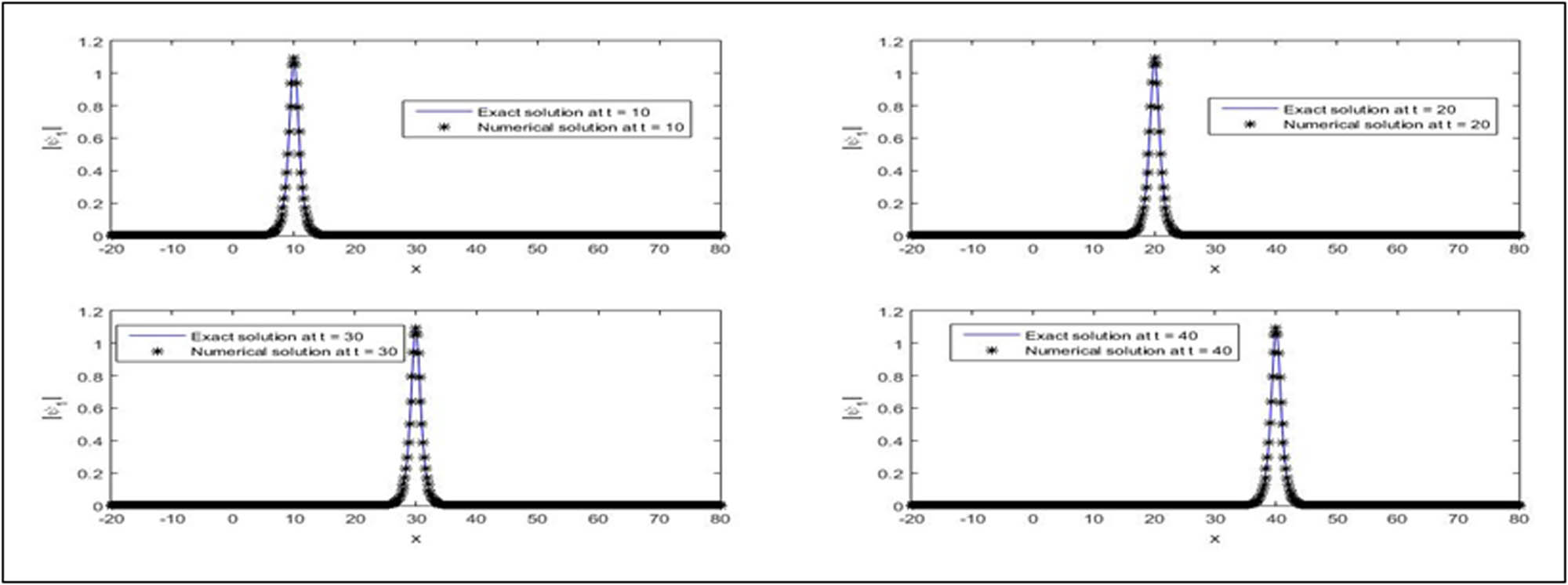
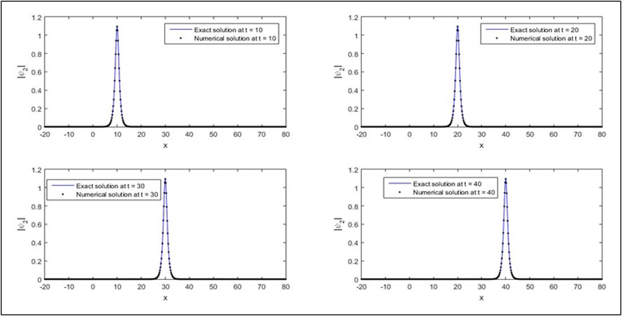
In present example, concept is related with the collision of two solitons, nature of wave propagation is verified, agreement of exact and numerical solutions is provided, and elasticity property of the interaction of two solitons is elaborated. In Figure 3, numerical and exact solutions for first-wave amplitude are matched at different time levels. At time levels, mentioned in figure, exact and numerical solutions are matched. In Figure 4, numerical and exact solutions are shown for second-wave amplitude at t = 1 , 2, 3, and 4. In Figure 5, two-soliton interaction is discussed. It is observed that on the changed time levels, solitons moved from left to right but shape of solitons could not remain same, because of this change in shape of solitons, it can be said that this interaction of two solitons for δ = 0.2 and e = 2 is inelastic. In Figure 6, the interaction of two solitons is presented for second-wave amplitude. As time level got changed, solitons moved from left to right, but the shapes of the solitons got fluctuated on changing time level. It means that the interaction of two solitons for δ = 0.2 and e = 2 is inelastic interaction. In Figure 7, the interaction of two solitons is shown for first-wave amplitude. In this interaction, higher-amplitude wave crossed lower-amplitude waves and moved from left to right on changing time level. The shapes of solitons were unchanged on changing time levels. It indicates that this interaction of two solitons is an elastic interaction for δ = 0.5 and e = 1 . In Figure 8, the interaction of two solitons is shown for second-wave amplitude. By changing time levels, higher amplitude wave crossed the lower ones, moved in right direction. In this interaction also shape of solitons remained unchanged with changed time levels. It means that this interaction of two solitons is an elastic interaction. In Table 5, L ∞ error norm is discussed for Ω 1 and Ω 2 at time levels 5, 10, 15, and 20. In Table 6, a comparison of the conserved quantities is given at different time levels with [17] for δ = 0.2 and δ = 0.5 , respectively. Present quantities are almost preserved.

$Figure 3 Numerical and exact values of first-wave amplitudes, respectively, for N = 501 N=501 , Δ t = 0.0001 \Delta t=0.0001 , β 1 = 1 {\beta }_{1}=1 , β 2 = 0.5 {\beta }_{2}=0.5 , ν 1 = 1 {\nu }_{1}=1 , ν 2 = 0.1 {\nu }_{2}=0.1 , e = 1 e=1 , and τ = 1 \tau =1 at t = 1 t=1 , 2, 3, and 4 [ − 20 , 80 -20,80 ].$

Figure 3

Numerical and exact values of first-wave amplitudes, respectively, for N = 501 , Δ t = 0.0001 , β 1 = 1 , β 2 = 0.5 , ν 1 = 1 , ν 2 = 0.1 , e = 1 , and τ = 1 at t = 1 , 2, 3, and 4 [ − 20 , 80 ].

$Figure 4 Numerical and exact values of second-wave amplitudes respectively for N = 201 N=201 , Δ t = 0.0001 \Delta t=0.0001 , β 1 = 1 {\beta }_{1}=1 , β 2 = 0.5 {\beta }_{2}=0.5 , ν 1 = 1 {\nu }_{1}=1 , ν 2 = 0.1 {\nu }_{2}=0.1 , e = 1 e=1 , τ = 1 \tau =1 at t = 1 t=1 , 2, 3, and 4 [ − 20 , 80 -20,80 ].$

Figure 4

Numerical and exact values of second-wave amplitudes respectively for N = 201 , Δ t = 0.0001 , β 1 = 1 , β 2 = 0.5 , ν 1 = 1 , ν 2 = 0.1 , e = 1 , τ = 1 at t = 1 , 2, 3, and 4 [ − 20 , 80 ].

$Figure 5 Interaction of two solitons for first-wave amplitude for N = 501 N=501 , Δ t = 0.01 \Delta t=0.01 , δ = 0.2 \delta =0.2 , β 1 = 1 {\beta }_{1}=1 , β 2 = 0.5 {\beta }_{2}=0.5 , ν 1 = 1 {\nu }_{1}=1 , ν 2 = 0.1 {\nu }_{2}=0.1 , e = 2 e=2 , τ = 1 \tau =1 [ − 20 , 80 -20,80 ].$

Figure 5

Interaction of two solitons for first-wave amplitude for N = 501 , Δ t = 0.01 , δ = 0.2 , β 1 = 1 , β 2 = 0.5 , ν 1 = 1 , ν 2 = 0.1 , e = 2 , τ = 1 [ − 20 , 80 ].

$Figure 6 Interaction of two solitons for second-wave amplitude for N = 501 N=501 , Δ t = 0.01 \Delta t=0.01 , δ = 0.2 \delta =0.2 , β 1 = 1 {\beta }_{1}=1 , β 2 = 0.5 {\beta }_{2}=0.5 , ν 1 = 1 {\nu }_{1}=1 , ν 2 = 0.1 {\nu }_{2}=0.1 , e = 2 e=2 , τ = 1 \tau =1 , [ − 20 , 80 -20,80 ].$

Figure 6

Interaction of two solitons for second-wave amplitude for N = 501 , Δ t = 0.01 , δ = 0.2 , β 1 = 1 , β 2 = 0.5 , ν 1 = 1 , ν 2 = 0.1 , e = 2 , τ = 1 , [ − 20 , 80 ].

$Figure 7 Interaction of two solitons for first-wave amplitude for N = 501 N=501 , Δ t = 0.01 \Delta t=0.01 , δ = 0.5 \delta =0.5 , β 1 = 1 {\beta }_{1}=1 , β 2 = 0.5 {\beta }_{2}=0.5 , ν 1 = 1 {\nu }_{1}=1 , ν 2 = 0.1 {\nu }_{2}=0.1 , and e = 1 e=1 [ − 20 , 80 -20,80 ].$

Figure 7

Interaction of two solitons for first-wave amplitude for N = 501 , Δ t = 0.01 , δ = 0.5 , β 1 = 1 , β 2 = 0.5 , ν 1 = 1 , ν 2 = 0.1 , and e = 1 [ − 20 , 80 ].

$Figure 8 Interaction of two solitons for second-wave amplitude for N = 501 N=501 , Δ t = 0.01 \Delta t=0.01 , δ = 0.5 \delta =0.5 , β 1 = 1 {\beta }_{1}=1 , β 2 = 0.5 {\beta }_{2}=0.5 , ν 1 = 1 {\nu }_{1}=1 , ν 2 = 0.1 {\nu }_{2}=0.1 , e = 1 e=1 , and τ = 1 \tau =1 [ − 20 , 80 -20,80 ].$

Figure 8

Interaction of two solitons for second-wave amplitude for N = 501 , Δ t = 0.01 , δ = 0.5 , β 1 = 1 , β 2 = 0.5 , ν 1 = 1 , ν 2 = 0.1 , e = 1 , and τ = 1 [ − 20 , 80 ].

Table 5

L ∞ error for two-soliton interaction for parameters N = 201 , β 1 = 1 , β 2 = 0.5 , ν 1 = 1 , ν 2 = 0.1 , e = 1 , and τ = 1 at different Δ t and different time levels, x l = − 20 and x r = 80

t	Δ t = 0.01		Δ t = 0.04		Δ t = 0.07
	L ∞ ψ 1	L ∞ ψ 2	L ∞ ψ 1	L ∞ ψ 2	L ∞ ψ 1	L ∞ ψ 2
5	1.67 × 1 0 − 6	1.70 × 1 0 − 6	1.05 × 1 0 − 4	1.05 × 1 0 − 4	5.38 × 1 0 − 4	5.39 × 1 0 − 4
10	− 2.94 × 1 0 − 4	2.48 × 1 0 − 4	− 3.61 × 1 0 − 5	4.76 × 1 0 − 4	1.01 × 1 0 − 3	1.41 × 1 0 − 3
15	− 6.16 × 1 0 − 4	4.87 × 1 0 − 4	− 1.62 × 1 0 − 4	8.61 × 1 0 − 4	1.61 × 1 0 − 3	2.37 × 1 0 − 3
20	− 2.80 × 1 0 − 3	− 1.04 × 1 0 − 3	− 2.10 × 1 0 − 3	− 4.91 × 1 0 − 4	4.94 × 1 0 − 4	1.62 × 1 0 − 3

Table 6

Comparison of conserved quantity for parameters N = 201 , Δ t = 0.01 , β 1 = 1 , β 2 = 0.5 , ν 1 = 1 , and ν 2 = 0.1 , τ = 1 for different δ and e , x l = − 20 and x r = 80

	δ = 0.2		δ = 0.5
Time level	I 1	I 1	I 1	I 1
	Ismail and Taha	[Present method]	Ismail and Taha	[Present method]
	[17]		[17]
10	1.70207	2.41455	1.70207	2.41493
20	1.70207	2.41518	1.70207	2.41631
30	1.70207	2.41568	1.70207	2.4176
40	1.70206	2.41621	1.70297	2.41995
50	1.70161	2.41702	1.70207	2.42843

Example 3

Collision of three solitons: In this example, 1D coupled CNLSE (1) and (2) are considered with the following initial conditions:

(56) Ω 1 ( x , 0 ) = ∑ j = 1 3 f j ( x ) ,

where

f j ( x ) = 2 β j ( 1 + e ) sech [ 2 β j ( x j ) ] exp i [ ( ν j − δ ) x j ] .

(57) Ω 2 ( x , 0 ) = ∑ k = 1 3 f k ( x )

and

f k ( x ) = 2 β k ( 1 + e ) sech [ 2 β k ( x k ) ] exp i [ ( ν k + δ ) x k ] .

In this example, interaction of three solitons is discussed. In Figure 9, interaction of three solitons is discussed for first-wave amplitude. It is observed that higher amplitude wave crossed lower amplitude waves on changing time levels and all solitons reserved their shapes because of this fact, this interaction of three solitons is an elastic interaction for δ = 0.5 and δ = 0.2. In Figure 10, interaction of three solitons is shown for second-wave amplitude. In this case also higher amplitude wave crossed the lower amplitude wave from left to right without any change in shapes of solitons. This interaction of three solitons for second-wave amplitude for δ = 0.5 is also an elastic interaction. In Figure 11, three soliton’s interaction is shown for first-wave amplitude, and higher-amplitude wave crossed the lower-amplitude waves and moved from left to right at the changed time levels but the shapes of solitons could not remain same. It indicates that this interaction is an inelastic interaction for δ = 0.2 and e = 2. In Figure 12, the interaction of three solitons is shown for the second-wave amplitude for δ = 0.2 and e = 2 . Higher-amplitude wave crossed the lower-amplitude waves but shapes got changed at different time levels. It means that given interaction is an inelastic interaction. In Table 7, comparison of the first conserved quantity is given with [17] for e = 2 3 and e = 1 . The present value of first conserved quantity is reserved up to three numerals.

$Figure 9 Interaction of three solitons for first-wave amplitude for Δ t = 0.001 \Delta t=0.001 , N = 501 N=501 , δ = 0.5 \delta =0.5 , e = 2 e=2 , β 1 = 1.2 {\beta }_{1}=1.2 , β 2 = 0.72 {\beta }_{2}=0.72 , β 3 = 0.36 {\beta }_{3}=0.36 , ν 1 = 1 {\nu }_{1}=1 , ν 2 = 0.1 {\nu }_{2}=0.1 , ν 3 = − 1 {\nu }_{3}=-1 , τ = 0.1 \tau =0.1 [ − 20 , 80 -20,80 ].$

Figure 9

Interaction of three solitons for first-wave amplitude for Δ t = 0.001 , N = 501 , δ = 0.5 , e = 2 , β 1 = 1.2 , β 2 = 0.72 , β 3 = 0.36 , ν 1 = 1 , ν 2 = 0.1 , ν 3 = − 1 , τ = 0.1 [ − 20 , 80 ].

$Figure 10 Interaction of three solitons for second-wave amplitude for Δ t = 0.001 \Delta t=0.001 , N = 501 N=501 , δ = 0.5 \delta =0.5 , e = 2 e=2 , β 1 = 1.2 {\beta }_{1}=1.2 , β 2 = 0.72 {\beta }_{2}=0.72 , β 3 = 0.36 {\beta }_{3}=0.36 , ν 1 = 1 {\nu }_{1}=1 , ν 2 = 0.1 {\nu }_{2}=0.1 , ν 3 = − 1 {\nu }_{3}=-1 , and τ = 0.1 \tau =0.1 [ − 20 , 80 -20,80 ].$

Figure 10

Interaction of three solitons for second-wave amplitude for Δ t = 0.001 , N = 501 , δ = 0.5 , e = 2 , β 1 = 1.2 , β 2 = 0.72 , β 3 = 0.36 , ν 1 = 1 , ν 2 = 0.1 , ν 3 = − 1 , and τ = 0.1 [ − 20 , 80 ].

$Figure 11 Interaction of three solitons for first-wave amplitude for Δ t = 0.001 \Delta t=0.001 , N = 501 N=501 , δ = 0.2 \delta =0.2 , e = 2 e=2 , β 1 = 1.2 {\beta }_{1}=1.2 , β 2 = 0.72 {\beta }_{2}=0.72 , β 3 = 0.36 {\beta }_{3}=0.36 , ν 1 = 1 {\nu }_{1}=1 , ν 2 = 0.1 {\nu }_{2}=0.1 , ν 3 = − 1 {\nu }_{3}=-1 , and τ = 0.1 \tau =0.1 [ − 20 , 80 -20,80 ].$

Figure 11

Interaction of three solitons for first-wave amplitude for Δ t = 0.001 , N = 501 , δ = 0.2 , e = 2 , β 1 = 1.2 , β 2 = 0.72 , β 3 = 0.36 , ν 1 = 1 , ν 2 = 0.1 , ν 3 = − 1 , and τ = 0.1 [ − 20 , 80 ].

$Figure 12 Interaction of three solitons for second-wave amplitude for Δ t = 0.001 \Delta t=0.001 , N = 501 N=501 , δ = 0.2 \delta =0.2 , e = 2 e=2 , β 1 = 1.2 {\beta }_{1}=1.2 , β 2 = 0.72 {\beta }_{2}=0.72 , β 3 = 0.36 {\beta }_{3}=0.36 , ν 1 = 1 {\nu }_{1}=1 , ν 2 = 0.1 {\nu }_{2}=0.1 , ν 3 = − 1 {\nu }_{3}=-1 , and τ = 0.1 \tau =0.1 [ − 20 , 80 -20,80 ].$

Figure 12

Interaction of three solitons for second-wave amplitude for Δ t = 0.001 , N = 501 , δ = 0.2 , e = 2 , β 1 = 1.2 , β 2 = 0.72 , β 3 = 0.36 , ν 1 = 1 , ν 2 = 0.1 , ν 3 = − 1 , and τ = 0.1 [ − 20 , 80 ].

Table 7

Comparison of conserved quantity for interaction of three solitons for Δ t = 0.01 , N = 301 , δ = 0.5 , β 1 = 1.2 , β 2 = 0.72 , β 3 = 0.36 , ν 1 = 1 , ν 2 = 0.1 , ν 3 = − 1 , and τ = 0.5 for different values of e at different time levels [ − 20 , 80 ]

Time level t	I 1 [17]	I 1 [Present]	I 1 [17]	I 1 [Present]
	e = 2 3			e = 1
10	2.0778	4.31725	1.89677	3.59771
20	2.0778	4.31724	1.89677	3.5977
30	2.0778	4.31718	1.89677	3.59765
40	2.0778	4.31748	1.89677	3.59787
50	2.0778	4.31755	1.89668	3.59791

Example 4

In this example, 2D CNLSE (7) and (8) with following I.C.s [14] are as follows:

(58) Ω 1 ( x , y , 0 ) = λ sech ( β 1 x + β 2 y ) exp [ i − k 1 x − k 2 y ] ,

(59) Ω 2 ( x , y , 0 ) = λ sech ( β 1 x + β 2 y ) exp [ i − k 1 x − k 2 y ] ,

where λ = β 1 2 + β 2 2 1 + α .

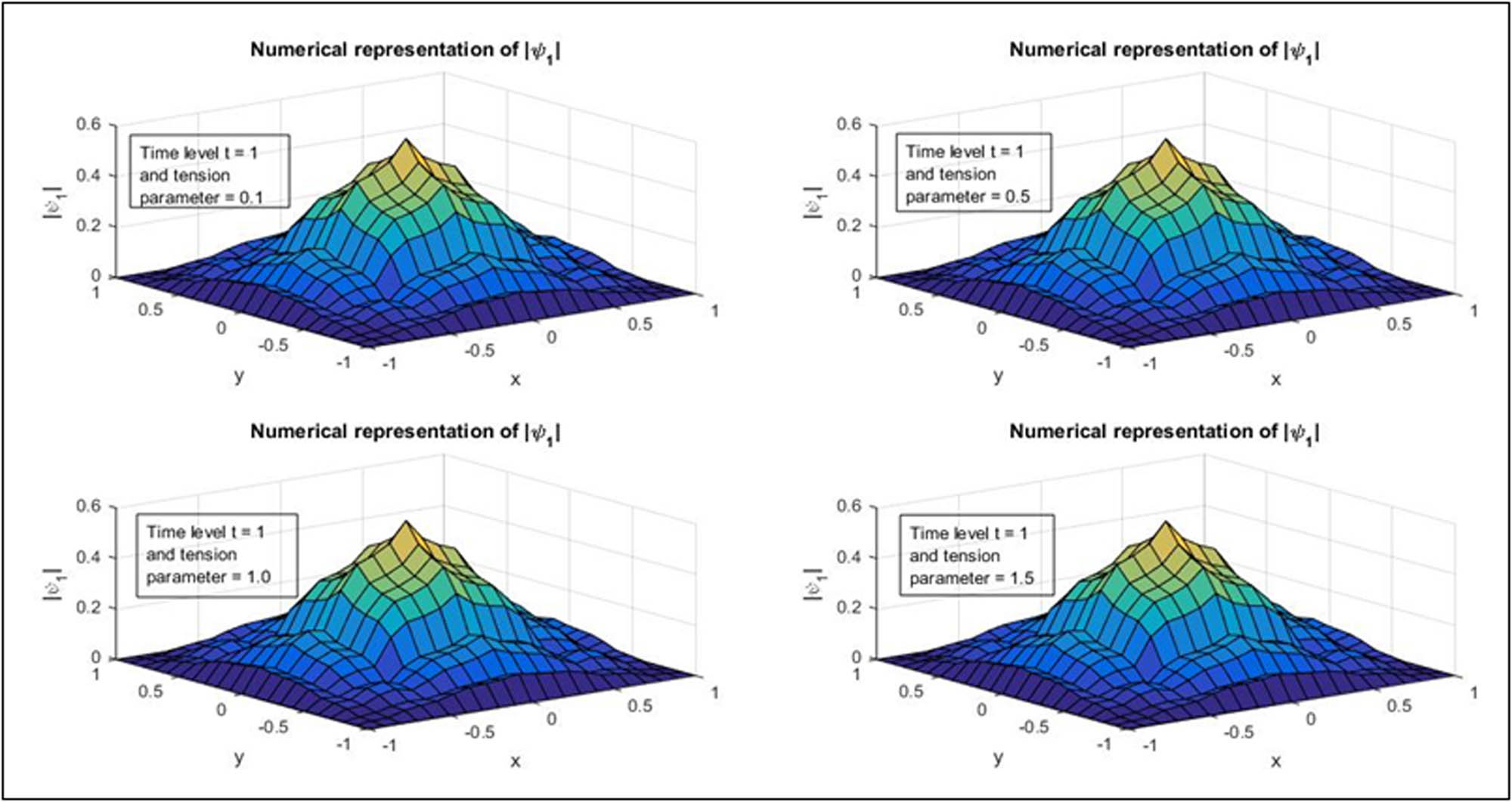
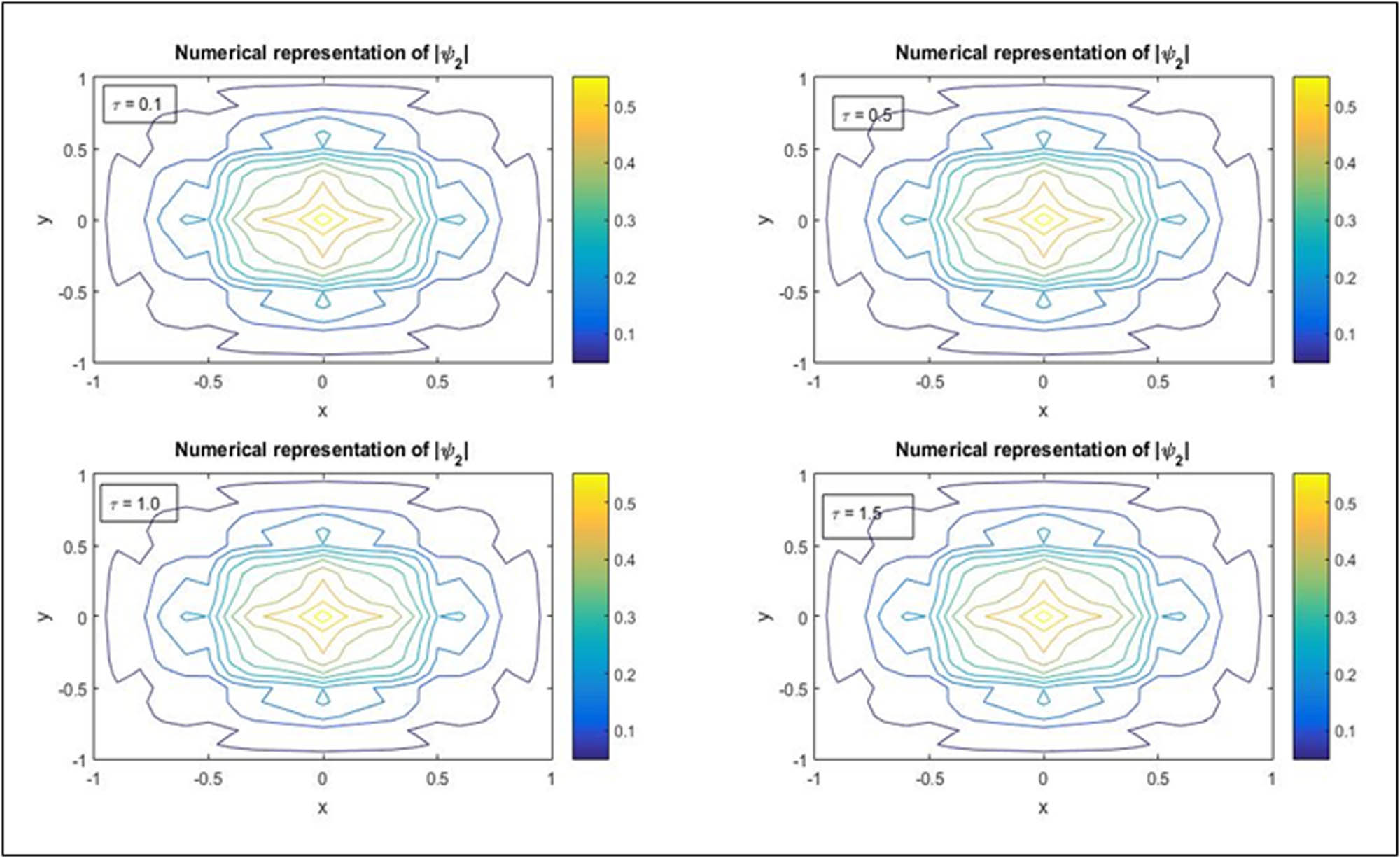
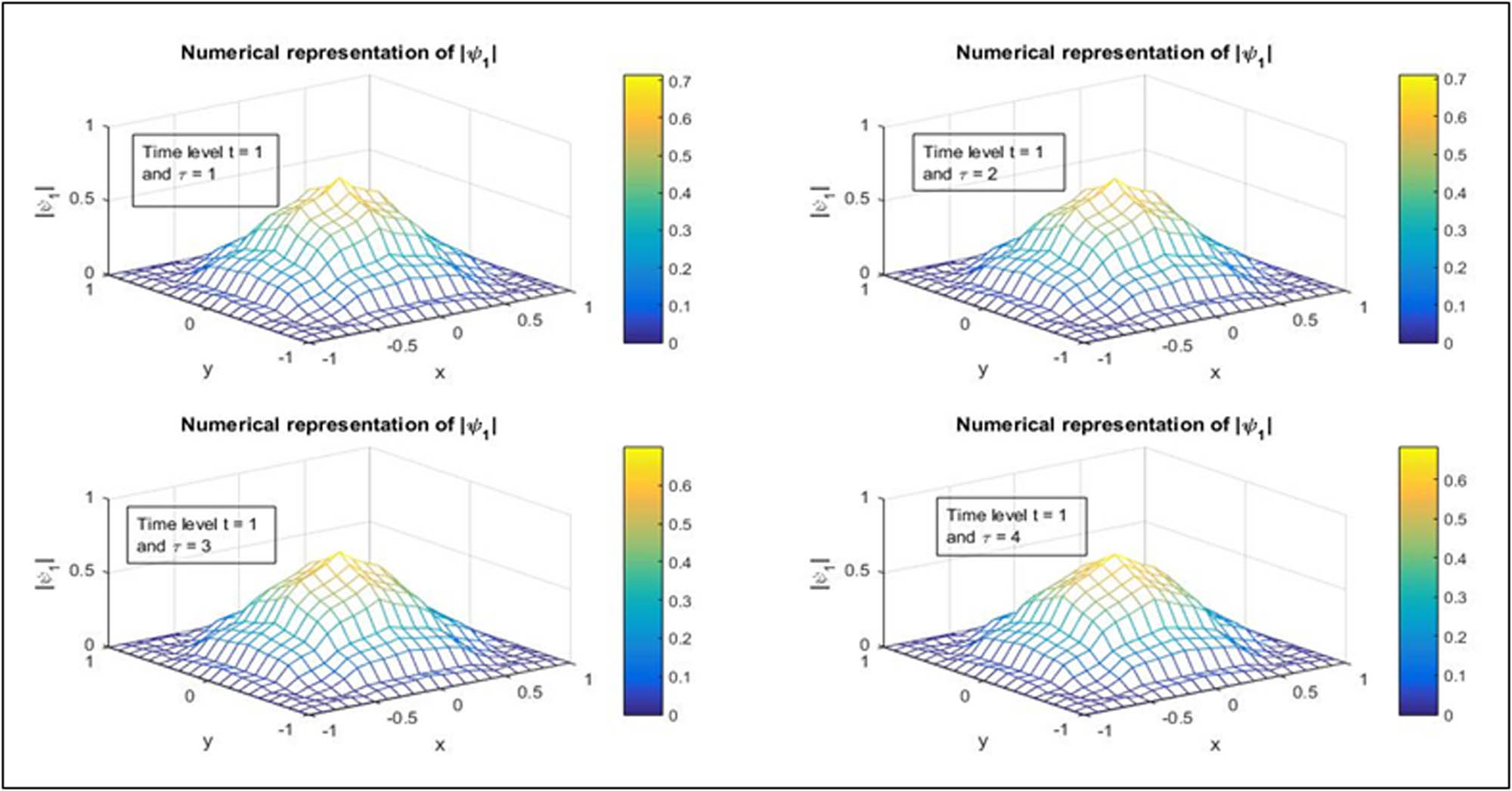
In this example, exact solution of problem is not provided, only I.C.s are given with computational domain. In such case, we have discussed numerical solution for first- and second-wave amplitudes. In Figure 13, numerical solution of the first-wave amplitude is represented at t = 1 , 2, 3 and 4, respectively. In Figure 14, the numerical solution of the second-wave amplitude is shown at t = 1 , 2, 3, and 4.

$Figure 13 Representation of numerical solution of first-wave amplitude with N = 51 N=51 , Δ t = 0.001 \Delta t=0.001 , β 1 = 0.5 {\beta }_{1}=0.5 , β 2 = 1 {\beta }_{2}=1 , k 1 = 1.0 {k}_{1}=1.0 , k 2 = 1.0 {k}_{2}=1.0 , and α = 1 \alpha =1 at t = 1 t=1 , 2, 3, and 4, τ = 1 \tau =1 [ − 10 , 10 -10,10 ].$

Figure 13

Representation of numerical solution of first-wave amplitude with N = 51 , Δ t = 0.001 , β 1 = 0.5 , β 2 = 1 , k 1 = 1.0 , k 2 = 1.0 , and α = 1 at t = 1 , 2, 3, and 4, τ = 1 [ − 10 , 10 ].

$Figure 14 Representation of numerical solution of second-wave amplitude with N = 51 N=51 , Δ t = 0.001 \Delta t=0.001 , β 1 = 0.5 {\beta }_{1}=0.5 , β 2 = 1 {\beta }_{2}=1 , k 1 = 1.0 {k}_{1}=1.0 , k 2 = 1.0 {k}_{2}=1.0 , and α = 1 \alpha =1 at t = 1 t=1 , 2, 3, and 4, τ = 1 \tau =1 [ − 10 , 10 -10,10 ].$

Figure 14

Representation of numerical solution of second-wave amplitude with N = 51 , Δ t = 0.001 , β 1 = 0.5 , β 2 = 1 , k 1 = 1.0 , k 2 = 1.0 , and α = 1 at t = 1 , 2, 3, and 4, τ = 1 [ − 10 , 10 ].

Example 5

In this example, 2D CNLSEs (7) and (8) are considered with the following initial conditions [18]:

(60) Ω 1 ( x , y , 0 ) = 2 α 1 + π sech [ ( x − x 1 , l ) ( y − y 2 , l ) ( x − x 1 , r ) ( y − y 1 , R ) ] ,

(61) Ω 2 ( x , y , 0 ) = 2 α 1 + π sech [ ( x − x 1 , l ) ( y − y 2 , l ) ( x − x 1 , r ) ( y − y 1 , R ) ] ,

where boundary conditions are,

∂ Ω 1 ∂ x = 0 , t ≥ 0 , ∂ Ω 2 ∂ x = 0 , t ≥ 0 ,

where consideration is x 1 , l = x 2 , l = − 1 and y 1 , l = y 2 , l = − 1 .

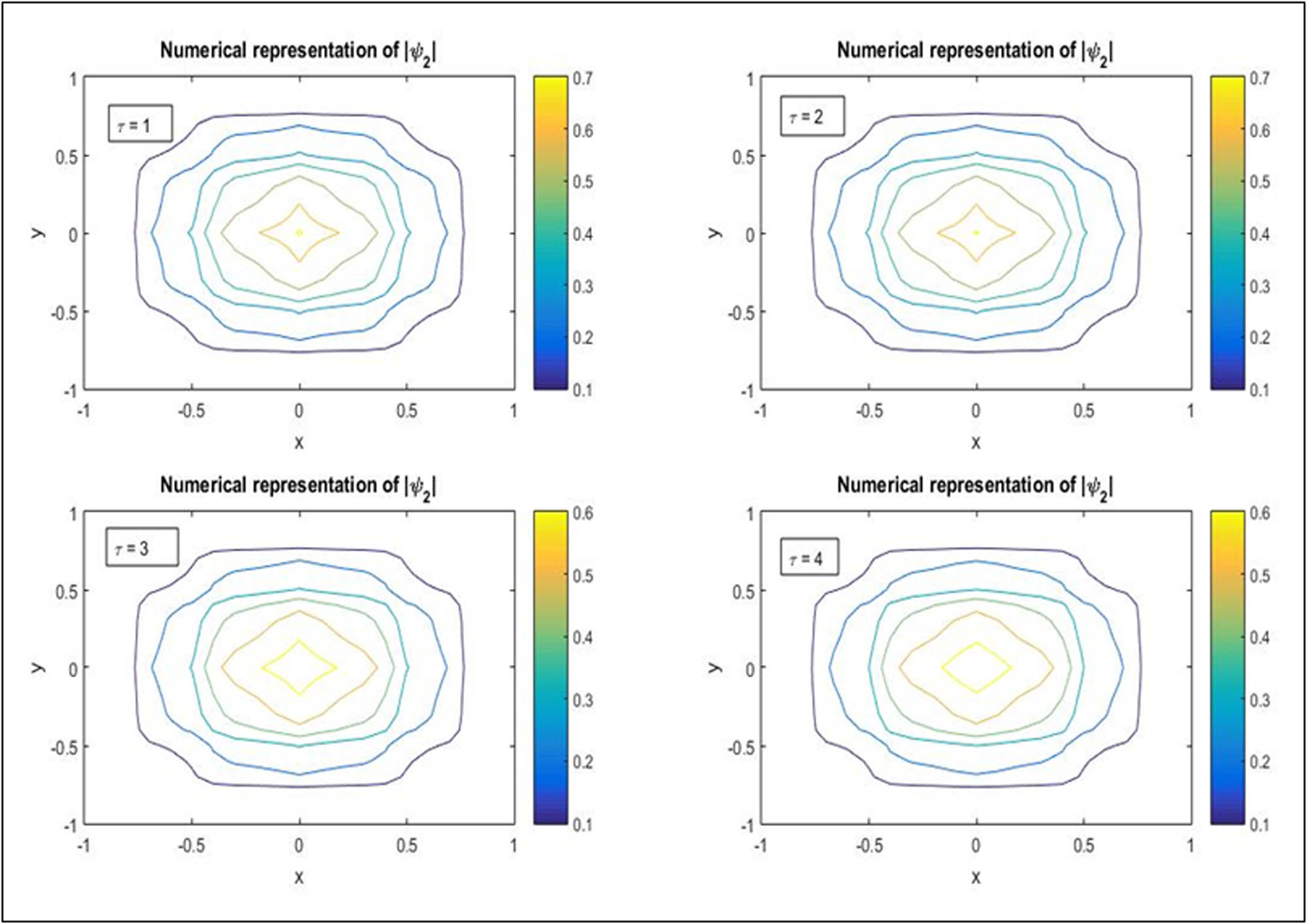
In this example, only numerical solution is discussed, as analytical solution of the present problem is not given. In Figure 15, the graphical representation of numerical solution of first-wave amplitude is shown at t = 1 and for different values of tension parameters. In Figure 16, contour representation of numerical solution of second-wave amplitude is shown at t = 1 and for different values of tension parameters.

$Figure 15 Graphical representation of numerical solution of first-wave amplitude at t = 1 t=1 for parameters, N = 21 N=21 , Δ t = 0.0001 \Delta t=0.0001 , α = 0.1 \alpha =0.1 and for different values of tension parameter τ \tau .$

Figure 15

Graphical representation of numerical solution of first-wave amplitude at t = 1 for parameters, N = 21 , Δ t = 0.0001 , α = 0.1 and for different values of tension parameter τ .

$Figure 16 Graphical representation of numerical solution of second-wave amplitude at t = 1 t=1 for parameters, N = 21 N=21 , Δ t = 0.0001 \Delta t=0.0001 , and α = 0.1 \alpha =0.1 and for different values of tension parameter τ \tau .$

Figure 16

Graphical representation of numerical solution of second-wave amplitude at t = 1 for parameters, N = 21 , Δ t = 0.0001 , and α = 0.1 and for different values of tension parameter τ .

Example 6

In this example, 2D CNLSEs (7) and (8) are considered with the following initial conditions [18]:

(62) Ω 1 ( x , y , 0 ) = 2 α 1 + π cosh [ ( x − x 1 , l ) ( y − y 2 , l ) ( x − x 1 , r ) ( y − y 1 , R ) ] ,

(63) Ω 2 ( x , y , 0 ) = 2 α 1 + π cosh [ ( x − x 1 , l ) ( y − y 2 , l ) ( x − x 1 , r ) ( y − y 1 , R ) ] ,

where boundary conditions are,

∂ Ω 1 ∂ t = 0 , t ≥ 0 , ∂ Ω 2 ∂ t = 0 , t ≥ 0 ,

where consideration is x 1 , l = x 2 , l = − 1 and y 1 , l = y 2 , l = − 1 .

In Figure 17, the numerical solution of first-wave amplitude is shown at t = 1 and for different values of tension parameter. In Figure 18, contour representation of numerical solution of second-wave amplitude is given at t = 1 and for different values of tension parameters.

$Figure 17 Graphical representation of numerical solution of first-wave amplitude at t = 1 t=1 for parameters N = 21 N=21 , Δ t = 0.0001 \Delta t=0.0001 , and α = 0.1 \alpha =0.1 and for different values of tension parameter τ \tau .$

Figure 17

Graphical representation of numerical solution of first-wave amplitude at t = 1 for parameters N = 21 , Δ t = 0.0001 , and α = 0.1 and for different values of tension parameter τ .

$Figure 18 Graphical representation of numerical solution of second-wave amplitude at t = 1 t=1 for parameters N = 21 N=21 , Δ t = 0.0001 \Delta t=0.0001 , α = 0.1 \alpha =0.1 and for different values of tension parameter τ \tau .$

Figure 18

Graphical representation of numerical solution of second-wave amplitude at t = 1 for parameters N = 21 , Δ t = 0.0001 , α = 0.1 and for different values of tension parameter τ .

The main outcomes from graphical and tabular discussion. In the present study, a detailed study is done via Graphs and Tables. Some of the noteworthy points of the mentioned discussion are notified as follows:

Via Figures 1 and 2, the compatibility property of the approx. and exact results is claimed for single soliton.
Via Figures 3 and 4, the compatibility property of the approx. and exact results is notified for two solitons.
Via Figures 5–8, the elasticity property of two-soliton interaction is claimed.
Via Figure 9–12, the elasticity property of three soliton interaction is notified.
Via Figure 13–18, the numerical solutions are provided where exact solutions are not available in the literature.
Via Table 2, the obtained results of L ∞ error are much better than the compared one.
Via Table 3, the conservation property of the conserved quantities is claimed.

4 Stability

By implementing discretization formulae of partial derivatives in Eqs. (1) and (2), the following system of equations will be obtained:

(64) d ϕ d t = − δ ∑ j = 1 N q i j ( 1 ) ϕ ( x j ) + i 2 ∑ j = 1 N q i j ( 2 ) ϕ ( x j ) + i [ ∣ ϕ ∣ 2 + e ∣ θ ∣ 2 ] ϕ ,

(65) d θ d t = δ ∑ j = 1 N q i j ( 1 ) θ ( x j ) + i 2 ∑ j = 1 N q i j ( 2 ) θ ( x j ) + i [ e ∣ ϕ ∣ 2 + ∣ θ ∣ 2 ] θ .

The above system of equations can be written as follows:

(66) d ϕ d t d θ d t = T 1 ϕ θ + h [ ϕ ( x , t ) ] ,

where matrix is obtained using ODE system and h [ ϕ ( x , t ) ] is the corresponding nonlinear term. The stability of the ODE system depends upon eigen values of matrix T 1 , which is given as follows:

T 1 = M 1 O O M 2 ,

where

M 1 = − δ q i j ( 1 ) + i 2 q i j ( 2 ) Δ t , M 2 = δ q i j ( 1 ) + i 2 q i j ( 2 ) Δ t .

Via discretization formula in Eqs. (7) and (8), a novel ODE system will be obtained:

(67) d ϕ d t = i 2 ∑ j = 1 N 1 η i j ϕ ( x j , y , t ) + ∑ j = 1 N 2 η i j ′ ϕ ( x , y j , t ) + i [ ∣ ϕ ∣ 2 + α ∣ θ ∣ 2 ] ϕ ,

(68) d θ d t = i 2 ∑ j = 1 N 1 η i j θ ( x j , y , t ) + ∑ j = 1 N 2 η i j ′ θ ( x , y j , t ) + i [ α ∣ ϕ ∣ 2 + ∣ θ ∣ 2 ] θ .

ODE system can be written as follows:

(69) d ϕ d t d θ d t = T 2 ϕ θ + h [ ϕ ( x , y , t ) ] .

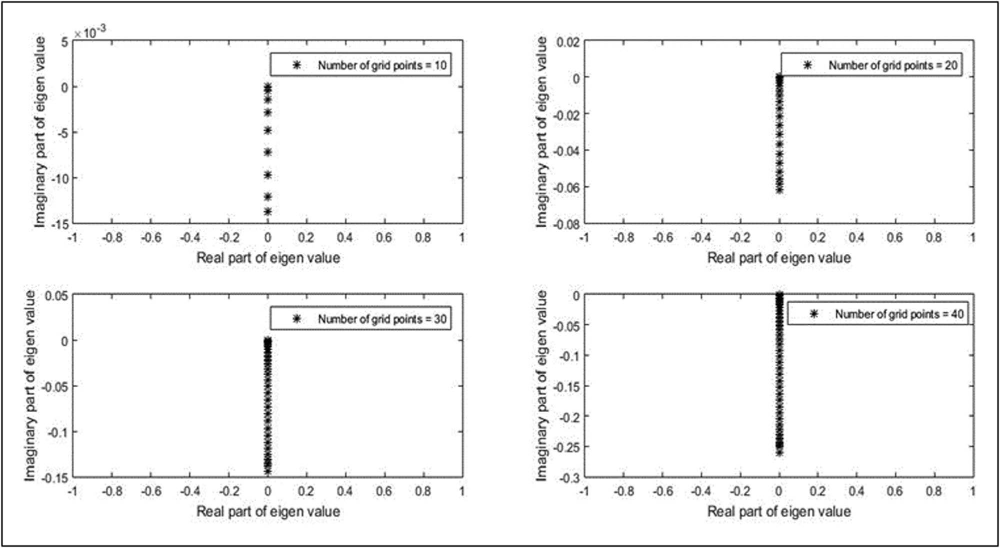
The stability of the present scheme will depend upon eigen values of matrix T 2 , and h [ ϕ ( x , y , t ) ] is the corresponding nonlinear term.

T 2 = N 1 O O N 2 ,

where

N 1 = i 2 { η i j + η i j ′ } Δ t , N 2 = i 2 { η i j + η i j ′ } Δ t .

Obtained ODE system will be stable if eigen values of matrices B 1 and B 2 are in the following range:

Real λ : − 2.78 < Δ t < 0 .
Pure Imaginary λ : − 2 2 < λ Δ t < 2 2 .
Complex λ : λ Δ t will be in the region presented in Figure 19. The stability of the proposed method here is discussed via the matrix method and the graphical representation is provided in Figures 20 and 21, respectively. These figures indicates that obtained eigen values are within the prescribed range. It can be said that present scheme is unconditionally stable.

Figure 19

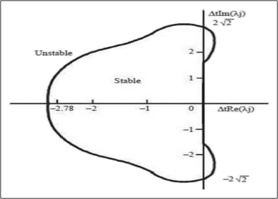
Stability criteria.

Figure 20

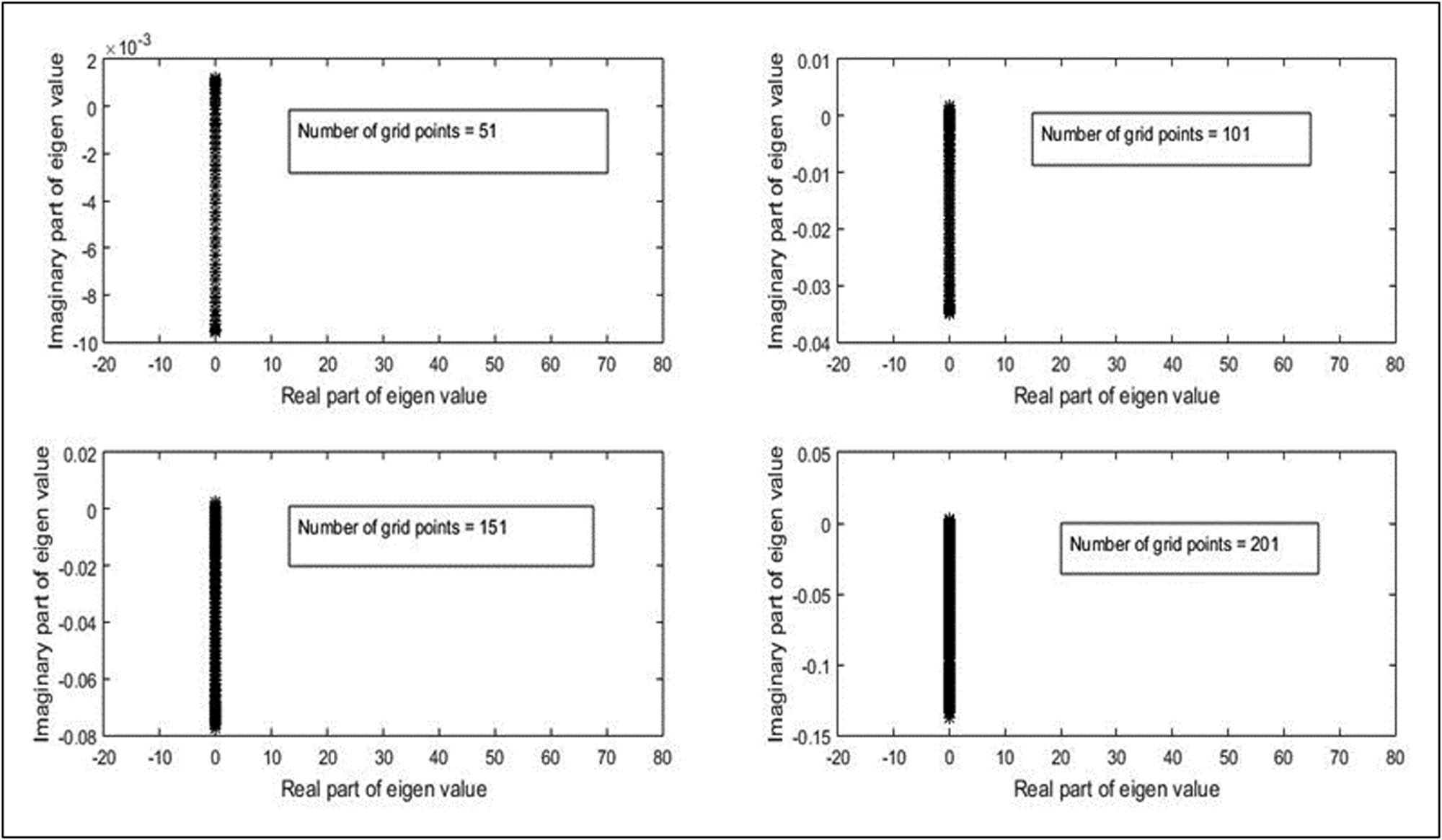
The stability of the present method in one dimension at different number of grid points.

Figure 21

The stability of the present method in two dimension at different number of grid points.

5 Conclusion

In this article, a novel scheme, UAH tension B-spline-based DQM is implemented upon coupled 1D and -2D Schrödinger equations, respectively. Spatial discretization is done with the aid of UAH tension B-spline of fourth-order. In Section 2.4, the process of finding is discussed. The reduced set of ODEs is tackled with the SSP-RK43 scheme. In the present study, six examples are discussed to affirm the validity of developed regime. By comparing present results with the existing results in literature, it can be affirmed that developed scheme is acceptable. Elastic property for solitons is also discussed. The stability of the proposed regime is discussed with matrix method in Section 4. By observing fetched results of this present work, it can be claimed that this research work will be helpful for different researchers in their future research work so that some new dimensions in this area can be explored.

The main advantage of this article is to deal with the numerical approximation of the coupled nonlinear Schrödinger equation. Finding the numerical solution to such complex-natured equations is not an easy task. Therefore, as a research gap, a novel technique is developed with a fusion of UAH tension B-spline and DQM. In this manuscript, the main motive is to provide improvised and more sustainable numerical results. Via Figures 1 and 2, the compatibility property of the approx. and exact results is claimed for single soliton. Via Figures 3 and 4, the compatibility property of the approx. and exact results is notified for two solitons. Via Figures 5–8, the elasticity property of two-soliton interaction is claimed. Via Figures 9–12, elasticity property of three-soliton interaction is notified. With the aid of Table 2, it is ensured that the obtained L ∞ errors are much reduced than compared results.

The future scope of the developed numerical regime is to deal with the complex nature ODEs, PDEs, integro, partial-integro, and fractional differential equations. As finding an exact solution of such cumbersome equations is not an easy task, the developed regime will be surely helpful for readers to deal with other equations of importance.

Funding information: Not available.
Author contributions: All authors have accepted responsibility for the entire content of this manuscript and approved its submission.
Conflict of interest: The authors have no conflict of interest.
Data availability statement: All data are included inside the manuscript.

References

[1] Korkmaz A, Dağ Í. A differential quadrature algorithm for nonlinear Schrödinger equation. Nonlinear Dyn. 2009;56(1–2):69–83. 10.1007/s11071-008-9380-0Search in Google Scholar

[2] Başhan A, Uçar Y, Yağmurlu NM, Esen A. A new perspective for quintic B-spline based Crank-Nicolson-differential quadrature method algorithm for numerical solutions of the nonlinear Schrödinger equation. Europ Phys J Plus. 2018;133(1):1–15. 10.1140/epjp/i2018-11843-1Search in Google Scholar

[3] Aksoy A, Irk D, Dag I. Taylor collocation method for the numerical solution of the nonlinear Schrödinger equation using quintic B-spline basis. Phys Wave Phenomena. 2012;20(1):67–79. 10.3103/S1541308X12010086Search in Google Scholar

[4] Robinson M. The solution of nonlinear Schrödinger equations using orthogonal spline collocation. Comput Math Appl. 1997;33(7):39–57. 10.1016/S0898-1221(97)00042-4Search in Google Scholar

[5] Gardner L, Gardner G, Zaki S, ElSahrawi Z. B-spline finite element studies of the non-linear Schrödinger equation. Comput Meth Appl Mech Eng. 1993;108(3–4):303–18. 10.1016/0045-7825(93)90007-KSearch in Google Scholar

[6] Bashan A, Yagmurlu NM, Ucar Y, Esen A. An effective approach to numerical soliton solutions for the Schrödinger equation via modified cubic B-spline differential quadrature method. Chaos Solitons Fractals. 2017;100:45–56. 10.1016/j.chaos.2017.04.038Search in Google Scholar

[7] Arora G, Joshi V, Mittal R. Numerical simulation of nonlinear Schrödinger equation in one and two dimensions. Math Models Comput Simulat. 2019;11(4):634–48. 10.1134/S2070048219040070Search in Google Scholar

[8] Wang H. Numerical studies on the split-step finite difference method for nonlinear Schrödinger equations. Appl Math Comput. 2005;170(1):17–35. 10.1016/j.amc.2004.10.066Search in Google Scholar

[9] Ismail M, Taha TR. A linearly implicit conservative scheme for the coupled nonlinear Schrödinger equation. Math Comput Simulat. 2007;74(4–5):302–11. 10.1016/j.matcom.2006.10.020Search in Google Scholar

[10] Ismail M. Numerical solution of coupled nonlinear Schrödinger equation by Galerkin method. Math Comput Simulat. 2008;78(4):532–47. 10.1016/j.matcom.2007.07.003Search in Google Scholar

[11] Sonnier W, Christov C. Strong coupling of Schrödinger equations: Conservative scheme approach. Math Comput Simulat. 2005;69(5–6):514–25. 10.1016/j.matcom.2005.03.016Search in Google Scholar

[12] Ismail M. A fourth-order explicit schemes for the coupled nonlinear Schrödinger equation. Appl Math Comput. 2008;196(1):273–84. 10.1016/j.amc.2007.05.059Search in Google Scholar

[13] Sweilam NH, Al-Bar R. Variational iteration method for coupled nonlinear Schrödinger equations. Comput Math Appl. 2007;54(7–8):993–9. 10.1016/j.camwa.2006.12.068Search in Google Scholar

[14] Ismail M, Ashi H, Al-Rakhemy F. ADI method for solving the two-dimensional coupled nonlinear Schrödinger equation. AIP Conf Proc. 2015;1648:050008.10.1063/1.4912368Search in Google Scholar

[15] Sun JQ, Qin MZ. Multi-symplectic methods for the coupled 1D nonlinear Schrödinger system. Comput Phys Commun. 2003;155(3):221–35. 10.1016/S0010-4655(03)00285-6Search in Google Scholar

[16] Abazari R, Abazari R. Numerical study of some coupled PDEs by using differential transformation method. Int J Math Comput Sci. 2010;4(6):641–8. Search in Google Scholar

[17] Ismail M, Taha TR. Numerical simulation of coupled nonlinear Schrödinger equation. Math Comput Simulat. 2001;56(6):547–62. 10.1016/S0378-4754(01)00324-XSearch in Google Scholar

[18] Dehghan M, Abbaszadeh M, Mohebbi A. Numerical solution of system of n-coupled nonlinear Schrödinger equations via two variants of the meshless local Petrov-Galerkin (MLPG) method. Comput Model Eng Sci. 2014;100(5):399–444. Search in Google Scholar

[19] Wadati M, Iizuka T, Hisakado M. A coupled nonlinear Schrödinger equation and optical solitons. J Phys Soc Japan. 1992;61(7):2241–5. 10.1143/JPSJ.61.2241Search in Google Scholar

[20] Bellman R, Kashef B, Casti J. Differential quadrature: a technique for the rapid solution of nonlinear partial differential equations. J Comput Phys. 1972;10(1):40–52. 10.1016/0021-9991(72)90089-7Search in Google Scholar

[21] Quan J, Chang C. New insights in solving distributed system equations by the quadrature method-I. Anal Comput Chem Eng. 1989;13(7):779–88. 10.1016/0098-1354(89)85051-3Search in Google Scholar

[22] Quan J, Chang CT. New insights in solving distributed system equations by the quadrature method-II. Numer Experiments Comput Chem Eng. 1989;13(9):1017–24. 10.1016/0098-1354(89)87043-7Search in Google Scholar

[23] Shu C. Generalized differential-integral quadrature and application to the simulation of incompressible viscous flows including parallel computation [dissertation]. Glasgow: University of Glasgow; 1991.Search in Google Scholar

[24] Korkmaz A, Dağ I. Shock wave simulations using Sinc differential quadrature method. Eng Comput. 2011;28(6):654–74.10.1108/02644401111154619Search in Google Scholar

[25] Mittal R, Bhatia R. A numerical study of two dimensional hyperbolic telegraph equation by modified B-spline differential quadrature method. Appl Math Comput. 2014;244:976–97. 10.1016/j.amc.2014.07.060Search in Google Scholar

[26] Shukla H, Tamsir M, Jiwari R, Srivastava VK. A numerical algorithm for computation modelling of 3D nonlinear wave equations based on exponential modified cubic B-spline differential quadrature method. Int J Comput Math. 2018;95(4):752–66. 10.1080/00207160.2017.1296573Search in Google Scholar

[27] Mittal RC, Dahiya S. A comparative study of modified cubic B-spline differential quadrature methods for a class of nonlinear viscous wave equations. Eng Comput. 2018;35(1):315–33.10.1108/EC-06-2016-0188Search in Google Scholar

[28] Zhang J. C-curves: an extension of cubic curves. Comput. Aided Geometric Design. 1996;13(3):199–217. 10.1016/0167-8396(95)00022-4Search in Google Scholar

[29] Zhang J. Two different forms of CB-splines. Comput Aided Geometric Design. 1997;14(1):31–41. 10.1016/S0167-8396(96)00019-2Search in Google Scholar

[30] Koch PE, Lyche T. Construction of exponential tension B-splines of arbitrary order. Curves Surf. 1991:255–8.10.1016/B978-0-12-438660-0.50039-XSearch in Google Scholar

[31] Lü Y, Wang G, Yang X. Uniform hyperbolic polynomial B-spline curves. Comput Aided Geometric Design. 2002;19(6):379–93. 10.1016/S0167-8396(02)00092-4Search in Google Scholar

[32] Wang G, Chen Q, Zhou M. NUAT B-spline curves. Comput Aided Geometric Design. 2004;21(2):193–205. 10.1016/j.cagd.2003.10.002Search in Google Scholar

[33] Jena MK, Shunmugaraj P, Das P. A subdivision algorithm for trigonometric spline curves. Comput Aided Geometric Design. 2002;19(1):71–88. 10.1016/S0167-8396(01)00090-5Search in Google Scholar

[34] Jena MK, Shunmugaraj P, Das P. A non-stationary subdivision scheme for generalizing trigonometric spline surfaces to arbitrary meshes. Comput Aided Geometric Design. 2003;20(2):61–77. 10.1016/S0167-8396(03)00008-6Search in Google Scholar

[35] Ya-Juan L, Guo-Zhao W. Two kinds of B-basis of the algebraic hyperbolic space. J Zhejiang Univ-Sci A. 2005;6(7):750–9. 10.1631/jzus.2005.A0750Search in Google Scholar

[36] Xu G, Wang GZ. AHT Bézier curves and NUAHT B-spline curves. J Comput Sci Technol. 2007;22(4):597–607. 10.1007/s11390-007-9073-zSearch in Google Scholar

[37] Alinia N, Zarebnia M. A new tension B-spline method for third-order self-adjoint singularly perturbed boundary value problems. J Comput Appl Math. 2018;342:521–33. 10.1016/j.cam.2018.03.021Search in Google Scholar

[38] Alinia N, Zarebnia M. A numerical algorithm based on a new kind of tension B-spline function for solving Burgers-Huxley equation. Numer Algor. 2019;82(4):1121–42. 10.1007/s11075-018-0646-4Search in Google Scholar

[39] ErsoyHepson O, Yigit G. Quartic-trigonometric tension B-spline Galerkin method for the solution of the advection-diffusion equation. Comput Appl Math. 2021;40(4):1–15. 10.1007/s40314-021-01526-2Search in Google Scholar

[40] ErsoyHepson O. Numerical simulations of Kuramoto-Sivashinsky equation in reaction-diffusion via Galerkin method. Math Sci. 2021;15(2):199–206. 10.1007/s40096-021-00402-8Search in Google Scholar

[41] Hepson OE, Dag I. Numerical investigation of the solutions of Schrödinger equation with exponential cubic B-spline finite element method. Int J Nonlinear Sci Numer Simulat. 2021;22(2):119–33. 10.1515/ijnsns-2016-0179Search in Google Scholar

[42] Nourian F, Lakestani M, Sabermahani S, Ordokhani Y. Touchard wavelet technique for solving time-fractional Black-Scholes model. Comput Appl Math. 2022;41(4):1–19. 10.1007/s40314-022-01853-ySearch in Google Scholar

[43] Başhan A. A mixed methods approach to Schrödinger equation: Finite difference method and quartic B-spline based differential quadrature method. Int J Optim Control Theories Appl (IJOCTA). 2019;9(2):223–35. 10.11121/ijocta.01.2019.00709Search in Google Scholar

[44] Başhan A, Uçar Y, Yağmurlu NM, Esen A. Numerical approximation to the MEW equation for the single solitary wave and different types of interactions of the solitary waves. J Differ Equ Appl. 2022;28(9):1–21. 10.1080/10236198.2022.2132154Search in Google Scholar

[45] Başhan A. Nonlinear dynamics of the Burgers’ equation and numerical experiments. Math Sci. 2022;16(2):183–205. 10.1007/s40096-021-00410-8Search in Google Scholar

[46] Başhan A. A numerical treatment of the coupled viscous Burgers’ equation in the presence of very large Reynolds number. Phys A Stat Mech Appl. 2020;545:123755. 10.1016/j.physa.2019.123755Search in Google Scholar

[47] Başhan A. Highly efficient approach to numerical solutions of two different forms of the modified Kawahara equation via contribution of two effective methods. Math Comput Simulat. 2021;179:111–25. 10.1016/j.matcom.2020.08.005Search in Google Scholar

[48] Başhan A, Yağmurlu NM. A mixed method approach to the solitary wave, undular bore and boundary-forced solutions of the Regularized Long Wave equation. Comput Appl Math. 2022;41(4):1–20. 10.1007/s40314-022-01882-7Search in Google Scholar

[49] Singh J, Alshehri AM, Momani S, Hadid S, Kumar D. Computational analysis of fractional diffusion equations occurring in oil pollution. Mathematics. 2022;10(20):3827. 10.3390/math10203827Search in Google Scholar

[50] Singh J, Kumar D, Purohit SD, Mishra AM, Bohra M. An efficient numerical approach for fractional multidimensional diffusion equations with exponential memory. Numer Meth Partial Differ Equ. 2021;37(2):1631–51. 10.1002/num.22601Search in Google Scholar

[51] Arora G, Singh BK. Numerical solution of Burgers’ equation with modified cubic B-spline differential quadrature method. Appl Math Comput. 2013;224:166–77. 10.1016/j.amc.2013.08.071Search in Google Scholar

Received: 2022-10-11

Revised: 2023-01-11

Accepted: 2023-02-12

Published Online: 2023-03-24

This work is licensed under the Creative Commons Attribution 4.0 International License.

Articles in the same Issue

https://doi.org/10.1515/nleng-2022-0283

Keywords for this article

DQM; UAH tension B-spline; coupled Schrödinger equations; SSP-RK 43 regime; matrix method

Creative Commons

BY 4.0