On duality principles and related convex dual formulations suitable for local and global non-convex variational optimization

Abstract
This article develops duality principles, a related convex dual formulation and primal dual formulations suitable for the local and global optimization of non convex primal formulations for a large class of models in physics and engineering. The results are based on standard tools of functional analysis, calculus of variations and duality theory. In particular, we develop applications to a Ginzburg–Landau type equation. Other applications include primal dual variational formulations for a Burger’s type equation and a Navier–Stokes system. We emphasize the novelty here is that the first dual variational formulation developed is convex for a primal formulation which is originally non-convex. Finally, we also highlight the primal dual variational formulations presented have a large region of convexity around any of their critical points.
1 Introduction
In the first part of this article, we establish a duality principle and a related convex dual formulation suitable for the local optimization of a primal formulation for a large class of models in non-convex optimization. We highlight that the first dual variational formulation presented is convex, and such a feature may be very useful for a large class of similar models, in particularly for large systems in a three or higher dimensional context.
For such a large system, the convexity obtained is relevant for an easier numerical computation, since in such a case of strict convexity, the standard Newton, Newton-type, and other similar methods are always convergent.
We also emphasize that the main duality principle is applied to the Ginzburg–Landau system in superconductivity in the absence of a magnetic field.
Other applications include primal dual formulations for a Burger’s type equation and a Navier–Stokes system.
For the duality principles, the results are based on the works of Telega and Bielski [1–4] and on a DC optimization approach developed in the study by Toland [5].
About the other references, details on the Sobolev spaces involved are found in the study by Adams and Fournier [6]. Related and more recent results on convex analysis and duality theory are addressed in the previous studies [7–11]. In particular, the results in the present work are extensions, and improvements of those results found in the recent book [12] and the recent article [13], which by the way, are also based on the previous articles [1–4]. Similar models on the superconductivity physics may be found in the studies by Annet and Landau [14,15].
Finally, in the last section, we develop a duality principle for the quasi-convex relation of a general model in the vectorial calculus of variations.
Remark 1.1
We may generically denote
simply by
where
Other similar notations may be used along this text as their indicated meaning are sufficiently clear.
Finally,
Now we present some basic definitions and statements.
Definition 1.2
Let
We assume
More specifically, for each
Moreover, we define the norm of
by
For an open, bounded, and connected set
More specifically, for each continuous and linear functional
Definition 1.3
(The first variation) Let
We define the first variation of
if such a limit exists.
If there exists
we say that
We may also denote
Definition 1.4
(The second variation) Let
We define the second variation of
if such a limit exists.
Definition 1.5
(Polar functional) Let
We define the polar functional of
Another important definition refers to the Legendre transform one and respective relevant propriety, which are summarized in the next theorem.
Theorem 1.6
(Legendre transform theorem) Let V be a Banach space, and let
Let
Suppose also
in a neighborhood of
Under such hypotheses, defining the Legendre transform of
we have that
Remark 1.7
Concerning such a last definition, observe that if
corresponds to globally maximize
on
Summarizing, if
2 The primal variational formulation and the dual functional definitions
At this point, we start to describe the primal and dual variational formulations.
Let
Consider a functional
Here,
Moreover,
Define the functionals
and
At this point, we assume a finite dimensional version for this concerning model. For example, we may define a new domain for the primal functional considering the projection of
for an appropriate real constant
We define also
and
and,
respectively.
Furthermore, we define
and
Assuming
by directly computing
3 The main duality principle and a concerning convex dual formulation
Considering the statements and definitions presented in the previous section, we may prove the following theorem.
Theorem 3.1
Let
and
Under such hypotheses, we have
and
Proof
Observe that
Now we will show that
From
and
we have
and
Observe now that denoting
there exists
and
so that
Summarizing, we obtain
Also, denoting
from
we have
so that
From such results, we may infer that
Moreover, from
we have
so that
From such last results, we obtain
and thus,
Furthermore, also from such last results and the Legendre transform properties, we have
so that
Finally, observe that from a concerning convexity,
Joining the pieces, we obtain
The proof is complete.
4 A primal dual formulation for a local optimization of the primal one
In this section, we develop a primal dual formulation corresponding to a non-convex primal formulation.
We start by describing the primal formulation.
Let
For the primal formulation, consider a functional
Here,
Moreover,
Define the functional
We define also
for an appropriate real constant
Furthermore, we define
for an appropriate real constant
Now observe that denoting
and
Denoting
In such a case, we obtain
Observe that at a critical point
and
From such results, we may infer that
around any critical point.
With such results in mind, at this point and on assuming a related not relabeled finite dimensional model version, in a finite differences or finite elements context, we may prove the following theorem.
Theorem 4.1
Let
Under such hypotheses, we have
and there exists
Proof
The proof that
and
may be done similarly as in the previous sections.
Observe that, as previously obtained, there exists
and
Since for a sufficiently large
from these last results and the standard Saddle point theorem, we have
The proof is complete.
5 One more primal dual formulation and related convex (in fact concave) dual formulation
In this section, we develop one more primal dual formulation for the model in question.
The novelty here is that a critical point of such a primal dual formulation corresponds to a global optimal point for the concerning original primal one.
Let
Consider the functional
where
Denoting
Observe that
and
Hence,
The best possible
that is,
so that we set
By replacing such a
Setting now
where
and
for some appropriate
Now redefining
for some small parameter
Theorem 5.1
Let
Under such hypotheses,
Proof
The proof that
Also, from the hypotheses,
and
Thus, from a standard saddle point theorem, we have
Finally, observe that
Summarizing, we obtain
Joining the pieces, we may infer that
The proof is complete.
6 A numerical example
In order to illustrate the applicability of such results, we have developed the following numerical example.
For
with
To obtain such numerical results, referring to those previous ones of Section 3, we have used the following primal dual functional
where
and,
Observe that a critical point of
We have obtained results through finite differences combined with a MAT-LAB optimization tool. For an extensive approach on finite differences schemes, please see the study by Strikwerda [16].
For the corresponding solution
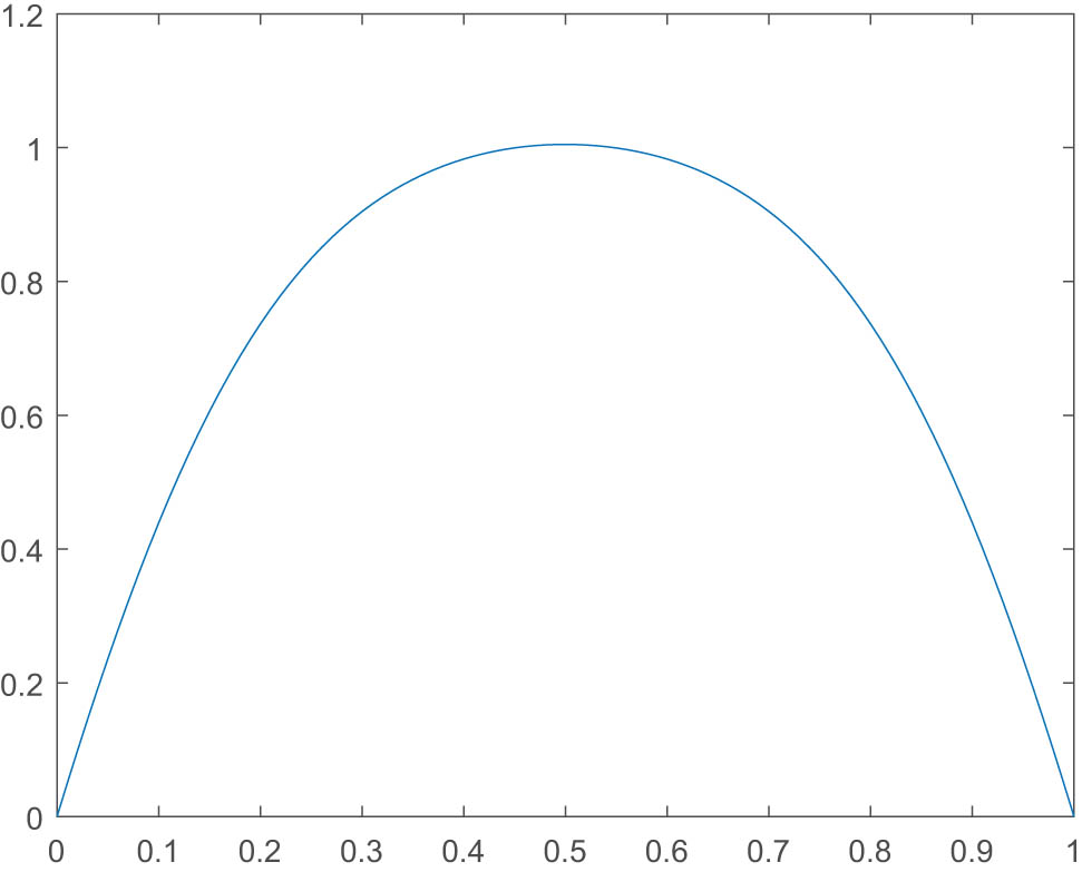
Solution
7 A primal dual variational formulation for a Burger’s type equation
In this section, we develop a primal dual variational formulation for a Burger’s type equation.
Let
Consider the Burger’s type equation in
where
At this point, we define the functional
Here,
Observe that
and denoting
Therefore,
Observe that at a critical point, we have
From this and (44), we may infer that
Thus, we may also conclude that the functional
7.1 A numerical example concerning a Burger’s type equation
In this subsection, we present numerical results related to a solution of the one-dimensional Burger’s equation:
with the boundary conditions
For a first example, we set
To obtain the numerical results, we have used an adaptation with small changes of the primal dual variational formulation presented in the previous section.
For the solution

Solution
For the case in which

Solution
Here, we present the software in MAT-LAB through which we have obtained such numerical results.
We highlight to have searched for a critical point of the primal dual formulation previously presented with some small changes and adaptations. Indeed, we have developed a procedure similar to the matrix version of the generalized method of lines.
Here, the software in a finite difference context, where
***********
1. clear all
m8=100;
d=1/m8;
K=5.0;
A=0.5;
for i=1:m8
uo(i,1)=1.0;
u1(i,1)=1.0;
v3(i,1)=K*uo(i,1);
end;
k2=1;
b14=1.0;
while
k2=k2+1;
k1=1;
b12=1.0;
while
k1=k1+1;
i=1;
m12=A*2+uo(i,1)*d+K*
m50(i)=A/m12;
z(i)=1/m12*(A+v3(i,1)*
for i=2:m8-1
m12=A*2-A*m50(i-1)+uo(i,1)*d-uo(i,1)*m50(i-1)*d+K*
m50(i)=A/m12;
z(i)=1/m12*(v3(i,1)*
end;
u(m8,1)=0.0;
for i=1:m8-1
u(m8-i,1)=m50(m8-i)*u(m8-i+1,1)+z(m8-i);
end;
b12=max(abs(u-uo));
uo=u;
end;
b14=max(abs(u-u1));
u1=u;
for i=1:m8-1
v3(i,1)=K*u(i,1);
end;
uo(50,1)
end;
for i=1:m8
x(i)=i*d;
end;
plot(x,u)
8 A primal dual variational formulation for a Navier–Stokes system
In this section, we develop a primal dual variational formulation for the time-independent incompressible Navier–Stokes system.
Consider
About the references, we emphasize that related existence, numerical, and theoretical results for similar systems may be found in [17–21], respectively. In particular, Temam [21] addresses extensively both theoretical and numerical methods and an interesting interplay between them.
Finally, these two first paragraphs of this article have been published as a preprint [22], more specifically, reference:
F.S. Botelho, Approximate Numerical Procedures for the Navier–Stokes System Through the Generalized Method of Lines. Preprints.org 2023, 2023020422.
https://doi.org/10.20944/preprints202302.0422.v3.
Defining now
As previously mentioned, at first, we look for solutions
At this point, we define the functional
and
Here,
We define also
and
so that
Observe that
and denoting
Therefore, defining
we have
Similarly, we may obtain
and denoting
Therefore, defining
we have
Moreover, we may have
Therefore, defining
we have
Finally, joining the pieces, we may infer that
Observe that at a critical point we have
and
From this and (44), we may infer that
Thus, we may also conclude that the functional
9 A duality principle for a related relaxed formulation concerning the vectorial approach in the calculus of variations
In this section, we develop a duality principle for a related vectorial model in the calculus of variations.
Let
For
where
and
We assume
Also
where
We define also
where
and
Moreover, we define the relaxed functional
where
Now observe that
Here, we have denoted
where
Furthermore,
Therefore, denoting
we obtain
Finally, we highlight such a dual functional
10 Conclusion
In this article, we have developed convex dual and primal dual variational formulations suitable for the local optimization of non-convex primal formulations.
It is worth highlighting, the results may be applied to a large class of models in physics and engineering.
We also emphasize that the first duality principles here presented are applied to a Ginzburg–Landau type equation. In particular, we highlight the primal dual formulation presented in Section 5, which is suitable for the global optimization of a originally nonconvex primal formulation.
Among the results, we have included primal dual variational formulations for a Burger’s type equation and for a time independent incompressible Navier–Stokes system. Concerning the Burger’s equation model, we have presented numerical examples and a related software in MAT-LAB.
Finally, in the last section, we have developed a new duality principle suitable for the relaxed quasi-convex primal formulation for a general model in a vectorial calculus of variations context.
In a future research, we intend to extend such results for some models of plates and shells and other models in the elasticity theory.
-
Funding information: The author states no funding involved.
-
Author contributions: The author has accepted responsibility for the entire content of this manuscript and approved its submission.
-
Conflict of interest: The author declares no conflict of interest concerning this article.
-
Data availability statement: Details on the software for numerical results available upon request.
References
[1] Bielski WR, Galka A, Telega JJ. The complementary energy principle and duality for geometrically nonlinear elastic shells. I. Simple case of moderate rotations around a tangent to the middle surface. Bulletin Polish Academy Sci Tech Sci. 1988;38:7–9. Search in Google Scholar
[2] Bielski WR, Telega JJ. A contribution to contact problems for a class of solids and structures. Arch Mech. 1985;37(4–5):303–20, Warszawa. Search in Google Scholar
[3] Telega JJ. On the complementary energy principle in non-linear elasticity. Part I: Von Karman plates and three dimensional solids. C.R. Acad Sci Paris Serie II. 1989;308:1193–8; Part II: Linear elastic solid and non-convex boundary condition. Minimax approach, ibid: 1313–1317. Search in Google Scholar
[4] Galka A, Telega JJ. Duality and the complementary energy principle for a class of geometrically non-linear structures. Part I. Five parameter shell model; Part II. Anomalous dual variational priciples for compressed elastic beams. Arch Mech. 1995;47:677–98, 699–724. Search in Google Scholar
[5] Toland JF. A duality principle for non-convex optimisation and the calculus of variations. Arch Rat Mech Anal. 1979;71(1):41–61. 10.1007/BF00250669Search in Google Scholar
[6] Adams RA, Fournier JF. Sobolev spaces, 2nd ed. New York (NY), USA: Elsevier; 2003. Search in Google Scholar
[7] Botelho F. Functional analysis and applied optimization in Banach spaces. Cham, Switzerland: Springer; 2014. 10.1007/978-3-319-06074-3Search in Google Scholar
[8] Botelho FS. Variational convex analysis [dissertation]. Blacksburg (VA): Virginia Tech; 2009. Search in Google Scholar
[9] Botelho F. Topics on functional analysis, calculus of variations and duality. Sofia, Bulgaria: Academic Publications; 2011. Search in Google Scholar
[10] Botelho F. Existence of solution for the Ginzburg–Landau system, a related optimal control problem and its computation by the generalized method of lines. Appl Math and Comp. 2012;218:11976–8910.1016/j.amc.2012.05.067Search in Google Scholar
[11] Rockafellar RT. Convex analysis. Princeton (NJ), USA: Princeton University Press; 1970. Search in Google Scholar
[12] Botelho FS. Functional analysis, calculus of variations and numerical methods in physics and engineering. Boca Raton (FL), USA: CRC Taylor and Francis; 2020. 10.1201/9780429343315Search in Google Scholar
[13] Botelho FS. Dual variational formulations for a large class of non-convex models in the calculus of variations. Mathematics. 2023;11(1):63. 10.3390/math11010063. Search in Google Scholar
[14] Annet JF. Superconductivity, superfluids and condensates. 2nd edn. Oxford Master Series in Condensed Matter Physics. Oxford, UK: Oxford University Press; 2010 Reprint. Search in Google Scholar
[15] Landau LD. Course of theoretical physics. Vol. 5. Statistical physics, part 1. Oxford, UK: Butterworth-Heinemann; 2008 Reprint.Search in Google Scholar
[16] Strikwerda JC. Finite difference schemes and partial differential equations. 2nd edition. Philadelphia (PA), USA: SIAM; 2004. 10.1137/1.9780898717938Search in Google Scholar
[17] Constantin P, Foias C. Navier–Stokes equation. Chicago (IL), USA: University of Chicago Press; 1989. 10.7208/chicago/9780226764320.001.0001Search in Google Scholar
[18] Hamouda M, Han D, Jung C-Y, Temam R. Boundary layers for the 3D primitive equations in a cube: the zero-mode. J Appl Anal Comp. 2018;8(3):873–89. 10.11948/2018.873. Search in Google Scholar
[19] Giorgini A, Miranville A, Temam R. Uniqueness and regularity for the Navier–Stokes-Cahn-Hilliard system. SIAM J Math Analysis (SIMA). 2019;51(3):2535–74. 10.1137/18M1223459. Search in Google Scholar
[20] Foias C, Rosa RM, Temam R. Properties of stationary statistical solutions of the three-dimensional Navier–Stokes equations. J Dynam Differ Equ. Special issue in memory of George Sell. 2019;31(3):1689–741. 10.1007/s10884-018-9719-2. Search in Google Scholar
[21] Temam R. Navier–Stokes equations. New York (NY), USA: Chelsea Publishing Company; 2001 Reprint.10.1090/chel/343Search in Google Scholar
[22] Botelho FS. Approximate numerical procedures for the Navier–Stokes system through the generalized method of lines. Preprints.org; 2023. p. 2023020422. 10.20944/preprints202302.0422.v3. [Preprint]Search in Google Scholar
© 2023 the author(s), published by De Gruyter
This work is licensed under the Creative Commons Attribution 4.0 International License.
Articles in the same Issue
- Research Articles
- The regularization of spectral methods for hyperbolic Volterra integrodifferential equations with fractional power elliptic operator
- Analytical and numerical study for the generalized q-deformed sinh-Gordon equation
- Dynamics and attitude control of space-based synthetic aperture radar
- A new optimal multistep optimal homotopy asymptotic method to solve nonlinear system of two biological species
- Dynamical aspects of transient electro-osmotic flow of Burgers' fluid with zeta potential in cylindrical tube
- Self-optimization examination system based on improved particle swarm optimization
- Overlapping grid SQLM for third-grade modified nanofluid flow deformed by porous stretchable/shrinkable Riga plate
- Research on indoor localization algorithm based on time unsynchronization
- Performance evaluation and optimization of fixture adapter for oil drilling top drives
- Nonlinear adaptive sliding mode control with application to quadcopters
- Numerical simulation of Burgers’ equations via quartic HB-spline DQM
- Bond performance between recycled concrete and steel bar after high temperature
- Deformable Laplace transform and its applications
- A comparative study for the numerical approximation of 1D and 2D hyperbolic telegraph equations with UAT and UAH tension B-spline DQM
- Numerical approximations of CNLS equations via UAH tension B-spline DQM
- Nonlinear numerical simulation of bond performance between recycled concrete and corroded steel bars
- An iterative approach using Sawi transform for fractional telegraph equation in diversified dimensions
- Investigation of magnetized convection for second-grade nanofluids via Prabhakar differentiation
- Influence of the blade size on the dynamic characteristic damage identification of wind turbine blades
- Cilia and electroosmosis induced double diffusive transport of hybrid nanofluids through microchannel and entropy analysis
- Semi-analytical approximation of time-fractional telegraph equation via natural transform in Caputo derivative
- Analytical solutions of fractional couple stress fluid flow for an engineering problem
- Simulations of fractional time-derivative against proportional time-delay for solving and investigating the generalized perturbed-KdV equation
- Pricing weather derivatives in an uncertain environment
- Variational principles for a double Rayleigh beam system undergoing vibrations and connected by a nonlinear Winkler–Pasternak elastic layer
- Novel soliton structures of truncated M-fractional (4+1)-dim Fokas wave model
- Safety decision analysis of collapse accident based on “accident tree–analytic hierarchy process”
- Derivation of septic B-spline function in n-dimensional to solve n-dimensional partial differential equations
- Development of a gray box system identification model to estimate the parameters affecting traffic accidents
- Homotopy analysis method for discrete quasi-reversibility mollification method of nonhomogeneous backward heat conduction problem
- New kink-periodic and convex–concave-periodic solutions to the modified regularized long wave equation by means of modified rational trigonometric–hyperbolic functions
- Explicit Chebyshev Petrov–Galerkin scheme for time-fractional fourth-order uniform Euler–Bernoulli pinned–pinned beam equation
- NASA DART mission: A preliminary mathematical dynamical model and its nonlinear circuit emulation
- Nonlinear dynamic responses of ballasted railway tracks using concrete sleepers incorporated with reinforced fibres and pre-treated crumb rubber
- Two-component excitation governance of giant wave clusters with the partially nonlocal nonlinearity
- Bifurcation analysis and control of the valve-controlled hydraulic cylinder system
- Engineering fault intelligent monitoring system based on Internet of Things and GIS
- Traveling wave solutions of the generalized scale-invariant analog of the KdV equation by tanh–coth method
- Electric vehicle wireless charging system for the foreign object detection with the inducted coil with magnetic field variation
- Dynamical structures of wave front to the fractional generalized equal width-Burgers model via two analytic schemes: Effects of parameters and fractionality
- Theoretical and numerical analysis of nonlinear Boussinesq equation under fractal fractional derivative
- Research on the artificial control method of the gas nuclei spectrum in the small-scale experimental pool under atmospheric pressure
- Mathematical analysis of the transmission dynamics of viral infection with effective control policies via fractional derivative
- On duality principles and related convex dual formulations suitable for local and global non-convex variational optimization
- Study on the breaking characteristics of glass-like brittle materials
- The construction and development of economic education model in universities based on the spatial Durbin model
- Homoclinic breather, periodic wave, lump solution, and M-shaped rational solutions for cold bosonic atoms in a zig-zag optical lattice
- Fractional insights into Zika virus transmission: Exploring preventive measures from a dynamical perspective
- Rapid Communication
- Influence of joint flexibility on buckling analysis of free–free beams
- Special Issue: Recent trends and emergence of technology in nonlinear engineering and its applications - Part II
- Research on optimization of crane fault predictive control system based on data mining
- Nonlinear computer image scene and target information extraction based on big data technology
- Nonlinear analysis and processing of software development data under Internet of things monitoring system
- Nonlinear remote monitoring system of manipulator based on network communication technology
- Nonlinear bridge deflection monitoring and prediction system based on network communication
- Cross-modal multi-label image classification modeling and recognition based on nonlinear
- Application of nonlinear clustering optimization algorithm in web data mining of cloud computing
- Optimization of information acquisition security of broadband carrier communication based on linear equation
- A review of tiger conservation studies using nonlinear trajectory: A telemetry data approach
- Multiwireless sensors for electrical measurement based on nonlinear improved data fusion algorithm
- Realization of optimization design of electromechanical integration PLC program system based on 3D model
- Research on nonlinear tracking and evaluation of sports 3D vision action
- Analysis of bridge vibration response for identification of bridge damage using BP neural network
- Numerical analysis of vibration response of elastic tube bundle of heat exchanger based on fluid structure coupling analysis
- Establishment of nonlinear network security situational awareness model based on random forest under the background of big data
- Research and implementation of non-linear management and monitoring system for classified information network
- Study of time-fractional delayed differential equations via new integral transform-based variation iteration technique
- Exhaustive study on post effect processing of 3D image based on nonlinear digital watermarking algorithm
- A versatile dynamic noise control framework based on computer simulation and modeling
- A novel hybrid ensemble convolutional neural network for face recognition by optimizing hyperparameters
- Numerical analysis of uneven settlement of highway subgrade based on nonlinear algorithm
- Experimental design and data analysis and optimization of mechanical condition diagnosis for transformer sets
- Special Issue: Reliable and Robust Fuzzy Logic Control System for Industry 4.0
- Framework for identifying network attacks through packet inspection using machine learning
- Convolutional neural network for UAV image processing and navigation in tree plantations based on deep learning
- Analysis of multimedia technology and mobile learning in English teaching in colleges and universities
- A deep learning-based mathematical modeling strategy for classifying musical genres in musical industry
- An effective framework to improve the managerial activities in global software development
- Simulation of three-dimensional temperature field in high-frequency welding based on nonlinear finite element method
- Multi-objective optimization model of transmission error of nonlinear dynamic load of double helical gears
- Fault diagnosis of electrical equipment based on virtual simulation technology
- Application of fractional-order nonlinear equations in coordinated control of multi-agent systems
- Research on railroad locomotive driving safety assistance technology based on electromechanical coupling analysis
- Risk assessment of computer network information using a proposed approach: Fuzzy hierarchical reasoning model based on scientific inversion parallel programming
- Special Issue: Dynamic Engineering and Control Methods for the Nonlinear Systems - Part I
- The application of iterative hard threshold algorithm based on nonlinear optimal compression sensing and electronic information technology in the field of automatic control
- Equilibrium stability of dynamic duopoly Cournot game under heterogeneous strategies, asymmetric information, and one-way R&D spillovers
- Mathematical prediction model construction of network packet loss rate and nonlinear mapping user experience under the Internet of Things
- Target recognition and detection system based on sensor and nonlinear machine vision fusion
- Risk analysis of bridge ship collision based on AIS data model and nonlinear finite element
- Video face target detection and tracking algorithm based on nonlinear sequence Monte Carlo filtering technique
- Adaptive fuzzy extended state observer for a class of nonlinear systems with output constraint