Dynamical aspects of transient electro-osmotic flow of Burgers' fluid with zeta potential in cylindrical tube
-
Nauman Raza


Abstract
In this article, we consider the flow of a Burgers’ fluid of transient electro-osmotic type in a small tube with a circular cross-section. Analytical results are found for the transient velocity and, electric potential profile by solving the Navier–Stokes and the linearized Poisson–Boltzmann equations. Moreover, these equations are solved with the help of the integral transform method. We consider cases in which the velocity of the fluid changes with time and those in which the velocity of the fluid does not change with time. Furthermore, special results for classical fluids such as Newtonian, second grade, Maxwell, and Oldroyd-B fluids are obtained as the particular cases of the outcomes of this work and that these results actually strengthen the results of the solution. This study of the nonlinear problem of Burgers’ fluid in a specified physical model will help us to understand the behavior of blood clotting and the block of any kind of problem in which this type of fluid is used. The solution of the complex velocity profile of Burgers’ fluid will help us in the future to solve the problems in which this transient electro-osmotic type of small tube is involved. At the end, numerical results are shown graphically that can help us to understand the complex behavior of the Burgers’ fluid, and also the analysis of the Burgers’ fluid shows dissimilarity with other fluids that are considered in this work.
| Nomenclature | ||
|---|---|---|
| Physical quantity | Symbol | SI units |
| Velocity vector |
|
|
| Force vector of the external body |
|
N |
| Cauchy stress tensor |
|
|
| Fluid density |
|
|
| Unit tensor |
|
— |
| Extra stress tensor |
|
|
| Dynamic viscosity |
|
|
| Pressure |
|
|
| Tensor transpose |
|
— |
| Relaxation time |
|
s |
| New material parameter |
|
|
| Retardation time |
|
s |
| Circular tube radius |
|
m |
| Time |
|
s |
| Dielectric constant |
|
— |
| Zeta potential on tube wall |
|
|
| Outer electric field |
|
|
| Component of velocity field |
|
|
| Potential distribution |
|
V |
| Net charge density |
|
|
| Valence of ion |
|
— |
| Fundamental charge |
|
C |
| Boltzmann constant |
|
|
| Absolute temperature |
|
K |
| Electric double layer (EDL) thickness |
|
m |
| Debye–Hückel parameter |
|
— |
| Zero order modified bessel function |
|
— |
| Bessel function of first kind |
|
— |
| Radial coordinate |
|
m |
1 Introduction
Recently, electro-osmotic flow (EOF) has become a more attractive topic in microfluid because of its operational advantages such as high reliability, better control flow, and low noise, and has found applications in the majority of fields such as biological analyses, chemical, and medical diagnoses. On the basis of the study of EOF, several authors attract our attention to the non-Newtonian fluid [1–3]. Many significant contributions such as articles and books are published in the literature. The first book about electro-osmosis of polymer solutions [4] was published in 2017. Furthermore, many research articles in the literature have been published to discuss electro-osmosis flow. We only discuss and cited those article that is nearly related to our research work.
Many researchers have shown great interest in electrokinetic microflows of non-Newtonian biofluids. The impact of EOF in the field of non-Newtonian fluids was first studied by Das and Chakraborty [5,6]. In their study, the non-Newtonian flow of a fluid in a rectangular small channel is affected by electrokinetic influences. For a similar model of non-Newtonian fluid, Zhao and Yang [7,8] derive the generalized Smoluchowski velocity with zeta random potential over a surface for electro-osmosis. Bandopadhyay and Chakraborty [9] impart the dynamical interchange between consolidated dissipative and elastic conduct of restricted flow by using Fourier transform. They proposed that the variability of EOF is affected by the size of both the ions and the channel. Wang and Zhao [10] introduced the solution of a generalized Maxwell fluid flow of transient electro-osmotic type with fractional derivative in a narrow capillary tube. After the study of this technique, Zhao et al. [11] analyzed the EOF of Oldroyd-B fluid through cylindrical geometry and obtained the solution with the help of an integral transform method. Most research work in EOF is the state of steady flow [12,13]. Berg and Ladipo [14] studied the flow problem with unlimited cylindrical pores in a surface of uniform charge density. Chang [15] studied the flow of transient EOF containing the salt-free medium by a cylindrical microcapillary for both constant potential surface and constant charge surface, and the exact solution of transient EOF velocity field and the potential electric distribution was computed by using the nonlinear Navier–Stokes and the Poisson–Boltzmann equations. The model of EOF flows with the application of a stepwise voltage in a broad capillary, and both aperiodical and periodical flow schemes were inspected by Mishchuk and Gonzlez-Caballero [16]. Some of the authors recently also studied the mass transport process of different fluid flows under magnetic effects [17,18]. We have studied the dynamic aspect of transient electro-osmotic flow with zeta potential combined in the same model, but before this, these models were studied separately as just traveling waves [19,20], dynamic aspects of some biological models [21], or in the thermal conductance of nanofluids [22].
In this article, the non-Newtonian behavior of biofluids is modeled by the Burgers’ constitutive equation, and then we find the analytical results for the electric potential and transient velocity profile by solving the linearized Poisson–Boltzmann and Navier–Stokes equations. Moreover, these equations are solved with the help of the integral transform technique. The motivation behind this work is to find the solution of the unsteady electro-osmotic flow of Burger fluid in a circular cross-sectional tube.
2 Mathematical modeling of the problem
The continuity equation for a fluid of constant density is
and the equation of Cauchy momentum (C.M) in general form is
where
where
This model incorporates the Oldroyd-B display (for
Consider a straight tube with a circular cross-section of radius
We will use polar coordinates
with initial condition
and the condition given in Eq. (1) is fulfilled naturally.
As indicated by the theory of electrostatics, the relationship between the potential distribution
On the tube wall, the boundary condition is the zeta potential
In the present investigation, the charge dispersion is not influenced by
where the initial and boundary conditions are as follows:
3 Exact solution for the model
Considering the limited ionic size, we ignore all nonelectro-static connections between the ions, i.e., here we consider the particles to be point sized. For of
where
By using the approximation of the Debye–Hückel, [23,24], Eq. (9) is linearized as follows:
Eq. (11) becomes
here,
Removing
The nondimensional parameters are as follows:
By substituting the aforementioned standardized factors into Eqs. (15) and (18) and also the conditions of initial and boundary (10), (12), and (13) results in (for ease of reading, the nondimensional symbol “
where
and
The solution of Eqs. (20) and (24) is
Here,
and the inverse Laplace and inverse Hakel transforms
where the zero-order
Now, we discuss a special case for
Eq. (32) becomes
We can find the analytical solution by using inverse Laplace and inverse Hankel transforms:
where
and
where
4 Particular cases
4.1 Oldroyd-B fluid
4.1.1 With pressure gradient
Burgers’ fluid becomes Oldroyd-B, when
where
also
and
4.1.2 Without pressure gradient
The particular kind of the Burger fluid with
where
4.2 Maxwell fluid
4.2.1 With pressure gradient
The solution for a Maxwell fluid is obtained by introducing
where
and
Also,
and
4.2.2 Without pressure gradient
The solution for a Maxwell fluid is obtained by introducing
where
4.3 Second grade fluid
4.3.1 With pressure gradient
When
where
It is important to mentioned that the value of
4.3.2 Without pressure gradient
When
4.4 Newtonian fluid
4.4.1 With pressure gradient
By using
or
4.4.2 Without pressure gradient
Burgers’ fluid with
or
The outcomes of Kang et al. [25] are similar to Eq. (52) by utilizing the technique of Green’s function. In this article the advantage of the solution is the effortlessness of Eq. (52), in which we consider the steady part as follows:
with the outcome given by Rice and Whitehead [26], and the rest is the unsteady one.
5 Numerical results and discussion
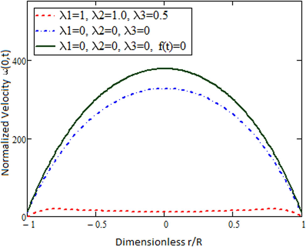
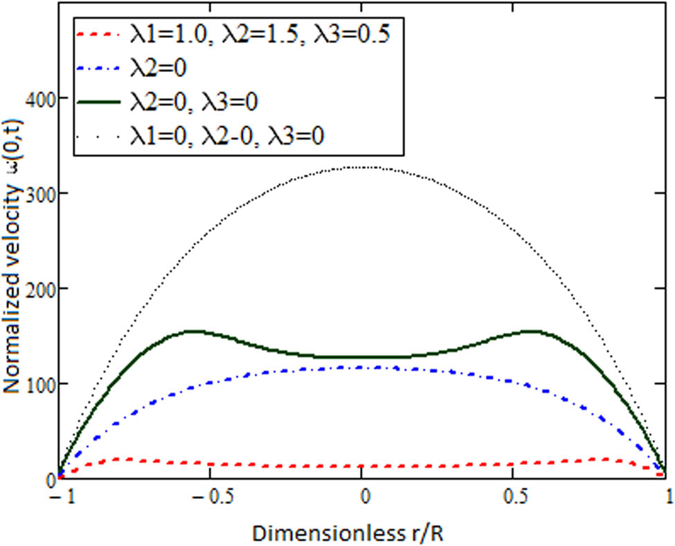
To illustrate some physically interesting aspects of the derived results, the normalized velocity
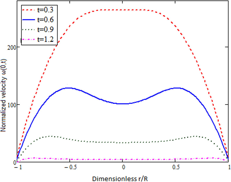
In the pipe behavior of flow when
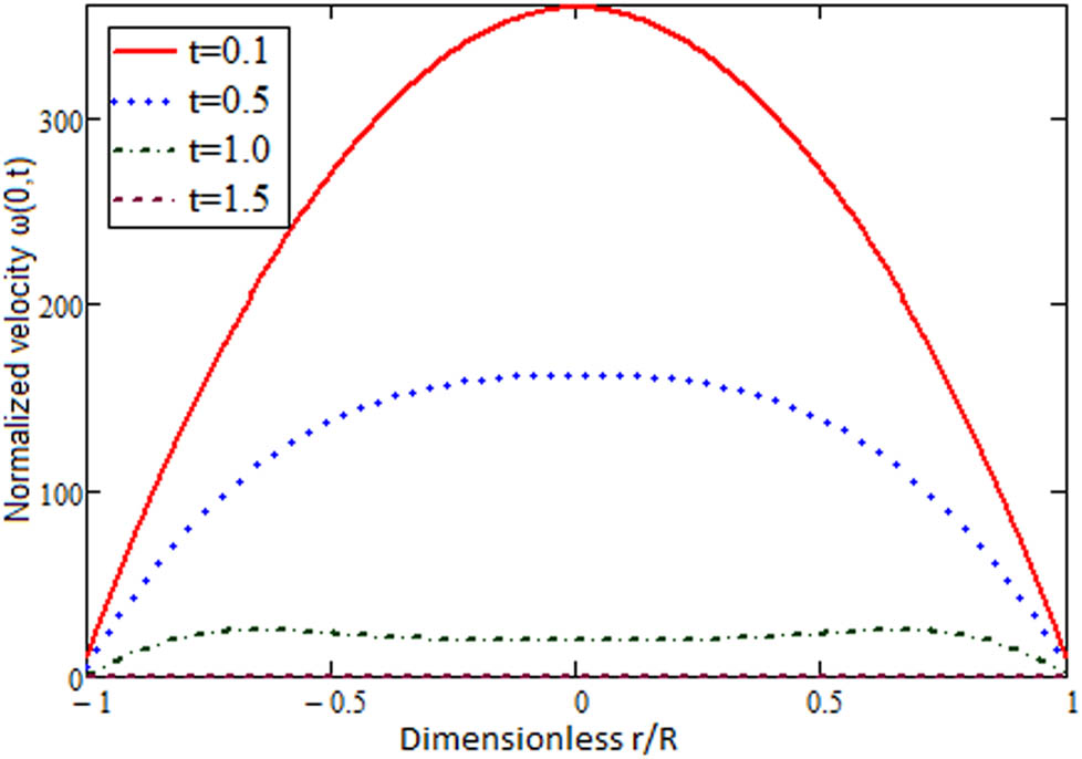
In the pipe behavior of flow when
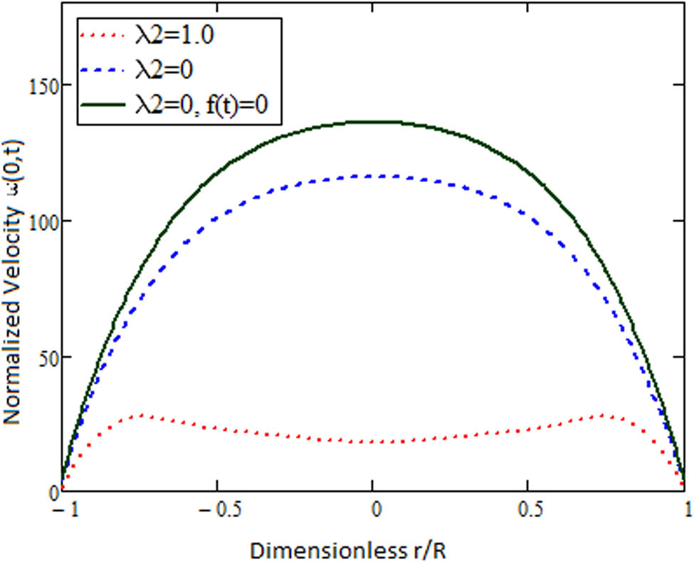
Comparative behavior of Oldroyd-B fluid (with
Comparative behavior of Maxwell fluid (with
Comparative behavior of the Newtonian fluid (with
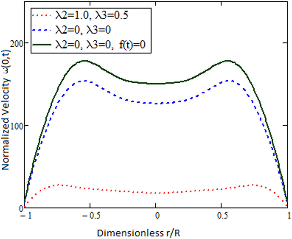
Comparative behavior of Oldroyd-B, Maxwell, Newtonian, and Burgers’ fluids.
6 Conclusion
The analytical solutions for the transient flow of a Burgers’ fluid in a small cross-section tube of electro-osmotic type with Debye–Hückel approximation have obtained in this work. Poisson–Boltzmann and the Navier–Stokes linearized equations are solved to obtain the analytical results for electric potential
Acknowledgments
Dr. Kashif Ali Abro is highly thankful and grateful to Mehran University of Engineering and Technology, Jamshoro, Pakistan, for generous support and facilities of this research work.
-
Funding information: The author states no funding involved.
-
Author contributions: All author has accepted responsibility for the entire content of this manuscript and approved its submission.
-
Conflict of interest: The authors state no conflict of interest.
References
[1] Sadeghi V, Baheri S, Arsalani N. An experimental investigation of the effect of using non-Newtonian nanofluid-graphene oxide/aqueous solution of sodium carboxymethyl cellulose-on the performance of direct absorption solar collector. Sci Iran. 2020;28(3):1284–97. 10.24200/sci.2020.54994.4024Suche in Google Scholar
[2] Rizwan M, Hassan M, Makinde OD, Bhatti MM, Marin M. Rheological modeling of metallic oxide nanoparticles containing non-newtonian nanofluids and potential investigation of heat and mass flow characteristics. Nanomaterials. 2022;12(7):1237. 10.3390/nano12071237Suche in Google Scholar PubMed PubMed Central
[3] Bhatti MM, Zeeshan A, Bashir F, Sait SM, Ellahi R. Sinusoidal motion of small particles through a Darcy-Brinkman-Forchheimer microchannel filled with non-Newtonian fluid under electro-osmotic forces. J Taibah Univ Sci. 2021;15(1):514–29.10.1080/16583655.2021.1991734Suche in Google Scholar
[4] Uematsu Y. Electro-osmosis of polymer solutions: linear and nonlinear behavior. Singapore: Springer; 2017. 10.1007/978-981-10-3424-4Suche in Google Scholar
[5] Das S, Chakraborty S. Analytical solutions for velocity, temperature and concentration distribution in electroosmotic microchannel flows of a non-Newtonian bio-fluid. Anal Chim Acta. 2006;559(1):15–24. 10.1016/j.aca.2005.11.046Suche in Google Scholar
[6] Chakraborty S. Electro osmotically driven capillary transport of typical non-Newtonian biofluids in rectangular microchannels. Anal Chim Acta. 2007;605(2):175–84. 10.1016/j.aca.2007.10.049Suche in Google Scholar PubMed
[7] Zhao C, Yang C. Exact solutions for electro-osmotic flow of viscoelastic fluids in rectangular micro-channels. Appl Math Comput. 2009;211(2):502–9. 10.1016/j.amc.2009.01.068Suche in Google Scholar
[8] Zhao C, Yang C. Nonlinear Smoluchowski velocity for electroosmosis of Power-law fluids over a surface with arbitrary zeta potentials. Electrophoresis 2010;31(5):973–9. 10.1002/elps.200900564Suche in Google Scholar PubMed
[9] Bandopadhyay A, Chakraborty S. Electro kinetically induced alterations in dynamic response of visco elastic fluids in narrow confinements. Phys Rev E. 2012;85(5):056302. 10.1103/PhysRevE.85.056302Suche in Google Scholar PubMed
[10] Wang S, Zhao M. Analytical solution of the transient electro-osmotic flow of a generalized fractional Maxwell fluid in a straight pipe with a circular cross-section. Eur J Mech B Fluids 2015;54:82–6. 10.1016/j.euromechflu.2015.06.016Suche in Google Scholar
[11] Zhao M, Wang S, Wei S. Transient electro-osmotic flow of Oldroyd-B fluids in a straight pipe of circular cross section. J Non-Newtonian Fluid Mech. 2013;201:135–9. 10.1016/j.jnnfm.2013.09.002Suche in Google Scholar
[12] Dhinakaran S, Afonso AM, Alves MA, Pinho FT. Steady viscoelastic fluid flow between parallel plates under electro-osmotic forces: Phan-Thien-Tanner model. J Colloid Interface Sci. 2010;344(2):513–20. 10.1016/j.jcis.2010.01.025Suche in Google Scholar PubMed
[13] Horiuchi K, Dutta P. Joule heating effects in electroosmotically driven microchannel flows. Int J Heat Mass Transfer. 2004;47(14-16):3085–95. 10.1016/j.ijheatmasstransfer.2004.02.020Suche in Google Scholar
[14] Berg P, Ladipo K. Exact solution of an electro-osmotic flow problem in a cylindrical channel of polymer electrolyte membranes. Proc R Soc A Math Phys Eng Sci. 2009;465(2109):2663–79. 10.1098/rspa.2009.0067Suche in Google Scholar
[15] Chang SH. Transient electro-osmotic flow in cylindrical microcapillaries containing salt-free medium. Biomicrofluidics. 2009;3(1):012802. 10.1063/1.3064113Suche in Google Scholar PubMed PubMed Central
[16] Mishchuk NA, Gonzlez-Caballero F. Nonstationary electro osmotic flow in open cylindrical capillaries. Electrophoresis. 2006;27(3):650–60. 10.1002/elps.200500470Suche in Google Scholar PubMed
[17] Bhatti MM, Jun S, Khalique CM, Shahid A, Fasheng L, Mohamed MS. Lie group analysis and robust computational approach to examine mass transport process using Jeffrey fluid model. Appl Math Comput. 2022;421:126936. 10.1016/j.amc.2022.126936Suche in Google Scholar
[18] Bhatti MM, Zeeshan A, Asif MA, Ellahi R, Sait SM. Non-uniform pumping flow model for the couple stress particle-fluid under magnetic effects. Chem Eng Commun. 2021;209(8):1058–69. 10.1080/00986445.2021.1940156Suche in Google Scholar
[19] Durur H, Yokuş A, Abro KA. Computational and traveling wave analysis of Tzitzéica and Dodd-Bullough-Mikhailov equations: an exact and analytical study. Nonlinear Eng. 2021;10(1):272–81. 10.1515/nleng-2021-0021Suche in Google Scholar
[20] Yokuş A, Durur H, Abro KA. Role of shallow water waves generated by modified Camassa-Holm equation: a comparative analysis for traveling wave solutions. Nonlinear Eng. 2021;10(1):385–94. 10.1515/nleng-2021-0030Suche in Google Scholar
[21] Awan AU, Sharif A, Abro KA, Ozair M, Hussain T. Dynamical aspects of smoking model with cravings to smoke. Nonlinear Eng. 2021;10(1):91–108. 10.1515/nleng-2021-0008Suche in Google Scholar
[22] Panhwer LA, Abro KA, Memon IQ. Thermal deformity and thermolysis of magnetized and fractional Newtonian fluid with rheological investigation. Phys Fluids. 2022;34(5):053115. 10.1063/5.0093699Suche in Google Scholar
[23] Krishnan M, J, Rajagopal KR. Review of the uses and modeling of bitumen from ancient to modern times. Appl Mech Rev. 2003;56(2):149–214. 10.1115/1.1529658Suche in Google Scholar
[24] Masliyah JH, Bhattacharjee S. Electrokinetic and colloid transport phenomena. Hoboken, New Jersey: John Wiley and Sons; 2006. 10.1002/0471799742Suche in Google Scholar
[25] Kang Y, Yang C, Huang X. Dynamic aspects of electroosmotic flow in a cylindrical microcapillary. Int J Eng Sci. 2002;40(20):2203–21. 10.1016/S0020-7225(02)00143-XSuche in Google Scholar
[26] Rice CL, Whitehead R. Electro kinetic flow in a narrow cylindrical capillary. J Phys Chem. 1965;69(11):4017–24. 10.1021/j100895a062Suche in Google Scholar
[27] Stehfest H. Algorithm 368: numerical inversion of Laplace transforms [D5]. Commun ACM. 1970;13(1):47–9. 10.1145/361953.361969Suche in Google Scholar
[28] Awan AU, Riaz S, Abro KA, Siddiqa A, Ali Q. The role of relaxation and retardation phenomenon of Oldroyd-B fluid flow through Stehfestas and Tzouas algorithms. Nonlinear Eng. 2022;11(1):35–46. 10.1515/nleng-2022-0006Suche in Google Scholar
© 2023 the author(s), published by De Gruyter
This work is licensed under the Creative Commons Attribution 4.0 International License.
Artikel in diesem Heft
- Research Articles
- The regularization of spectral methods for hyperbolic Volterra integrodifferential equations with fractional power elliptic operator
- Analytical and numerical study for the generalized q-deformed sinh-Gordon equation
- Dynamics and attitude control of space-based synthetic aperture radar
- A new optimal multistep optimal homotopy asymptotic method to solve nonlinear system of two biological species
- Dynamical aspects of transient electro-osmotic flow of Burgers' fluid with zeta potential in cylindrical tube
- Self-optimization examination system based on improved particle swarm optimization
- Overlapping grid SQLM for third-grade modified nanofluid flow deformed by porous stretchable/shrinkable Riga plate
- Research on indoor localization algorithm based on time unsynchronization
- Performance evaluation and optimization of fixture adapter for oil drilling top drives
- Nonlinear adaptive sliding mode control with application to quadcopters
- Numerical simulation of Burgers’ equations via quartic HB-spline DQM
- Bond performance between recycled concrete and steel bar after high temperature
- Deformable Laplace transform and its applications
- A comparative study for the numerical approximation of 1D and 2D hyperbolic telegraph equations with UAT and UAH tension B-spline DQM
- Numerical approximations of CNLS equations via UAH tension B-spline DQM
- Nonlinear numerical simulation of bond performance between recycled concrete and corroded steel bars
- An iterative approach using Sawi transform for fractional telegraph equation in diversified dimensions
- Investigation of magnetized convection for second-grade nanofluids via Prabhakar differentiation
- Influence of the blade size on the dynamic characteristic damage identification of wind turbine blades
- Cilia and electroosmosis induced double diffusive transport of hybrid nanofluids through microchannel and entropy analysis
- Semi-analytical approximation of time-fractional telegraph equation via natural transform in Caputo derivative
- Analytical solutions of fractional couple stress fluid flow for an engineering problem
- Simulations of fractional time-derivative against proportional time-delay for solving and investigating the generalized perturbed-KdV equation
- Pricing weather derivatives in an uncertain environment
- Variational principles for a double Rayleigh beam system undergoing vibrations and connected by a nonlinear Winkler–Pasternak elastic layer
- Novel soliton structures of truncated M-fractional (4+1)-dim Fokas wave model
- Safety decision analysis of collapse accident based on “accident tree–analytic hierarchy process”
- Derivation of septic B-spline function in n-dimensional to solve n-dimensional partial differential equations
- Development of a gray box system identification model to estimate the parameters affecting traffic accidents
- Homotopy analysis method for discrete quasi-reversibility mollification method of nonhomogeneous backward heat conduction problem
- New kink-periodic and convex–concave-periodic solutions to the modified regularized long wave equation by means of modified rational trigonometric–hyperbolic functions
- Explicit Chebyshev Petrov–Galerkin scheme for time-fractional fourth-order uniform Euler–Bernoulli pinned–pinned beam equation
- NASA DART mission: A preliminary mathematical dynamical model and its nonlinear circuit emulation
- Nonlinear dynamic responses of ballasted railway tracks using concrete sleepers incorporated with reinforced fibres and pre-treated crumb rubber
- Two-component excitation governance of giant wave clusters with the partially nonlocal nonlinearity
- Bifurcation analysis and control of the valve-controlled hydraulic cylinder system
- Engineering fault intelligent monitoring system based on Internet of Things and GIS
- Traveling wave solutions of the generalized scale-invariant analog of the KdV equation by tanh–coth method
- Electric vehicle wireless charging system for the foreign object detection with the inducted coil with magnetic field variation
- Dynamical structures of wave front to the fractional generalized equal width-Burgers model via two analytic schemes: Effects of parameters and fractionality
- Theoretical and numerical analysis of nonlinear Boussinesq equation under fractal fractional derivative
- Research on the artificial control method of the gas nuclei spectrum in the small-scale experimental pool under atmospheric pressure
- Mathematical analysis of the transmission dynamics of viral infection with effective control policies via fractional derivative
- On duality principles and related convex dual formulations suitable for local and global non-convex variational optimization
- Study on the breaking characteristics of glass-like brittle materials
- The construction and development of economic education model in universities based on the spatial Durbin model
- Homoclinic breather, periodic wave, lump solution, and M-shaped rational solutions for cold bosonic atoms in a zig-zag optical lattice
- Fractional insights into Zika virus transmission: Exploring preventive measures from a dynamical perspective
- Rapid Communication
- Influence of joint flexibility on buckling analysis of free–free beams
- Special Issue: Recent trends and emergence of technology in nonlinear engineering and its applications - Part II
- Research on optimization of crane fault predictive control system based on data mining
- Nonlinear computer image scene and target information extraction based on big data technology
- Nonlinear analysis and processing of software development data under Internet of things monitoring system
- Nonlinear remote monitoring system of manipulator based on network communication technology
- Nonlinear bridge deflection monitoring and prediction system based on network communication
- Cross-modal multi-label image classification modeling and recognition based on nonlinear
- Application of nonlinear clustering optimization algorithm in web data mining of cloud computing
- Optimization of information acquisition security of broadband carrier communication based on linear equation
- A review of tiger conservation studies using nonlinear trajectory: A telemetry data approach
- Multiwireless sensors for electrical measurement based on nonlinear improved data fusion algorithm
- Realization of optimization design of electromechanical integration PLC program system based on 3D model
- Research on nonlinear tracking and evaluation of sports 3D vision action
- Analysis of bridge vibration response for identification of bridge damage using BP neural network
- Numerical analysis of vibration response of elastic tube bundle of heat exchanger based on fluid structure coupling analysis
- Establishment of nonlinear network security situational awareness model based on random forest under the background of big data
- Research and implementation of non-linear management and monitoring system for classified information network
- Study of time-fractional delayed differential equations via new integral transform-based variation iteration technique
- Exhaustive study on post effect processing of 3D image based on nonlinear digital watermarking algorithm
- A versatile dynamic noise control framework based on computer simulation and modeling
- A novel hybrid ensemble convolutional neural network for face recognition by optimizing hyperparameters
- Numerical analysis of uneven settlement of highway subgrade based on nonlinear algorithm
- Experimental design and data analysis and optimization of mechanical condition diagnosis for transformer sets
- Special Issue: Reliable and Robust Fuzzy Logic Control System for Industry 4.0
- Framework for identifying network attacks through packet inspection using machine learning
- Convolutional neural network for UAV image processing and navigation in tree plantations based on deep learning
- Analysis of multimedia technology and mobile learning in English teaching in colleges and universities
- A deep learning-based mathematical modeling strategy for classifying musical genres in musical industry
- An effective framework to improve the managerial activities in global software development
- Simulation of three-dimensional temperature field in high-frequency welding based on nonlinear finite element method
- Multi-objective optimization model of transmission error of nonlinear dynamic load of double helical gears
- Fault diagnosis of electrical equipment based on virtual simulation technology
- Application of fractional-order nonlinear equations in coordinated control of multi-agent systems
- Research on railroad locomotive driving safety assistance technology based on electromechanical coupling analysis
- Risk assessment of computer network information using a proposed approach: Fuzzy hierarchical reasoning model based on scientific inversion parallel programming
- Special Issue: Dynamic Engineering and Control Methods for the Nonlinear Systems - Part I
- The application of iterative hard threshold algorithm based on nonlinear optimal compression sensing and electronic information technology in the field of automatic control
- Equilibrium stability of dynamic duopoly Cournot game under heterogeneous strategies, asymmetric information, and one-way R&D spillovers
- Mathematical prediction model construction of network packet loss rate and nonlinear mapping user experience under the Internet of Things
- Target recognition and detection system based on sensor and nonlinear machine vision fusion
- Risk analysis of bridge ship collision based on AIS data model and nonlinear finite element
- Video face target detection and tracking algorithm based on nonlinear sequence Monte Carlo filtering technique
- Adaptive fuzzy extended state observer for a class of nonlinear systems with output constraint