Convolutional neural network for UAV image processing and navigation in tree plantations based on deep learning
-
Shuiqing Xiao


Abstract
In this study, we show a new way for a small unmanned aerial vehicle (UAV) to move around on its own in the plantations of the tree using a single camera only. To avoid running into trees, a control plan was put into place. The detection model looks at the image heights of the trees it finds to figure out how far away they are from the UAV. It then looks at the widths of the image between the trees without any obstacles to finding the largest space. The purpose of this research is to investigate how virtual reality (VR) may improve student engagement and outcomes in the classroom. The emotional consequences of virtual reality on learning, such as motivation and enjoyment, are also explored, making this fascinating research. To investigate virtual reality’s potential as a creative and immersive tool for boosting educational experiences, the study adopts a controlled experimental method. This study’s most significant contributions are the empirical evidence it provides for the efficacy of virtual reality in education, the illumination of the impact VR has on various aspects of learning, and the recommendations it offers to educators on how to make the most of VR in the classroom.
1 Introduction
Unmanned aerial vehicles (UAVs) are aircraft that are without a pilot present to guide and direct them. The people on the ground can handle these flying vehicles from a distance, or they can be programmed to fly themselves. UAVs have been used in precision gardening because they are more flexible and able than labor-intensive methods. According to Lee et al. [1], UAVs have been utilized to take images from the air as well as obtain other critical information from the instruments on board. By analyzing the data gathered by UAVs, the task can be accomplished swiftly and well. These data help the farmers do several important jobs in the plantations, like analyzing and planning the farming, keeping an eye on the plantations, and then reporting on the state of health and development of the agricultural land through crop surveillance and soil analysis of samples. With the tools we have currently, UAVs can do precise farming tasks like tracking and keeping a watch on trees by flying at a height. At this altitude, they can see many things and can make superior observations [2]. They also have a lot of room to fly without any obstacles. But it takes more expensive devices or equipment to get data of good enough quality. Some jobs are also hard to do when you are far away. On the other hand, UAVs that can fly at low altitudes can do a lot of other jobs that are easier and cheaper to do. For example, they can keep a close eye on crops and spray fertilizer in the right amount based on how the land is doing. These UAVs may utilize a small camera to capture images of their targets, like dirt or crops when they are close by. Research design by Windrim et al. [3] shows that these pictures can then be used to analyze and process the data. Using UAVs at low altitudes is more efficient and saves money than sending people out to work in a large area. Convolutional Neural Network (CNN)-based navigation algorithms have difficulty in complicated environments like tree plantations because of occlusions, differences in a tree structure, and changes in illumination. They may be made more effective via the use of a number of different methods. Data augmentation approaches might be used as a first step in improving the network’s generalizability and capacity to manage variances in tree planting circumstances. Second, attention techniques may improve feature extraction efficiency and mitigate the effect of occlusions by focusing on just the important regions of the picture. In addition, preparing the network on big data sets with a variety of environmental factors may increase the network’s resilience and adaptability to challenging tree planting conditions through transfer learning.
But in a low-altitude flight, the biggest problem is keeping the UAV from crashing in a crowded area while it is exploring. Pilots with a lot of experience can see and dodge obstacles from live-stream videos or line-of-sight operations. But the plantation setting is hard for human pilots to handle because they have to do a lot of work. Also, it is very expensive to hire pilots with a lot of experience. According to Barbosa et al. [4], the robot must be able to detect and avoid obstacles autonomously. Using obstacle recognition methods, it is possible to locate objects in the environment. Based on what it knows about its surroundings, the flight controller makes an order to move the plane away from any obstacles it finds. So, it needs onboard sensors and control programs to find things and control how it moves.
Selvaraj et al. [5] found even though these ways can give accurate measurements, they can only see so far. The expense, large quantities, and energy consumption of these gadgets all limit the UAV’s efficiency. Because of its portability, lightweight, and low energy consumption, just one camera is preferable for obstacle avoidance.
Both motion-based and knowledge-based approaches exist for monocular obstacle identification. The depth of an object can be estimated by the use of the motion-based approach known as optical flow. According to Sandino et al. [6], “Dense optical flow,” the process of following every individual pixel between two consecutive picture frames, allows us to identify the source of motion. Due to the high data rate of the optical flow, a large amount of storage and processing power is required. One alternative is to look for landmarks in one image and then continue following those features into the next. This technique is superior, and it’s termed “sparse optical flow.” It is great for tiny UAVs. However, the image noise may make it difficult to figure out the obstruction. Knowledge-based solutions, such as machine learning or approaches that integrate with ocular flow methods, have been developed since monocular vision prevents precise and reliable distance measurement.
2 Literature review
According to Islam et al. [7], CNN has been successfully employed in recent years for picture object detection, segmentation, and identification. CNN-based approaches have been used to locate vehicles, medical pictures, and also fruits. Since Alexnet won the 2012 ImageNet competition, CNNs have been the defector method of choice when it comes to the classification of visual content. CNN’s approaches outperformed humans on the ImageNet task presented by Fichtel et al. [8].
According to Badrloo et al. [9], there have been several successful implementations of autonomous navigation using UAVs guided by monocular views. If you just have one eye, though, you won’t be able to gauge depth as well. There were just a few suggestions about how to improve UAV autonomous guiding in this situation. According to the research design by Badrloo et al. [9], reconstructing scenes from the UAV’s motion data is the goal of Structure from Motion (SfM) techniques. An established depth map was created from a limited number of successive photos and then utilized to create waypoints [10]. By enabling the creation of detailed depth visualizations in real-time and facilitating navigation in a congested outdoor scenario, direct depth estimation was proposed. However, the SfM-based obstacle-avoiding strategy cannot protect the UAV against moving targets that move while mapping or during mapping cycles. To gain depth information, the mapping cycles have to retain and compare the images of the location one after the other argued by Hao et al. [11].
According to Torres et al. [12], it is also possible to estimate depth using techniques based on optical flow. This technique was developed to obtain the depth of a picture in a 3D environment, and it is based on the gradient-based approach [13]. The model could determine the movement of the obstruction by comparing successive images. Using these data, the UAV was guided using an orientation strategy that is inversely related to the optical flow disparity between the left and right sides of the picture argued by Bhattacharyay et al. [14].
Research by Kadethankar et al. [15] explains that optical flow navigation strategies that take biological inspiration are also in the table. It was demonstrated that the longitudinal visual flow strategy used to achieve collision-free flight is inspired by the way insects navigate their environments. However, optical flow-based approaches may be less ideal since they cannot get precise distances. According to Apolo-Apolo et al. [16], a sophisticated process called SLAM, which stands for simultaneous localization and mapping, has been proposed as a means of creating precise metric maps. UAVs are better able to locate and avoid hazards thanks to the information gained via this technology. In most cases, information is provided by ultrasonic or IR range finders. It has been demonstrated that an SLAM system based on LiDAR can successfully guide UAVs across an interior environment [17].
According to Kulbacki et al. [18], combining data from LiDAR, GPS, and CNN-based algorithms ensures reliable navigation in tree plantations. The accurate depth data and 3D point cloud information provided by LiDAR allow the program to recognize intricate tree structures and handle occlusions. The updated information allows for improved object detection, depth estimation, and obstacle avoidance researched by Darwin et al. [19]. The program is able to traverse the plantation with pinpoint precision because of the global positioning and localization capabilities provided by GPS sensors. An effective navigation system capable of handling tree plantations is made possible by combining LiDAR, GPS, and algorithms based on CNNs [20].
According to Yu et al. [21], some strategies monitor the area ahead of the vehicle, adapting its path if an obstruction is detected. The term “sense-and-avoid” is commonly used to describe this approach. As part of a strategy, the UAV’s prior knowledge of the environment was utilized in conjunction with a classification approach to determine the environment type and the UAV’s flying path. Mumuni et al. [22] disclose that this technique was limited to non-commercial, domestic use. This was accomplished with the use of motion planning techniques for determining the optimal course of action in more intricate scenarios. Li et al. [23] proposed a technique using local path optimization along with learning from demonstrations to enhance the initial approaches for local optimization. The trained model did more than just avoid dangerous local minima; it also plotted a smooth path. Alternately, Coordinate conversion and the Kalman filter were then used to estimate the location and direction of the moving objects [24].
According to Yang et al. [25], a two-phase deep reinforcement learning approach to obstacle avoidance was proposed. Combining a fully CNN with a Double-Q Network (D3QN), this system achieved superior results. While the CNN forecasts depth, the D3QN predicts the Q-value of rotating activities with linear actions simultaneously using a network of convolutions and a dual network. Research by Meivel and Maheswari et al. [26] explains that a novel CNN architecture called Joint Monocular Obstacle Recognition (J-MOD2) was recently proposed to learn depth estimates and obstacle recognition using image data recovered via VGG19 fine-tuned model [27].
3 Methodology
The effectiveness of navigation algorithms used in tree plantations depends on selecting the correct CNN architecture. Popular choices include Res Net, VGG, and Efficient Net, all of which are able to gather hierarchical and discriminative features. The network’s capacity to learn complicated representations is a result of its depth, breadth, and the number of convolutional layers. The method of training and generalization ability are both influenced by hyper-parameters such as learning rate, number of batches, and weight decay. Using optimization methods like grid-based searching or Bayes optimization to fine-tune these hyperparameters has the potential to greatly boost the effectiveness of navigation algorithms used in tree plantings.
3.1 Detection of obstacle
3.1.1 Network construction and preparation
According to Maimaitijiang et al. [28], the suggested region can be calculated in a fraction of the time and items can be located in real time by employing a deep completely convolutional network. Here, we start with pre-trained models and construct the more rapid R- CNN networks from scratch. To choose which obstacle detector is most suited to the task at hand, we assess and contrast the way they perform in terms of speed and precision.
3.1.1.1 Scratch model
Four detectors were built to test the impact of training data volume and convolutional layer count on detector accuracy. Each of these four detectors, Sensors A, B, C, and D, taught a unique set of guidelines throughout their training. The initial adjustment made was to reduce the number of initial training images. Only 1,500 images were used to train the other three detectors. More than 4,000 photos were used to teach Detector A its craft. The images used in Detector A’s training set were originally intended for one of the other three detectors. That is to say, the data used to train Detection devices B, C, and D, respectively, are a portion of the data used to train Detector A.
The second modification was reducing the overlap between blocks that contained ReLU (rectified linear unit) activating layers. The features are extracted and mapped by the convolutional layer. To determine the existence and location of the trunks of the tree in a picture, a map like this is added as a final layer. Detectors B, C, & D were proficient with anything from two to five layers of repeated convolutional blocks. The components of the CNN used by Detection devices A and B are laid out in Table 1 and Figure 1. The distinctions between the various detections are listed in Table 2.
Individual layer of the CNN architecture of Detection devices (A) & (B) described
|
|
|
|
|
|
|
|
|
|
|

Detectors A and B are the building blocks of a CNN. “Conv.” stands for convolutional layers, while “FC” stands for fully linked layers.
Details about the four devices
| Parameter | Detector | |||
|---|---|---|---|---|
| A | B | C | D | |
| Number of training images | 4,000 | 1,500 | 1,500 | 1,500 |
| Number of Conv layers | 2 | 2 | 3 | 5 |
Following the completion of the network architecture, the more rapid R-CNN detector was trained to adjust the RPN and CNN’s corresponding parameters. The learning rate had been set to 0.001, and the machine was trained using the stochastic gradient descent and Momentum (SGDM) planner.
3.1.1.2 Pre-training model
Two pre-existing models were designated to be updated for tree trunk recognition alongside the new models. Before this, both models were trained on the COCO data set.
Inception v2, the first of the preferred networks, is the latest artificial intelligence network in the literature on image categorization to outperform humans in ILSVRC.
The Inception model’s novel, spread-out design is what allows it to run quickly while keeping its computing overhead to a minimum.
Ethical issues have been raised about the use of CNN-based algorithms for forest monitoring and management, and they must be addressed. Because these algorithms may unintentionally acquire and analyze visual information that includes personal belongings or humans, their usage in wooded regions raises privacy issues. Prevention of privacy risks requires the implementation of security measures like data anonymization and stringent data access rules. Decision-makers should keep in mind the potential negative social and economic effects of implementing new forest management technology on local populations who now depend on forests for their livelihoods. Consultation with communities and acknowledgment of their rights and traditional knowledge are crucial to developing a fair and ethical approach to monitoring and managing forests using CNN-based algorithms.
The retrained Resnet-50 and Inception networks were fine-tuned using SGDM optimizer. The training rate of 0.0002 is substantially lower than what it takes in.
The formula for a scratch (0.001) is done to lessen the possibility of losing the captured characteristics without significantly altering the layer weights.
3.1.2 Annotation and collection of flight data
A big collection of photos from the desired location is required for training and testing a detection algorithm. The flying footage in this research was shot using a Bird Bebop 2 over an oil palm plantation. It is necessary to remember that the described approach may be utilized for different purposes, such as growing trees of pine or banana plants. The location from where these data were collected is depicted in Figure 2. To provide the detector with a realistic flying scenario, the data set is comprised of recordings of a UAV flying at random amid oil palm trees. To train the model to identify obstacles in varying illumination conditions, data are collected in the same setting during morning, afternoon, and night. The UAV recorded full-HD video with a resolution of 1,920 by 1,080 pixels.
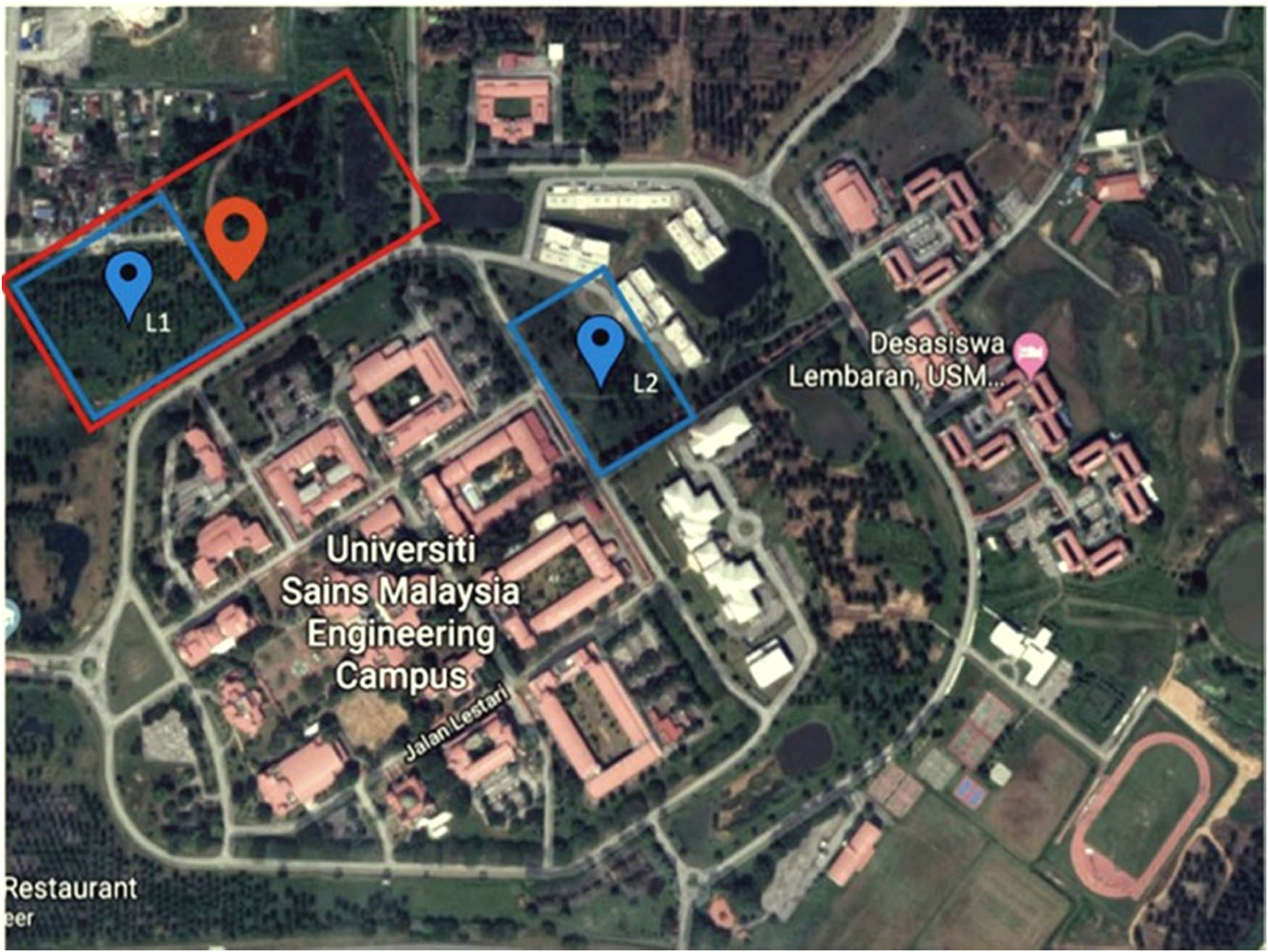
Locations, where the information is collected, are depicted on a map. The blue boxes designated the first location (L1) and the second location (L2) depicts the test flight sites, while the red box denotes the data reception region.
Video resolution is reduced to 426 × 240. Annotating objects beforehand can help save resources during preparation. The set of data is manually labeled using MATLAB Labeler of video. Every video frame has a rectangle Region of Interest (RoI) drawn around all of the tree trunks due to the in-built algorithm. The rectangular RoI surrounding the tree trunk is shown in Figure 3.
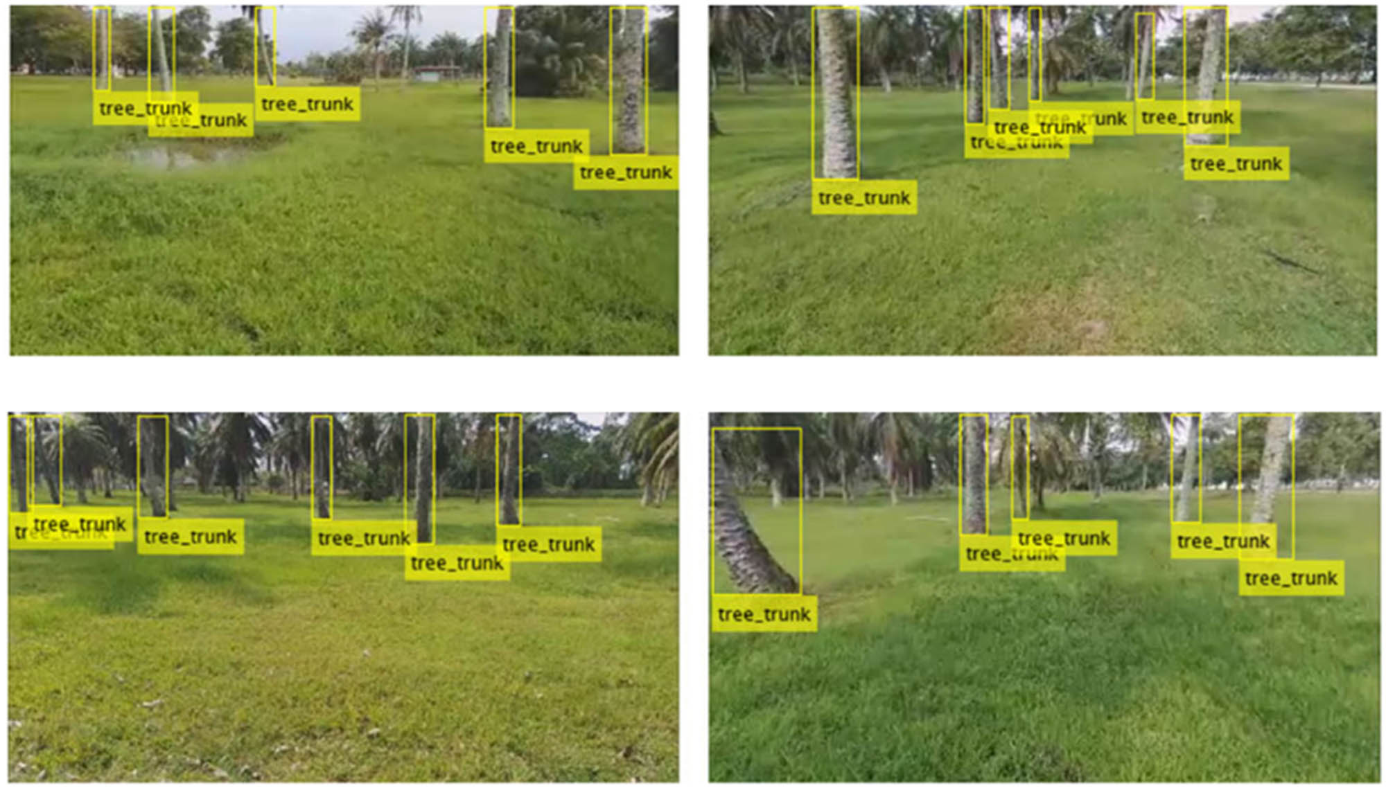
Truth examples with labels. Images of tree trunks are enclosed in bounding boxes with labels.
Consequences for society at large arise from precision forestry’s use of CNN-based algorithms. For starters, it facilitates precise species identification and categorization of trees, which aids in the creation of effective management plans for forests. Second, it helps with pest and disease control in forests by making it easier to spot and monitor problems. Last but not least, it provides more accurate inventory estimations, which help optimize resource allocation and improve forest sustainability. Finally, the automation and scalability of precision forestry operations are enhanced when CNN-based algorithms are combined with remote sensing technologies. Algorithms based on CNNs are essential to the development of precision forestry and the advancement of sustainable forest management.
3.2 Avoidance motion
3.2.1 Obstacles detection and localization
Detection is cast-off to regulate the mobility of an autonomously navigating UAV. By feeding each raw picture into its input layer, the trained model can identify obstructions. The detection model computes bounding boxes for obstacles relative to the image’s top left corner as the origin. The coordinate (x i , y i ) picture system is depicted in Figure 4. The minimum and maximum x and y coordinates of the enclosing box are (x i1,min, y i1,max), separately. Our obstacle-evading system’s recognition model can identify tree trunks in images. In the final images, the trunks of trees with reliability ratings above 0.7 are displayed. Most low-confidence bounding boxes are either incorrect results or thin, small tree trunks that indicate faraway objects. There is no impact on UAV navigation from these findings. This decreases the size of avoidance bounding boxes where confidence is low, saving computational resources.

The axis of the photograph corresponds to the width and height of a box that can contain an obstruction.
3.2.2 Dangerous obstacles identification
After collecting the directs of the obstacles, it is necessary to recognize the obstacles that the UAV would encounter. They are “major roadblocks” to this research. The method interprets the altitudes of leaping boxes as cues for deepness. The controller tells the UAV to keep moving ahead at a constant pace until it encounters an obstacle. Critical obstacles are either directly in the path of the UAV’s flight or contained behind a protective barrier.
As can be seen in Figure 5, the buffer zone around the UAV camera is fixed at a distance of 0.5 m. It prevents the UAV from colliding with obstacles in its path. It describes the dimensions of the UAVs and suggests some secure locations for flight. The method must also allow the UAV to detect objects at a distance of at least 1 m. Some potential travel inconveniences, such as the time it takes for image data as well as motion control commands to be relayed via Wi-Fi, can be mitigated using this precautionary approach. As was said before, the dimensions of the boxes that define the boundaries of an image are used to determine the depth. This value is variable depending on the UAV’s altitude. In theory, the UAV’s altitude might be adjusted based on feedback from sonar measurements, but in practice, the UAV rarely maintains a constant altitude. Reasons for this include the unsteadiness of measures and UAVs in the face of things like side winds and gusts, as well as soft, uneven ground.

The zenith reference axis of the UAV from above. The unlit region denotes the 0.5 m radius of the UAV’s safe operating area. The horizontal viewing angle of the onboard camera is 80°. When the location is 1 m forward of the camera, the calculated distance of the actual straight interpretation is 1.678 m.
To achieve this, the “height ratio” (or “h ratio”) parameter is set. It is the proportion of an image’s height to the highest point of a barrier in the image. It can determine whether or not an object is hazardous at a specified height. Therefore, the altitude ratio of the item at various flying a height, Z, in meters, may be calculated using Eq. (1):
where VFOV (vertical field of view) is measured in degrees, h img (image height) is measured in pixels, and f (camera focal length) is measured in pixels.
Figure 4 illustrates how to use the bounding box’s y i1,max value to test whether or not Condition 1 is met. Whenever the proportion of y i1,max to h img is higher or equal to h ratio, as shown in Eq. (2), Condition 2 is satisfied. The item is approaching the UAV, as indicated by this.
Keep in mind that the height of the obstruction in the picture is not used, but rather y i1,max is used. This is due to the fact that, starting at y i = 0, at the highest point of the image, the boxes that define the boundaries may not entirely enclose the obstruction. The leaves of a tree, for instance, can completely conceal the summit of the tree.
To verify Hypothesis 2, we look to the x-value of the visual frame to locate the obstacles. The x i1 dimensions of the boxes that surround an object are utilized to determine if an object’s location is within the UAV’s safe zone, as shown in Figure 4. Since the mistake was corrected via the calibration of the camera and the ROS framework, it was assumed in this study that the onboard camera was a pinhole camera. So, the limit of the barrier’s xi1 coordinates within the safety limit can be described as:
where x i1,min, x i1,max, and x i1,c are smallest, highest, and midpoint x-coordinate of the leaping box, correspondingly. To calculate wobj’s size if its location is 1 m from the camera, Eq. (4) is used.
where HFOV is the straight field of vision of the camera (in angles) and wimg is the distance of the image (in pixels). The two variables in Eqs. (2) and (3) are used to zero down on the most pressing issues.
3.2.3 Estimated reference for the desired heading
After sensing a major obstruction, the UAV is turned in the direction of flight. The desired direction reference also takes into account the nearing but not yet essential obstructions. In this work, we call this type of barrier a “warning obstacle.” These obstacles have bounding boxes that are taller than one-third of the image. The UAV’s path can be made less bumpy by factoring these obstacles into the revised bearing angle. This makes for a more relaxed navigational experience than methods that merely look for and avoid the most dangerous hazards. In agricultural tree plantations, CNN-based algorithms may be useful for UAV image processing and navigation. The first potential use for UAVs is in crop monitoring and harvest forecasting by analysis of high-resolution aerial photographs. Second, these algorithms might help locate and map weeds, which would allow for more effective pesticide application. Third, they might help in the detection of agricultural pests and illnesses, which would enable preventative measures to be taken and substantial damage to crops to be kept to a minimum. Finally, algorithms based on CNNs might optimize water use in agriculture by providing precision irrigation by evaluating vegetation indices and soil moisture patterns. These use cases demonstrate the potential for CNN-based algorithms to significantly impact industries such as precision agriculture. To find the necessary heading reference, the largest clear area is found along the image’s x-axis. An illustration of the preferred bearing reference is shown in Figure 6; the bounding boxes represent the detected obstructions. Distances on the horizontal axis between significant and warning obstacle bounding boxes, as well as between obstacle-bounding boxes and image borders, are represented by the symbol w i . The number of blank pixels along the x-axis is denoted by the subscript i. According to Figure 6’s green vertical line, the area with the highest w i value also has the fewest obstructions. The necessary direction reference can be obtained by finding the exact center of the largest region free of obstacles. The available area is too limited for the UAV to pass through if the highest possible amount of w i is below eighty pixels, which is equivalent to a range of 0.32 m while the UAV is one meter ahead. The best possible value for x under these conditions.

The green vertical line on the camera displays the desired heading. Image borders (w 1) and identified obstacles (w 4) are at w 1 and w 4 horizontal distances, respectively, while warning and significant obstacles (w 2 and w 3) are at w 2 and w 3 vertical distances.
W img is the picture border. This prevents the UAV from continuing toward an area where it would be unsafe to fly. Once x has been determined, the steering angle can be determined using Eq. (5). Positive values of the steering angle indicate a clockwise rotation, while negative values indicate a counterclockwise one. Using the addition in Eq. (6), we can determine the correct heading reference. The UAV halt and steering angle approach is described in detail in approach 1.
3.2.4 The UAV’s motion control
In this research, the flight controller is modified to use a simple method of motion control to verify the proposed strategy. The UAV will continue ahead at a steady speed from its initial place until it is stopped by the detection model. The UAV’s height is kept at a steady 1.5 m by using input from sonar measurements. When a major obstruction is detected, the UAV is given instructions to rotate to the specified bearing. This rotation is regulated by the subsequent equation for the UAV’s velocity of rotation about the zb axis:
where K p is calculated to be 0.5 in order to quickly reach the target heading angle. Figure 5 illustrates that the zb plane is downward-pointing and transverse to the xbyb plane. First, a UAV must be built.
| Algorithm 1 UAV steering decision framework. | ||
|---|---|---|
| Require: Raw Image received from the UAV | ||
| Ensure: Corresponding steering angle | ||
| 1: Resize the image into 426 × 240 pixels | ||
| 2: Detect the presence of tree trunks in the images | ||
| 3: Output the bounding boxes coordinates (x i j.min , y i j.min , x i j.max , y i j.max ) | ||
| 4: Determine the centroid coordinates for each bounding box | ||
| 5: for Each obstacle detected do | ||
| 6: | if An obstacle is a critical obstacle then | |
| 7: | Command the UAV to stop and hover at the same position | |
| 8: | Determine the largest obstacle-free space | |
| 9: | Calculate the corresponding steering angle | |
| 10: | end if | |
| 11: end for | ||
In agricultural tree plantations, CNN-based algorithms may be useful for UAV image processing and navigation. The first potential use for UAVs is in crop monitoring and harvest forecasting by analysis of high-resolution aerial photographs. Second, these algorithms might help locate and map weeds, which would allow for more effective pesticide application. Third, they might help in the detection of agricultural pests and illnesses, which would enable preventative measures to be taken and substantial damage to crops to be kept to a minimum. Finally, algorithms based on CNNs might optimize water use in agriculture by providing precision irrigation by evaluating vegetation indices and soil moisture patterns. These examples demonstrate how CNN-based algorithms might revolutionize precision agriculture in a variety of fields.
The current scenario is examined to make sure that is no major impediment in the way. Note that certain safeguards are taken for the sake of safety during actual tests. To prevent the projected image transmission delay from impacting the flight, the UAV is instructed to advance at a constant, slow pace of 0.1 m/s. Additionally, the unmanned aircraft first pauses and then turns according to the intended heading reference when a crucial impediment is detected. Its purpose is to make sure the current incident’s image is used as part of the navigational compass reading. In this study, we suggest an obstacle avoidance approach and undertake experiments to test its viability. The flight efficiency can be further enhanced in future applications by making use of more sophisticated platform results.
4 Results
The performance of CNN-based navigation algorithms may be enhanced in challenging tree-planting conditions in a variety of ways. The first is that multi-modal sensor fusion, like LiDAR or depth sensors, might enhance obstacle detection by providing extra depth information. Second, by pre-training the CNN on large data sets that contain a variety of environmental circumstances transfer learning may improve its resilience and flexibility. Finally, including spatial transformers or attention algorithms in the CNN design may help reduce the effect of occlusions. In tree-planting situations, the network’s generalization and variance tolerance might be improved with the use of data augmentation approaches.
4.1 Optical detection result
4.1.1 The performance of the various scratch models
The paper describes the training using four scratched models as detectors, each with slightly different requirements, in Section 3.1.1. This is done to learn how many convolutional layers a detection model needs and how many total training photos affect its accuracy. Sixty photos that were not included in the training of each detector were used to assess its performance. Figure 7 displays the precision-recall curves for each detector to help evaluate their overall performance. Detector A outperforms the other detectors when thinking of the median precision value. Detector A has the highest possible recall value of all detectors at 0.76. In other words, the detection success rate for the crucial impediments in the photos was higher when using Detector A because it correctly identified a higher percentage of true trunks of trees in the test images.

Test results with precision-recall curves. (a) Detector A, (b) detector B, (c) detector C, and (d) detector D.
There are several advantages to using CNN-based algorithms for forest inventory and monitoring. To start, they offer efficient and automated analysis of large-scale aerial photographs, which allows quick and accurate evaluations of forest inventories. Second, these algorithms may facilitate timely intervention and conservation measures by helping to find and monitor forest concerns like deforestation or illicit logging. One disadvantage is that it requires a lot of computational power and training data that is labeled. Findings may not be transferable to other types of forests due to errors in classification or detection. Using CNN-based algorithms may greatly improve the monitoring of forests and inventory, but the advantages and cons must be weighed carefully before implementation.
In addition, Detectors B, C, and D were compared to investigate how many convolutional layers have an impact on tree detection. The average precision is highest for Detector B, then Detector D, and finally Detector C. Test findings show that Detector C has the maximum sensitive tree trunk identification presentation, as indicated by its smallest maximal recall. This illustrates that the regular accuracy of the indicator is not enhanced by the addition of convolutional layers. The algorithm with two layers of convolution outperforms other shallow layout models on the tree trunk identification task.
As a result, the following step involves selecting and training the most effective scratch model to serve as the trunk of the tree detector. To improve the detection performance of the model with two layers of convolution, it is recommended that it be trained on more images.
4.1.2 Models that have already been trained are compared to the scratch model
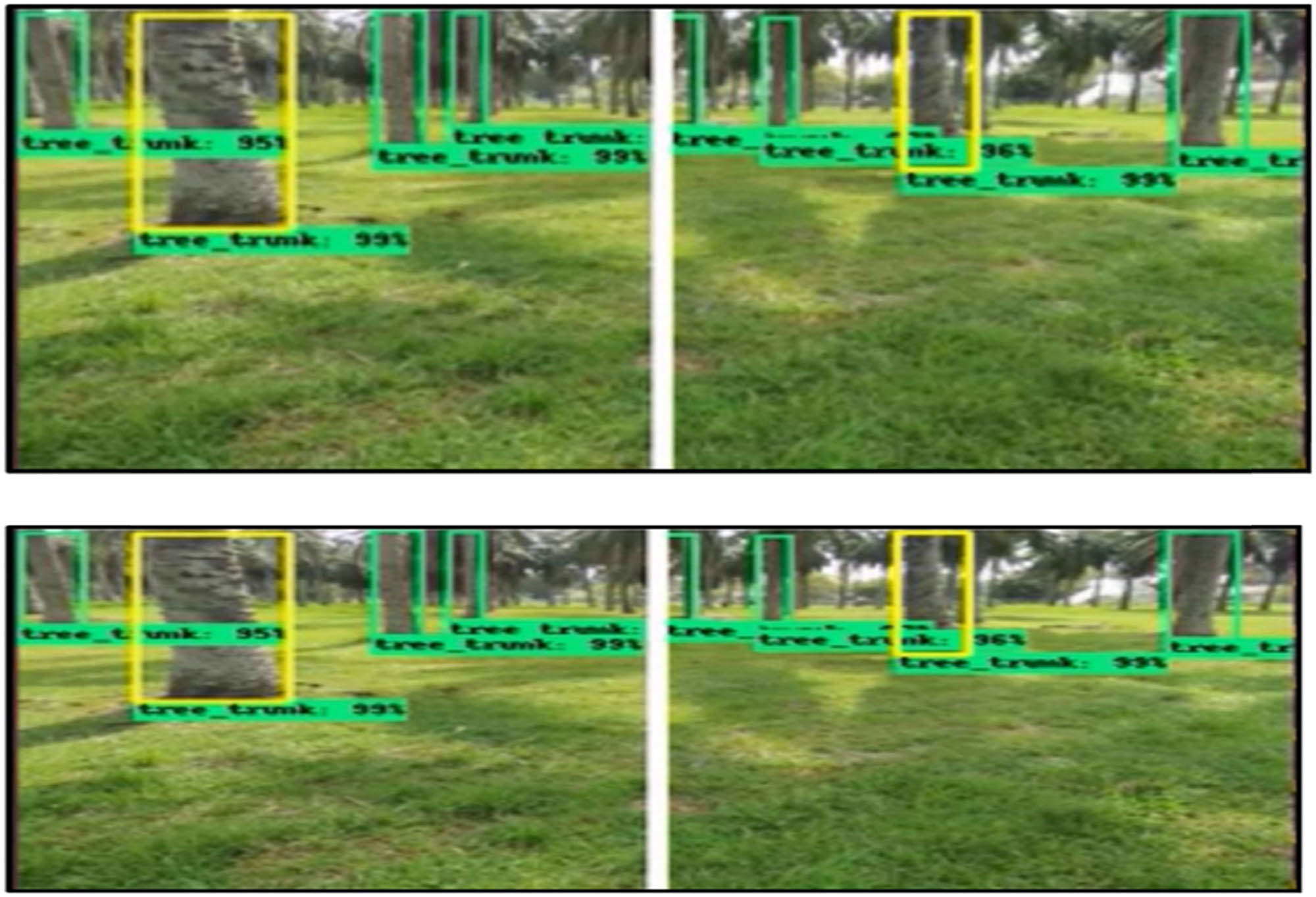
The collection includes photographs taken in a range of lighting conditions. There are 4,689 photos taken from a 12-minute flying movie that make up the training data set. There are an overall of 23860.0 tree trunk explanations in these pictures. After the models were trained, they were confirmed using a couple-minute flying movie made up of 514 still photographs taken in the same location. Test image detection results are shown randomly in Figure 8. The output photos in Figure 1 show both of the pre-trained models can reliably identify tree trunks in a wide range of lighting and shadow circumstances. Figure 8 shows test photos where most output boxes cover full tree trunks. Furthermore, there are no blatant false positives generated by any of these two pre-trained models. This graphical representation shows that the results are non-linear.
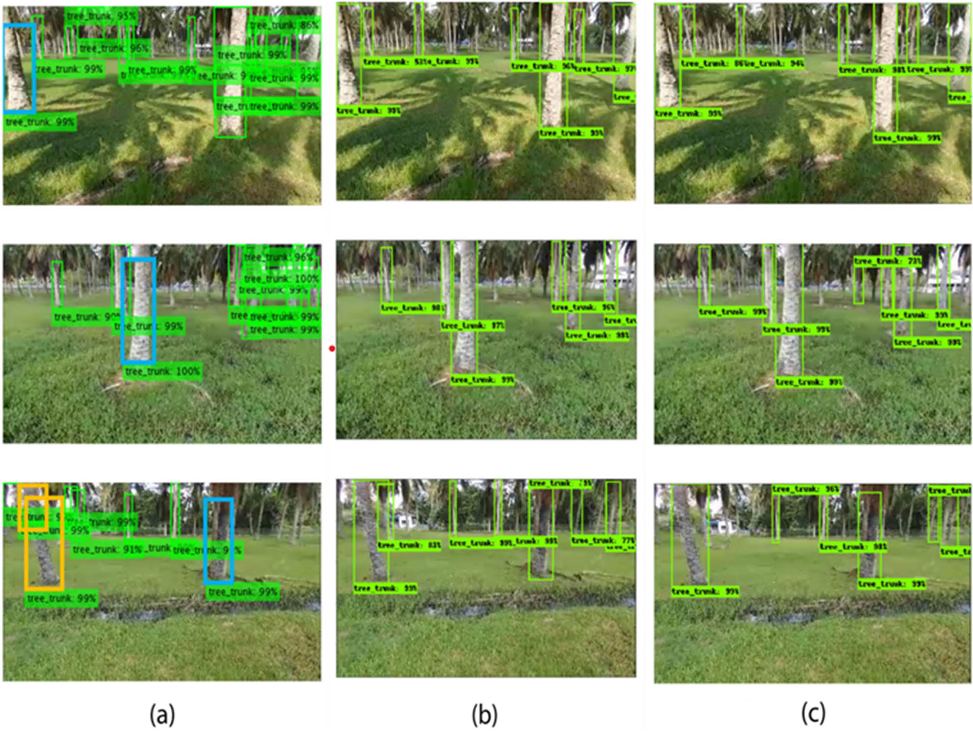
Some illustrations of test consequences for detecting tree trunks. (a) Scratch model, (b) Resnet-50, and (c) Inception V2.
However, test images created using the scratch model consistently feature false positive squares with high confidence values bordering the image’s backdrop. In Figure 8’s blue boxes, we can see that many of the scratch algorithm’s boundaries did not cover the complete length of a tree trunk. Additionally, two distinct orange bounding boxes encompassed the bulk of the large obstacles in the photographs. The height of the barrier is used as an extent indicator in the UAV’s obstacle avoidance method; therefore, accurate bounding is essential. Incomplete or inconsistent box coverage prevents the strategy from labeling an oncoming obstacle as essential. In this way, the UAV will run into the obstacle and crash. This scratch model may not be feasible to use in the suggested approach due to the high quality of its output. Figure 9 depicts the accuracy-recall graphs of both the scratch version and the pre-trained models. With respect to maximal recall, both pre-trained models fared better than the scratch model. That is to say, the pre-trained models can reliably foretell boundaries around trunks of trees and will not miss oncoming obstructions. Table 3 displays the regular accuracy and swiftness of detection for both the scratch model and the previously trained models. We can use the middle Images.
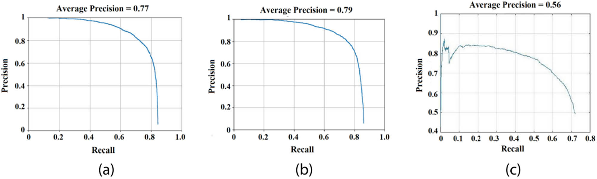
Compare untrained and trained models using the precision-recall curve. (a) Resnet-50, (b) Inception V2, and (c) scratch model.
Parameter variations among four trained detectors
| Parameter | Pre-trained models | Scratch model | |
|---|---|---|---|
| Resnet-50 | Inception V2 | ||
| Average precision | 0.77 | 0.79 | 0.56 |
| Detection speed per frame (s) | 2.02 | 0.36 | 1.3 |
Outputs are depicted as green squares with labeled categories and self-assurance scores. The orange boxes characterize the two obstacles that have been identified by the model, while the blue packets represent partial leaping boxes.
Many variables influence the precision and dependability of CNN-based navigation algorithms used in tree plantations. Having sufficient and high-quality training data is essential. It is possible that the effectiveness of the algorithm might be enhanced by amassing test datasets that include a broad variety of trees, lighting situations, and occlusions. Constructing the network’s architecture and fine-tuning the hyper-parameters is the second step. It is possible to improve navigation accuracy by adjusting CNN architecture and hyper-parameters like learning rate and batch size. Algorithms’ dependability may be enhanced by the application of techniques like data enhancement, mechanisms of attention, and transfer learning to deal with problems like strong extraction of features and occlusion management.
With the same technology, Inception v2 has a detection speed that is 9.5 times that of Resnet-50 because to its expansive architecture.
Using CNN-based algorithms for UAV image processing and navigation has many drawbacks in forested environments. First, a lack of data may limit algorithms’ generalizability to diverse kinds of trees and planting situations. To fully train the methods and get around this restriction, it is necessary to have access to larger and more varied datasets. Second, it may be challenging to accurately recognize items and move through them due to occlusion and complicated tree topologies. Modern design concepts like attention systems and spatial transformers might offer answers to these issues. Third, computational power and processing time might be reduced limitations, but these can be addressed by using effective hardware or by enhancing network architecture. Finally, there may be barriers to understanding CNN-based algorithms, necessitating extra methods for detailing the process of making decisions to guarantee transparency and credibility.
The more rapid R-CNN plus Inception v2 is used as the indicator in our obstacle-avoiding organization since it reliably and quickly generates detection boxes. In addition, this method generates bounding boxes that include the complete extent of obstacles, including important barriers in the flight path of the UAV.
4.2 Result of obstacle avoidance
4.2.1 Flight test setup
We enjoy the ahead camera for its use in obstacle avoidance. Test flights yield 60 fps stills. Sonar always travels at a height of 1.5 m. During flights, the Bebop 2’s GPS coordinates and attitude angles are recorded for verification later on.
The Bebop 2 Software Development Kit (SDK) 2 talks to the ROS Airborne autonomous driver1. Both 2.4 and 5 GHz Wi-Fi can be used for UAV communication.
This ROS Kinetic setup is running on Ubuntu 16.04. The Core Intel core i5-7500U MB the central processing unit (32GB RAM, and Nvidia 940MX in the ground control station are needed for the difficult mathematical computations required by the detecting system.
The locations of the two test areas are depicted in Figure 2. In the first place, there’s the actual area from where the training information was drawn. If the initial test in Location 1 goes well, the identical UAV will try flying over another forest. The preceding action
Use a variety of datasets to see how well your system can handle obstacles. The corridors and buildings in the training photos are replaced with an unfamiliar landscape. Both regions feature dense forest cover, making it safe for the UAV to navigate overhead.
4.2.2 Results of detection during flight test
Each bounding box’s height-to-width ratio indicates the significance of the obstacles encountered thus far. The flying tests display three colors: green, yellow, and red.
Whether the items were too close to the UAV or too far away, or whether they were approaching it. For instance, far-away obstacles are indicated by green bounding boxes. Non-linear relation can be seen in Figure 14. The UAV’s proximity to trees triggers the display of yellow boundary boxes when it is beyond the 1 m protective zone. These obstacles are known as “warning barriers.”
Putting up warning barriers alerts the UAV that there is a potential hazard in the area. When deciding what to do next when a crucial barrier has been located, the algorithm takes this into account. However, the UAV is not instructed to land or adjust its trajectory.
If there are not any significant problems, as directed by the white line in the middle of the image, the heading will remain. As can be seen in Figure 10, this indicates that it is okay for the UAV to proceed.

Conditions suitable for UAV travel. Since it is okay for the UAV to keep moving forward, the optimal heading is represented by the white line, which remains central in the image.
When the primary barrier is located, a red box is positioned around it. The system then recalculates its course to take use of the available space. Figure 11 demonstrates how the target direction can be located in every scene where the red and yellow rectangles coexist. The white line has moved, demonstrating that the system has identified the most significant barrier and selected an alternate route to traverse it. This strategy not only steers the UAV far from a particularly dangerous obstruction but also towards the path with the least amount of obstacles directly ahead.

Examples of the detection of critical obstacles. There is a white line in the picture that points in the direction the UAV is supposed to go.
Using CNN-based algorithms for UAV image processing and navigation provides substantial difficulties in forested areas. First, a lack of relevant data may restrict algorithms’ application to a wide variety of tree species and growth situations. More varied data are required to fully train the methods and remove this restriction. Second, accurate detection and navigation may be challenging because of occlusion and complex tree topologies. Newer design concepts, such as attention systems and the spatial transformer, may provide answers to these problems. Third, as technology and network architecture advance, there may be less limits on computer power and processing speed. If CNN-based algorithms grow too complex for the average person to understand, we may need to find other means of communicating the decision-making process to maintain transparency and credibility.
4.2.3 Avoidance control for flight evaluations
Using GPS information from 11 separate trials, the flight paths of the UAVs used in these tests are shown on a map in Figure 12. Experiment distances are also shown here for your perusal.
Each trial’s worth of GPS data from the UAV’s navigational tests.
In every test, the UAV successfully avoided any potentially fatal frontal obstacles. Despite the detector’s lack of familiarity with Location 2, the UAV successfully navigated around any significant impediments. Because of the system’s durability, it can be applied to autonomous UAV guidance in additional oil palm regions with varying topography and climate. All flight trials were successfully completed by the UAV until the operator physically shut down the program. In order to analyze UAV mobility throughout trials, its heading and pitch angles, as shown in Figure 13, were recorded. This graph’s quick pitch angle peaks indicate that the UAV was brought to a halt. When UAVs stop moving, they tilt up. The images are shown in Figure 13. After the unexpected highs, the UAV was sent in a different direction to pass by the critical obstruction. The system of detection can identify major obstructions and calculate alternatively desired headings even while operating in extreme darkness. The UAV completed the 113-m flight on its own in the experiment after a five-minute period and 46 s to complete. With five different maneuvers, the UAV was able to escape collisions. After each discontinuation, the system went in the path with the fewest obstacles. Because of this improvement, UAVs no longer have to come to a complete stop before steering. The initial detection result is shown in Figure 14. The UAV flew right past two cautionary yellow boxes. The required bearing reference stayed rather close to the middle, allowing forward progress. The UAV was programmed to fly ahead under its own power. A major roadblock is depicted at 50.5 s in Figure 15. In order to face the largest available area free of obstacles, the algorithm halted the UAV and spun it 7° counterclockwise. At 84.9 and 128 s, when the crucial obstacle was found, the UAV paused and rotated. The inclination of the wheel was established by the available clearance. At 276.66 s, the UAV went at a significantly lesser altitude than it had been maintaining with sonar measurement feedback. The sensor’s height reading was skewed upwards because of the soft soil. The UAV was lowered by the controller. Figure 16 depicts the results of an analysis of methods used to detect and avoid obstacles. The UAV’s altitude made the tree’s trunk look abnormally little. When the UAV approached the tree trunk, it immediately stopped. The UAV came to a halt 0.7 m from the danger zone’s edge. Figure 16 shows that the UAV had to make two course corrections because of its restricted field of view and the presence of obstacles. Even after its initial rotation of −19°, the blockage remained the primary factor in its inability to move forward. The UAV performed admirably by traveling an additional –13°. The obstacle was located far from the UAV’s intended path after the second yaw. Therefore, the UAV kept moving forward.

What follows from the initial realization? The white stripe in the middle of the photo indicates the desired direction, allowing the UAV to go in that direction. Nearby barriers that aren’t crucial enough to halt the UAV are depicted as yellow boxes. (a) Location 1 and (b) Location 2.

In one of the attempts, the red and blue arcs represent the field and caption of the UAV, respectively. The images that triggered the system’s halt are also included. Important roadblocks are depicted with red rectangles in the images.

The top images display the detection outcome, while the bottom images depict the UAV from the viewpoint of the observer prior to and following the time the UAV rotated after the system perceived a crucial obstacle about 50.40 s. (a) Before steering and (b) after steering.

Below are photographs of the UAV from the point of view of an observer before controlling their vehicles, after the first control, and after the subsequent steering; above are images of the detection outcome after the UAV motionless at 276.66 s. There is no critical roadblock in image c. This means the image will focus on the chosen heading. (a) Before steering, (b) after the first steering and (c) after the second steering.
5 Conclusion
An original method for UAV autonomy in a forest was proposed in this study. Previously, detecting blockages required using sensors situated outside the system; our solution eliminates the requirement for such sensors. The algorithm predicts the placement of obstacles on an individual basis after obtaining the frontal images using the onboard camera. When an obstruction is detected in a photograph, the model notifies the computer controlling the UAV of its precise location.
UAV algorithms that employ convolution neural networks (CNNs) for analyzing pictures and moving through forests provide new research opportunities. We can improve algorithms for 3D mapping, species categorization, and forest assessment of health by first investigating how multipurpose sensor data, such as Laser or hyperspectral images, may be comprised in them. Second, in order to better handle temporal dependencies and optimize navigation and tracking, we look at the use of recurring or attention-based CNN designs in dynamic plantation environments. Third, AI methods are elucidated so that experts may have trust in and respect the algorithm’s decision-making. These developments might be put into practice to improve inventory estimation, tree health monitoring, and resource allocation for responsible forest management.
The UAV, which stands for an UAV, was able to successfully recognize all of the trunks of trees that were harmful to its guidance and successfully execute the tree-avoiding maneuver on its own, despite the fact that the flying altitude was not kept constant during the 11 tests.
-
Funding information: There is no funding.
-
Author contributions: The author has accepted responsibility for the entire content of this manuscript and approved its submission.
-
Conflict of interest: There is no conflict of interest.
References
[1] Lee HY, Ho HW, Zhou Y. Deep learning-based monocular obstacle avoidance for unmanned aerial vehicle navigation in tree plantations. J Intell Robot Syst. 2020 Dec 8;101(1):5.10.1007/s10846-020-01284-zSearch in Google Scholar
[2] Ammar A, Koubaa A, Benjdira B. Deep-learning-based automated palm tree counting and geolocation in large farms from aerial geotagged images. Agronomy. 2021 Aug;11(8):1458.10.3390/agronomy11081458Search in Google Scholar
[3] Windrim L, Bryson M, McLean M, Randle J, Stone C. Automated mapping of woody debris over harvested forest plantations using UAVs, high-resolution imagery, and machine learning. Remote Sens. 2019 Jan;11(6):733.10.3390/rs11060733Search in Google Scholar
[4] Barbosa BDS, Ferraz GA, Costa L, Ampatzidis Y, Vijayakumar V, dos Santos LM. UAV-based coffee yield prediction utilizing feature selection and deep learning. Smart Agric Technol. 2021 Dec 1;1:100010.10.1016/j.atech.2021.100010Search in Google Scholar
[5] Selvaraj MG, Valderrama M, Guzman D, Valencia M, Ruiz H, Acharjee A. Machine learning for high-throughput field phenotyping and image processing provides insight into the association of above and below-ground traits in cassava (Manihot esculenta Crantz). Plant Methods. 2020 Jun 14;16(1):87.10.1186/s13007-020-00625-1Search in Google Scholar PubMed PubMed Central
[6] Sandino J, Pegg G, Gonzalez F, Smith G. Aerial mapping of forests affected by pathogens using UAVs, hyperspectral sensors, and artificial intelligence. Sensors. 2018 Apr;18(4):944.10.3390/s18040944Search in Google Scholar PubMed PubMed Central
[7] Islam N, Rashid MM, Wibowo S, Xu CY, Morshed A, Wasimi SA, et al. Early weed detection using image processing and machine learning techniques in an Australian chilli farm. Agriculture. 2021 May;11(5):387.10.3390/agriculture11050387Search in Google Scholar
[8] Fichtel L, Frühwald AM, Hösch L, Schreibmann V, Bachmeir C, Bohlander F. Tree localization and monitoring on autonomous drones employing deep learning. 2021 29th Conference of Open Innovations Association (FRUCT); 2021 May 12–14; Tempere, Finland. IEEE, 2021. p. 132–40.10.23919/FRUCT52173.2021.9435549Search in Google Scholar
[9] Badrloo S, Varshosaz M, Pirasteh S, Li J. Image-based obstacle detection methods for the safe navigation of unmanned vehicles: A review. Remote Sens. 2022 Jan;14(15):3824.10.3390/rs14153824Search in Google Scholar
[10] Santos L, Santos FN, Filipe V, Shinde P. Vineyard segmentation from satellite imagery using machine learning. In: Moura Oliveira P, Novais P, Reis LP, editors. Progress in artificial intelligence. Cham, Switzerland: Springer International Publishing; 2019. p. 109–20. (Lecture Notes in Computer Science)10.1007/978-3-030-30241-2_10Search in Google Scholar
[11] Hao Z, Lin L, Post CJ, Mikhailova EA, Li M, Chen Y, et al. Automated tree-crown and height detection in a young forest plantation using mask region-based convolutional neural network (Mask R-CNN). ISPRS J Photogramm Remote Sens. 2021 Aug 1;178:112–23.10.1016/j.isprsjprs.2021.06.003Search in Google Scholar
[12] Torres VAMF, Jaimes BRA, Ribeiro ES, Braga MT, Shiguemori EH, Velho HFC, et al. Combined weightless neural network FPGA architecture for deforestation surveillance and visual navigation of UAVs. Eng Appl Artif Intell. 2020 Jan 1;87:103227.10.1016/j.engappai.2019.08.021Search in Google Scholar
[13] Narmilan A, Gonzalez F, Salgadoe ASA, Powell K. Detection of white leaf disease in sugarcane using machine learning techniques over UAV multispectral images. Drones. 2022 Sep;6(9):230.10.3390/drones6090230Search in Google Scholar
[14] Bhattacharyay D, Maitra S, Pine S, Shankar T, Mohiuddin G. Future of Precision Agriculture in India. In: Maitra S, Gaikwad DJ, Shankar D., editors. Protected Cultivation and Smart Agriculture. New Delhi, India: New Delhi Publishers; 2020. p. 289–99.10.30954/NDP-PCSA.2020.32Search in Google Scholar
[15] Kadethankar A, Sinha N, Burman A, Hegde V. Deep learning based detection of rhinoceros beetle infestation in coconut trees using drone imagery. In: Singh SK, Roy P, Raman B, Nagabhushan P, editors. Computer Vision and Image Processing. Singapore: Springer; 2021. p. 463–74. (Communications in Computer and Information Science)10.1007/978-981-16-1086-8_41Search in Google Scholar
[16] Apolo-Apolo OE, Pérez-Ruiz M, Martínez-Guanter J, Valente J. A cloud-based environment for generating yield estimation maps from apple orchards using UAV imagery and a deep learning technique. Front Plant Sci. 2020;11:1086. [cited 2023 May 16]. https://www.frontiersin.org/articles/10.3389/fpls.2020.01086.10.3389/fpls.2020.01086Search in Google Scholar PubMed PubMed Central
[17] Kefauver SC, Buchaillot ML, Segarra J, Fernandez Gallego JA, Araus JL, Llosa X, et al. Quantification of Pinus pinea L. Pinecone productivity using machine learning of UAV and field images. Env Sci Proc. 2022;13(1):24.10.3390/IECF2021-10789Search in Google Scholar
[18] Kulbacki M, Segen J, Knieć W, Klempous R, Kluwak K, Nikodem J, et al. Survey of drones for agriculture automation from planting to harvest. 2018 IEEE 22nd International Conference on Intelligent Engineering Systems (INES); 2018 Jun 21–23; Las Palmas de Gran Canaria, Spain. IEEE, 2018. p. 000353–8.10.1109/INES.2018.8523943Search in Google Scholar
[19] Darwin B, Dharmaraj P, Prince S, Popescu DE, Hemanth DJ. Recognition of bloom/yield in crop images using deep learning models for smart agriculture: A review. Agronomy. 2021 Apr;11(4):646.10.3390/agronomy11040646Search in Google Scholar
[20] Oh S, Chang A, Ashapure A, Jung J, Dube N, Maeda M, et al. Plant counting of cotton from UAS imagery using deep learning-based object detection framework. Remote Sens. 2020 Jan;12(18):2981.10.3390/rs12182981Search in Google Scholar
[21] Yu K, Hao Z, Post CJ, Mikhailova EA, Lin L, Zhao G, et al. Comparison of classical methods and mask R-CNN for automatic tree detection and mapping using UAV imagery. Remote Sens. 2022 Jan;14(2):295.10.3390/rs14020295Search in Google Scholar
[22] Mumuni F, Mumuni A, Amuzuvi CK. Deep learning of monocular depth, optical flow and ego-motion with geometric guidance for UAV navigation in dynamic environments. Mach Learn Appl. 2022 Dec 15;10:100416.10.1016/j.mlwa.2022.100416Search in Google Scholar
[23] Li L, Mu X, Chianucci F, Qi J, Jiang J, Zhou J, et al. Ultrahigh-resolution boreal forest canopy mapping: Combining UAV imagery and photogrammetric point clouds in a deep-learning-based approach. Int J Appl Earth Obs Geoinf. 2022 Mar 1;107:102686.10.1016/j.jag.2022.102686Search in Google Scholar
[24] Deng X, Tong Z, Lan Y, Huang Z. Detection and Location of Dead Trees with Pine Wilt Disease Based on Deep Learning and UAV Remote Sensing. AgriEngineering. 2020 Jun;2(2):294–307.10.3390/agriengineering2020019Search in Google Scholar
[25] Yang Q, Shi L, Han J, Yu J, Huang K. A near real-time deep learning approach for detecting rice phenology based on UAV images. Agric For Meteorol. 2020 Jun 15;287:107938.10.1016/j.agrformet.2020.107938Search in Google Scholar
[26] Meivel S, Maheswari S. Remote sensing analysis of agricultural drone. J Indian Soc Remote Sens. 2021 Mar 1;49(3):689–701.10.1007/s12524-020-01244-ySearch in Google Scholar
[27] Chew R, Rineer J, Beach R, O’Neil M, Ujeneza N, Lapidus D, et al. Deep neural networks and transfer learning for food crop identification in UAV images. Drones. 2020 Mar;4(1):7.10.3390/drones4010007Search in Google Scholar
[28] Maimaitijiang M, Sagan V, Sidike P, Hartling S, Esposito F, Fritschi FB. Soybean yield prediction from UAV using multimodal data fusion and deep learning. Remote Sens Env. 2020 Feb 1;237:111599.10.1016/j.rse.2019.111599Search in Google Scholar
© 2023 the author(s), published by De Gruyter
This work is licensed under the Creative Commons Attribution 4.0 International License.
Articles in the same Issue
- Research Articles
- The regularization of spectral methods for hyperbolic Volterra integrodifferential equations with fractional power elliptic operator
- Analytical and numerical study for the generalized q-deformed sinh-Gordon equation
- Dynamics and attitude control of space-based synthetic aperture radar
- A new optimal multistep optimal homotopy asymptotic method to solve nonlinear system of two biological species
- Dynamical aspects of transient electro-osmotic flow of Burgers' fluid with zeta potential in cylindrical tube
- Self-optimization examination system based on improved particle swarm optimization
- Overlapping grid SQLM for third-grade modified nanofluid flow deformed by porous stretchable/shrinkable Riga plate
- Research on indoor localization algorithm based on time unsynchronization
- Performance evaluation and optimization of fixture adapter for oil drilling top drives
- Nonlinear adaptive sliding mode control with application to quadcopters
- Numerical simulation of Burgers’ equations via quartic HB-spline DQM
- Bond performance between recycled concrete and steel bar after high temperature
- Deformable Laplace transform and its applications
- A comparative study for the numerical approximation of 1D and 2D hyperbolic telegraph equations with UAT and UAH tension B-spline DQM
- Numerical approximations of CNLS equations via UAH tension B-spline DQM
- Nonlinear numerical simulation of bond performance between recycled concrete and corroded steel bars
- An iterative approach using Sawi transform for fractional telegraph equation in diversified dimensions
- Investigation of magnetized convection for second-grade nanofluids via Prabhakar differentiation
- Influence of the blade size on the dynamic characteristic damage identification of wind turbine blades
- Cilia and electroosmosis induced double diffusive transport of hybrid nanofluids through microchannel and entropy analysis
- Semi-analytical approximation of time-fractional telegraph equation via natural transform in Caputo derivative
- Analytical solutions of fractional couple stress fluid flow for an engineering problem
- Simulations of fractional time-derivative against proportional time-delay for solving and investigating the generalized perturbed-KdV equation
- Pricing weather derivatives in an uncertain environment
- Variational principles for a double Rayleigh beam system undergoing vibrations and connected by a nonlinear Winkler–Pasternak elastic layer
- Novel soliton structures of truncated M-fractional (4+1)-dim Fokas wave model
- Safety decision analysis of collapse accident based on “accident tree–analytic hierarchy process”
- Derivation of septic B-spline function in n-dimensional to solve n-dimensional partial differential equations
- Development of a gray box system identification model to estimate the parameters affecting traffic accidents
- Homotopy analysis method for discrete quasi-reversibility mollification method of nonhomogeneous backward heat conduction problem
- New kink-periodic and convex–concave-periodic solutions to the modified regularized long wave equation by means of modified rational trigonometric–hyperbolic functions
- Explicit Chebyshev Petrov–Galerkin scheme for time-fractional fourth-order uniform Euler–Bernoulli pinned–pinned beam equation
- NASA DART mission: A preliminary mathematical dynamical model and its nonlinear circuit emulation
- Nonlinear dynamic responses of ballasted railway tracks using concrete sleepers incorporated with reinforced fibres and pre-treated crumb rubber
- Two-component excitation governance of giant wave clusters with the partially nonlocal nonlinearity
- Bifurcation analysis and control of the valve-controlled hydraulic cylinder system
- Engineering fault intelligent monitoring system based on Internet of Things and GIS
- Traveling wave solutions of the generalized scale-invariant analog of the KdV equation by tanh–coth method
- Electric vehicle wireless charging system for the foreign object detection with the inducted coil with magnetic field variation
- Dynamical structures of wave front to the fractional generalized equal width-Burgers model via two analytic schemes: Effects of parameters and fractionality
- Theoretical and numerical analysis of nonlinear Boussinesq equation under fractal fractional derivative
- Research on the artificial control method of the gas nuclei spectrum in the small-scale experimental pool under atmospheric pressure
- Mathematical analysis of the transmission dynamics of viral infection with effective control policies via fractional derivative
- On duality principles and related convex dual formulations suitable for local and global non-convex variational optimization
- Study on the breaking characteristics of glass-like brittle materials
- The construction and development of economic education model in universities based on the spatial Durbin model
- Homoclinic breather, periodic wave, lump solution, and M-shaped rational solutions for cold bosonic atoms in a zig-zag optical lattice
- Fractional insights into Zika virus transmission: Exploring preventive measures from a dynamical perspective
- Rapid Communication
- Influence of joint flexibility on buckling analysis of free–free beams
- Special Issue: Recent trends and emergence of technology in nonlinear engineering and its applications - Part II
- Research on optimization of crane fault predictive control system based on data mining
- Nonlinear computer image scene and target information extraction based on big data technology
- Nonlinear analysis and processing of software development data under Internet of things monitoring system
- Nonlinear remote monitoring system of manipulator based on network communication technology
- Nonlinear bridge deflection monitoring and prediction system based on network communication
- Cross-modal multi-label image classification modeling and recognition based on nonlinear
- Application of nonlinear clustering optimization algorithm in web data mining of cloud computing
- Optimization of information acquisition security of broadband carrier communication based on linear equation
- A review of tiger conservation studies using nonlinear trajectory: A telemetry data approach
- Multiwireless sensors for electrical measurement based on nonlinear improved data fusion algorithm
- Realization of optimization design of electromechanical integration PLC program system based on 3D model
- Research on nonlinear tracking and evaluation of sports 3D vision action
- Analysis of bridge vibration response for identification of bridge damage using BP neural network
- Numerical analysis of vibration response of elastic tube bundle of heat exchanger based on fluid structure coupling analysis
- Establishment of nonlinear network security situational awareness model based on random forest under the background of big data
- Research and implementation of non-linear management and monitoring system for classified information network
- Study of time-fractional delayed differential equations via new integral transform-based variation iteration technique
- Exhaustive study on post effect processing of 3D image based on nonlinear digital watermarking algorithm
- A versatile dynamic noise control framework based on computer simulation and modeling
- A novel hybrid ensemble convolutional neural network for face recognition by optimizing hyperparameters
- Numerical analysis of uneven settlement of highway subgrade based on nonlinear algorithm
- Experimental design and data analysis and optimization of mechanical condition diagnosis for transformer sets
- Special Issue: Reliable and Robust Fuzzy Logic Control System for Industry 4.0
- Framework for identifying network attacks through packet inspection using machine learning
- Convolutional neural network for UAV image processing and navigation in tree plantations based on deep learning
- Analysis of multimedia technology and mobile learning in English teaching in colleges and universities
- A deep learning-based mathematical modeling strategy for classifying musical genres in musical industry
- An effective framework to improve the managerial activities in global software development
- Simulation of three-dimensional temperature field in high-frequency welding based on nonlinear finite element method
- Multi-objective optimization model of transmission error of nonlinear dynamic load of double helical gears
- Fault diagnosis of electrical equipment based on virtual simulation technology
- Application of fractional-order nonlinear equations in coordinated control of multi-agent systems
- Research on railroad locomotive driving safety assistance technology based on electromechanical coupling analysis
- Risk assessment of computer network information using a proposed approach: Fuzzy hierarchical reasoning model based on scientific inversion parallel programming
- Special Issue: Dynamic Engineering and Control Methods for the Nonlinear Systems - Part I
- The application of iterative hard threshold algorithm based on nonlinear optimal compression sensing and electronic information technology in the field of automatic control
- Equilibrium stability of dynamic duopoly Cournot game under heterogeneous strategies, asymmetric information, and one-way R&D spillovers
- Mathematical prediction model construction of network packet loss rate and nonlinear mapping user experience under the Internet of Things
- Target recognition and detection system based on sensor and nonlinear machine vision fusion
- Risk analysis of bridge ship collision based on AIS data model and nonlinear finite element
- Video face target detection and tracking algorithm based on nonlinear sequence Monte Carlo filtering technique
- Adaptive fuzzy extended state observer for a class of nonlinear systems with output constraint