Equilibrium stability of dynamic duopoly Cournot game under heterogeneous strategies, asymmetric information, and one-way R&D spillovers
-
Jianjun Long


Abstract
Bounded rationality, asymmetric information, and R&D spillovers are widely existed in monopoly markets, and they have been researched separately by a large number of literatures; however, there are few works that discussed both R&D spillovers and asymmetric information in oligopolistic games with bounded rational firms. Considering that R&D spillovers only flow from the R&D leader to the R&D follower, a duopoly Cournot game with heterogeneous expectations and asymmetric information is presented. In our model, a firm with private information of his marginal cost is designed, and the coefficient of R&D spillovers is introduced. Interesting findings show the following: (i) In a static duopoly Cournot game with perfect rationality, the equilibrium output of firm 1 with private information is negatively related to R&D spillovers and the probability of high marginal cost, while firm 2’s equilibrium output is positively correlated with them. (ii) In a dynamic duopoly Cournot game with asymmetric information and heterogeneous expectations, if firms adopt adaptive expectation and naïve expectation respectively, the Nash equilibrium is always globally asymptotically stable; if they use adaptive expectation and gradient dynamical expectation respectively, the Nash equilibrium tends to be locally asymptotically stable under certain conditions. Furthermore, the bigger the probability of high marginal cost or R&D spillovers are, the more volatile the monopoly market is, while higher technology innovation efficiency (TIE) of firm 1 is conducive to the stability of the product market. Our study would have theoretical and practical significance to the technological innovation activities of homogeneous products in oligopoly markets.
1 Introduction
Oligopoly means that a tiny number of firms produce the same or similar products and supply the whole market, and it attracts attentions of mathematicians, economists, and management scientists for its complexity, diversity, and social authenticity. One of the classic oligopoly games is the Cournot model, which was pioneered by Augustin Cournot in 1838 [1]. In this typical model, two sellers compete simultaneously with no collusion in a product market and they determine the optimal outputs based on each other’s actions.
The classical Cournot game requires participants to have all the information and to be completely rational, but this strong assumption often contradicts the reality. Due to the complexity and uncertainty of economic environment, as well as the limitation of computing power and cognition ability, incomplete information is ubiquitous in market economy. Asymmetric information is a special case of incomplete information, it mainly comes from the asymmetry of information held by market participants due to the imperfection of the market itself, the difference of information acquisition ability between buyers and sellers, and the difference of industry information caused by the division of labor. Participants with access to more valid information tend to be in a good position to trade in the market. The widespread existence of information asymmetry in economic society has attracted the attention of a large number of scholars, and relevant papers mainly focus on cost information asymmetry [2,3] and demand information asymmetry [4,5]; there are also some studies on information asymmetry from the perspectives of innovation efficiency asymmetry [6] and productivity asymmetry [7].
Traditional economics has always been premised on complete rationality, that is, the actor has access to all information, and so he can choose the one that maximizes the utility among various schemes. However, decision-makers are bounded rational in reality, and they are influenced by many factors such as physiology, motivation, and ability. First, it is almost impossible to make the optimal decision completely rational in a short time in the face of many changing factors. Second, decision-makers also have limited access to information, knowledge, and abilities, and also their abilities to process information are different. Third, decision-makers will also be affected by emotion, value bias, and other irrational factors, and cannot be completely objective and rational when making decisions. Therefore, complete rationality has been criticized for its overstepping reality [8]; bounded rationality, which is closer to reality, has attracted more and more attention; and expectation rules with bounded rationality is more and more valued and applied in modeling monopoly games. As far as we know, naïve [9–11] expectation, adaptive expectation [3,12,13], gradient dynamical expectation [14,15], local monopolistic approximation [16–18], and expectation are the most commonly used decision criteria in extant references.
Research and development (R&D) refers to the systematic activities with clear objectives carried out continuously by research institutions and enterprises. R&D is mainly aimed at acquiring new scientific and technological knowledge and be used to improve technologies, products, and services. It generally refers to product R&D and technological R&D. As an innovation activity, R&D is a crucial source of competitive advantage and an important guarantee of sustainable development of enterprises. As mentioned in many works [19–24], spillovers inevitably occurs in R&D activities. Because of its positive externality, R&D spillovers can reduce the product costs of R&D enterprises, but it can also reduce the enthusiasm of enterprises engaged in R&D activities for malicious free-riding behavior. Besides, due to the differences in R&D capabilities, one-way R&D spillovers is common in reality [19,20], that is, R&D spillovers only flow from R&D leaders to R&D followers. In addition to one-way R&D spillovers, our article also considers another important economic phenomenon: the enterprise cluster, which refers to the geographical aggregation of some closely related enterprises and their supporting institutions in an industry with few leading enterprises as the core [25]. Due to the geographical proximity, organizational proximity, and cognitive proximity, enterprises in the cluster show stronger competitiveness than general enterprises [26] for R&D spillovers. So this article mainly studies the complexity of a duopoly Cournot game with asymmetric information, bounded rationality, and one-way R&D spillovers.
Incomplete information, bounded rationality and one-way R&D spillovers are widespread in the real economic society, and have been studied a lot in oligopoly games. But as far as we know, there are few works integrating asymmetry information and R&D spillovers into dynamic Cournot models with perfect or imperfect rationality. This gives us the impetus to solve the following problems: (i) Whether Bayesian Nash equilibrium outputs exist in a static duopoly Cournot game with asymmetric information and perfect rationality? If it exists, what is the condition? Furthermore, what are the effects of asymmetric information and R&D spillovers on the equilibrium outputs? (ii) In a dynamic duopoly Cournot game with bounded rationality, what are the effects of asymmetric information and R&D spillovers on the equilibrium outputs? (iii) When duopoly firms adopt different bounded expectations, does Bayesian Nash equilibrium exist in the dynamic system? If so, what are the conditions? To address the aforementioned issues, this article constructs a duopoly Cournot model with asymmetric information, where firm 1’s marginal cost is private and firm 2’s marginal cost is well known. We mainly intend to study influences of R&D spillovers and asymmetric information on Nash equilibrium under perfect and bounded rationality, and provide the region where equilibrium outputs exist.
Our research expands the existing works on complex dynamics of oligopoly Cournot games from the perspective of bounded rationality and asymmetric information. Ever since the Cournot model was proposed in 1838, studies revolving around it continued to spring up, and earlier works focused on perfect rationality and complete information [27,28]. As bounded rationality gets more and more attention, many scholars have analyzed Cournot models with bounded rationality and complete information. Reference [29] analyzed complex dynamics in a triopoly Cournot game with different strategies. Reference [30] discussed an investment process in a Cournot game with heterogenous players. Reference [31] established a duopoly Cournot model with relative profits maximization and investigated the effect of the degree of product differentiation on Nash equilibrium. Reference [24] studied the complexities of product differentiation and R&D spillover in a two-stage duopoly Cournot game. Our article differs from the aforementioned references in two ways. First, as we can see the extant works rarely researched asymmetric information in dynamic Cournot games, by contrast, this article introduces asymmetric information of marginal cost and discusses its effect on the stability of equilibrium outputs. Second, our research extends the application of Cournot competition to the enterprise cluster. Since Rand introduced the chaos theory into oligopoly model as early as 1978 [32], scholars are increasingly concerned about the application of bounded rationality in the economic market and social environment, such as Chinese air-conditioning market [33] and enterprise network [21]. Despite the widespread monopoly phenomenon in enterprises clusters, few literature applied bounded rationality to enterprises clusters, References [3,34] discussed bounded rationality and asymmetric information in an enterprise cluster with duopoly firms, but these two articles, respectively, analyzed Bertrand game and Cournot-Bertrand game, which are fundamentally different from the Cournot game studied in this article.
Our research also extends the application of R&D spillovers to nonlinear discrete systems. R&D spillovers refers to the positive externality brought by the knowledge and technology generated by enterprises’ R&D activities. Other cluster enterprises with close distance and frequent staff turnover receive part or all of the knowledge and technology for free to gain profits, and R&D spillovers inevitably occurs [9]. Many works have studied R&D spillovers under perfect rationality [19,20]. The limitations of information acquisition, cognition, computation and other abilities have attracted more and more scholars to pay attention to R&D spillover under bounded rationality [9,21–24]. Reference [3] analyzed the influence of cluster spillovers on price equilibrium under bounded rationality and asymmetric information and found that when duopoly firms adopt different strategies, high cluster spillovers are conducive to market stability. Reference [34] studied the complexity of cluster spillover effect in Cournot–Bertrand mixed game, and found that the influence of cluster spillover effect on the stability of nonlinear system depends on the substitutability between products. Reference [9] investigated the effects of spillovers on the existence of the Nash equilibrium, and figured out that the cost-reduction effect caused by R&D spillovers affected the stability of output deeply. References [21] and [35] discussed R&D externalities in a two-stage monopoly game along networks. Reference [24] analyzed R&D spillover effect in a Cournot duopoly game with product differentiation. Reference [3] analyzed the influence of cluster spillovers on price equilibrium under bounded rationality and asymmetric information, and found that when duopoly firms adopt different strategies, high cluster spillovers is conducive to market stability. Reference [34] studied the complexity of cluster spillover effect in Cournot-Bertrand mixed game, and found that the influence of cluster spillover effect on the stability of nonlinear system depends on the substitutability between products. Our article differs in the following respects: first, we consider one-way R&D spillovers in the process of R&D activities in Cournot games with bounded rational firms, which is different from the assumption of bilateral spillovers in most previous works [3,34]. Second, most existing references discussed R&D spillovers in oligopoly games with bounded rationality or asymmetric information separately, and this article investigates R&D spillovers in a Cournot game combined with bounded rationality and asymmetric information, different from Bertrand game in ref. [3] and hybrid game in ref. [34]. Third, we extend the application of chaos theory to the firms’ R&D process in an enterprise cluster, which is an important economic phenomenon. Except the analysis of R&D spillovers, like most previous articles, we also study the influence of R&D investments, TIE, and asymmetric information on the dynamic equilibrium outputs with the chaos theory.
Several key findings are obtained. First, the equilibrium output and its stable regions are proposed in the dynamic duopoly Cournot game with perfect rationality and asymmetric information, which implies that, the equilibrium output of firm 1 with private information is negatively correlated with R&D spillovers and the probability of firm 1’s high marginal cost, while the equilibrium output of firm 2 is positively correlated with them. The extant references rarely discussed this issue. Second, the Nash equilibrium output is always globally asymptotically stable in a dynamic duopoly Cournot game with asymmetric information and heterogeneous expectations, where two firms adopt adaptive expectation and gradient dynamical expectation, respectively. This finding is different from our common sense that Bayesian Nash equilibrium exists only if players use same expectations, which is verified and simulated in the main reference [36]. Third, in a dynamic duopoly Cournot game with asymmetric information and heterogeneous expectations, where adaptive expectation and gradient dynamical expectation are used, respectively, the Nash equilibrium output is locally asymptotically stable only when the parameters meet certain conditions. Specially, we find that large probability of high marginal cost and big value of R&D spillovers can yield bifurcation, or even chaos, while high TIE is conducive to the stability of the production market.
The rest of our article is arranged as follows. We introduce asymmetric information and one-way R&D spillovers into a static duopoly Cournot model with perfect rationality in Section 2, and the Bayesian Nash equilibrium output is calculated. Section 3 proposes a dynamic Cournot duopoly model with heterogeneous expectations and asymmetric information through one-way R&D spillovers, and the existence of Bayesian Nash equilibrium and its stability region are discussed. In Section 4, various numerical simulation tools, including 1D and 2D bifurcation diagrams, largest Lyapunov exponents, attraction basin, and sensitive dependence on initial conditions, are presented to verify our theoretical analysis, and the management significance is also given. In Section 5, the state variables feedback and parameter variation method is used to control chaos. Section 6 gives a summary of our research finally.
2 Equilibrium outputs of duopoly firms under perfect rationality and asymmetric information
Bayesian Nash equilibrium is used to describe the static game equilibrium with incomplete information, and its definition [37] is as follows: in a static Bayesian game
It is assumed that two firms, denoted by
We assume the inverse demand function is linear and has the form
In the process of R&D, the cost of an enterprise is not only related to its own R&D investments but also closely related to the R&D spillovers. With the assumption that firms have no fixed costs, we consider that the unit cost of an enterprise has a marginal decreasing relationship with its own investment, which means the cost reduction is
Under all aforementioned assumptions, it is easy to know:
To ensure the validity of subsequent propositions, we propose the following condition, which can be worked out from Eqs. (4) and (6) with backward induction:
To acquire the Bayesian Nash equilibrium, we need to obtain the optimal response functions of the two firms. Firm 1’s best reply function
Then the marginal profit of firm 1 is:
We set
or
The mathematical expectation of the best reply function
After obtaining the optimal response for firm 1’s output, we would calculate the best reply function for firm 2. As firm 2 only knows the probability distribution of firm 1’s marginal cost
The marginal profit of firm 2 is:
We set the first order
where
Bayesian Nash equilibrium can be obtained in two steps, assuming that the duopoly has complete information. Step 1: after calculating the expected output of firm 1 in Eq. (4), firm 2 can determine his optimal quantity through Eq. (6). Step 2: firm 1 would determine his optimal output in Eq. (3) after firm 2 ensures its output in step 1. Then the Bayesian Nash equilibrium can be acquired by combining Eqs. (3), (4), and (6).
Propositions 1 and 2, proved in Appendix A, can be obtained through the aforementioned calculations.
Proposition 1
When parameters meet the condition Eq. (1), the expectation of firm 1’s best reply function is
Proposition 2
When parameters meet the condition Eq. (1), Bayesian Nash equilibrium
In this section, Bayesian Nash equilibrium of a static Cournot model with asymmetric information and complete rationality is proposed and given by Eqs. (7) and (8). Eq. (8) implies that, the bigger
3 Stability of dynamic duopoly Cournot model with heterogeneous expectations and asymmetric information
3.1 Adaptive expectation and naïve expectation adopted under asymmetric information
It is assumed that firm 1 has a high marginal cost with the probability
where
Proposition 3
On the hypothesis that firm 1 uses an adaptive expectation and firm 2 adopts a naive expectation, the Bayesian Nash equilibrium of system (9) is always globally asymptotically stable.
We can see the proof of Proposition 3 in Appendix A. Proposition 3 shows that the Bayesian Nash equilibrium may exist stably even if the bounded rational firms adopt different output adjustment strategies. This is very different from findings in most existing works, which usually point out that equilibrium points is asymptotically stable only in two cases, one is that parameters meet certain conditions and the other is that players use homogeneous expectations.
3.2 Adaptive expectation and gradient dynamical expectation adopted under asymmetric information
In this subsection, we consider that firm 1 still adopts adaptive expectation, firm 2 acts as a gradient dynamical expectation player, so firm 2 decides his output on the basis of marginal profit
where
To study the stability of equilibrium points of system (10), we set
Then system (10) has two equilibrium points:
Next we need to study the local stability of equilibrium points, and to this end, it is necessarily to calculate the Jacobian matrix of system (10) at any point
Plug in the specific value of equilibrium points
Proposition 4
If firm 1 chooses an adaptive expectation and firm 2 uses a gradient dynamical expectation, the boundary equilibrium point
Proof
The Jacobian matrix at
Obviously three eigenvalues are
Proposition 5
If firm 1 chooses an adaptive expectation and firm 2 uses a gradient dynamical expectation, the Nash equilibrium point
The proof of Proposition 5 is in Appendix A, and it gives a stable region
where
Substitute
By combining the stable region
Proposition 6
Consider two firms with heterogenous strategies where firm 1 chooses an adaptive expectation and firm 2 adopts a gradient dynamical expectation, and the stability of Bayesian Nash equilibrium increases as
4 Numerical simulation and management significance
In this section, we carry on some numerical experiments to verify typical features of nonlinear dynamical systems (9) and (10), and put forward the management significance in practice. We use various tools, including 1D and 2D bifurcation diagrams, strange attractors, 1D and 2D largest Lyapunov exponents, basins of attraction, and sensitive dependence on initial conditions, to exhibit the existence of bifurcation and chaos.
Figures 1 and 2 show Bayesian Nash equilibrium of system (9) with respect to
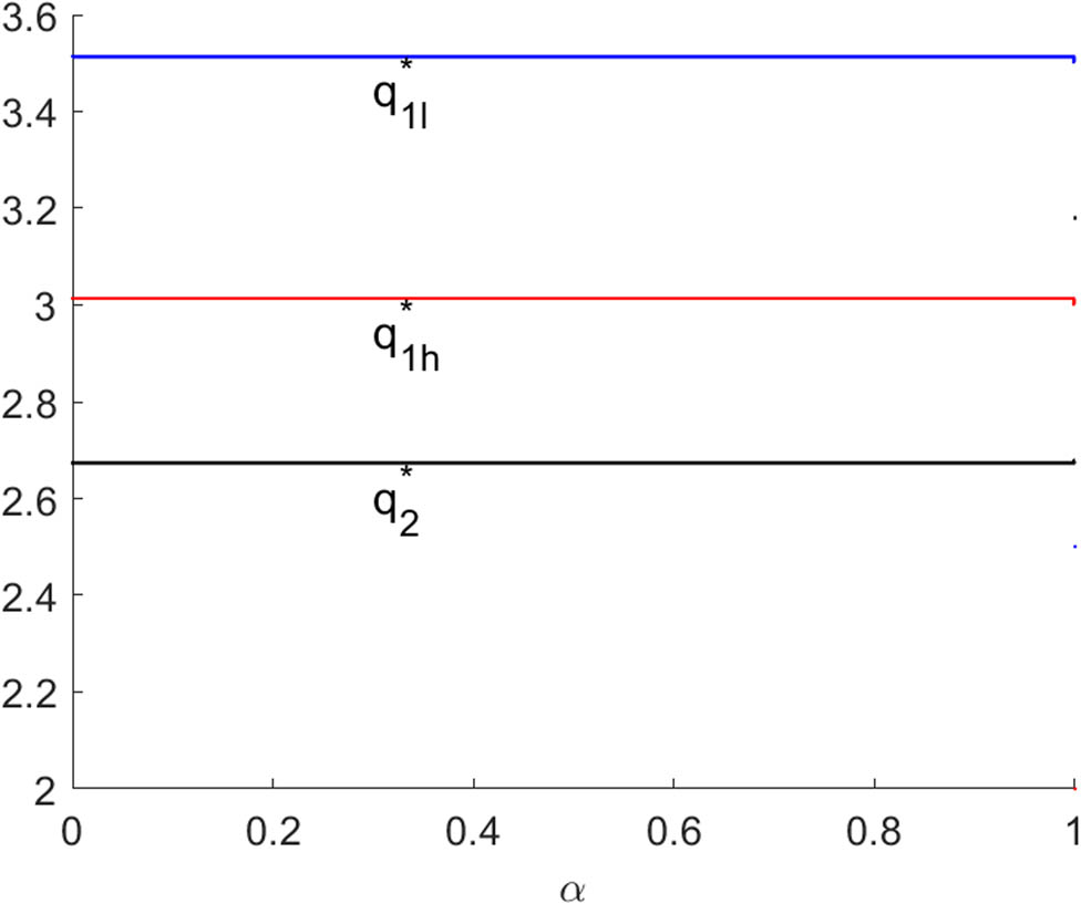
Bayesian Nash equilibrium of system (9) with respect to
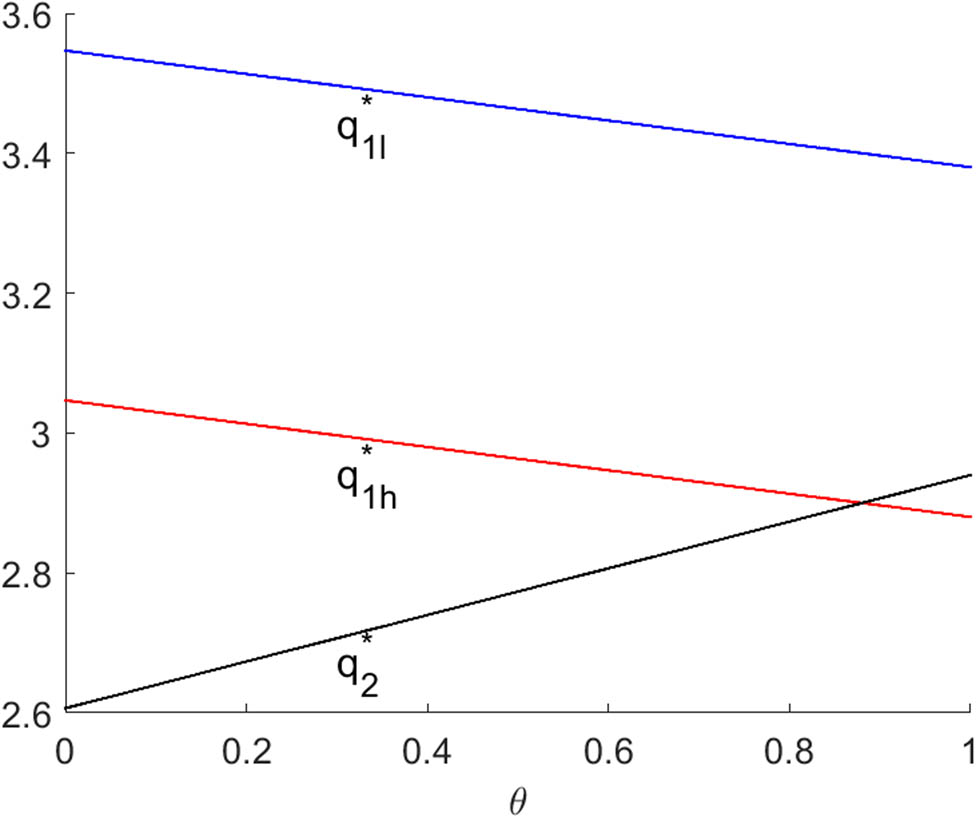
Bayesian Nash equilibrium of system (9) with respect to
Next, we will simulate the trajectory of system (10) under different values of parameters
Figures 3 and 4 present bifurcation diagrams of system (10) with respect to
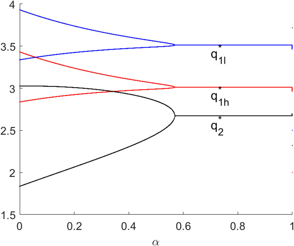
The bifurcaiton diagram of system (10) with respect to
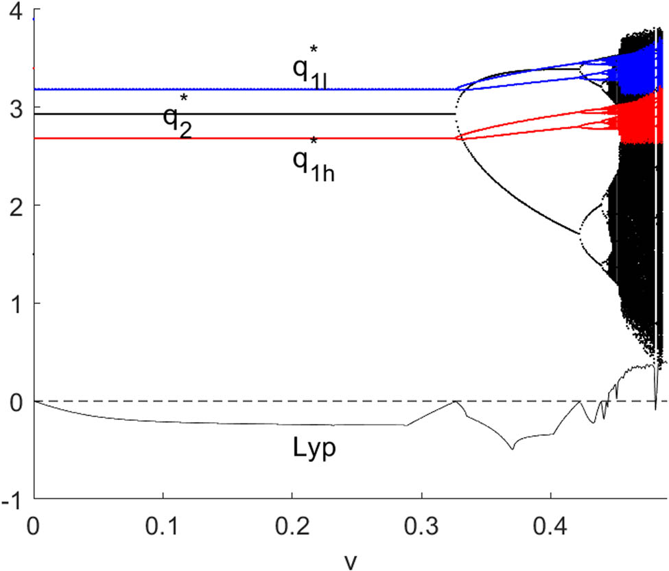
The bifurcaiton diagram of system (10) with respect to
Figures 3 and 4 show the opposite effects of the output adjustment speed on the stability of outputs, and this is mainly because the two firms are in a competitive relationship. Larger
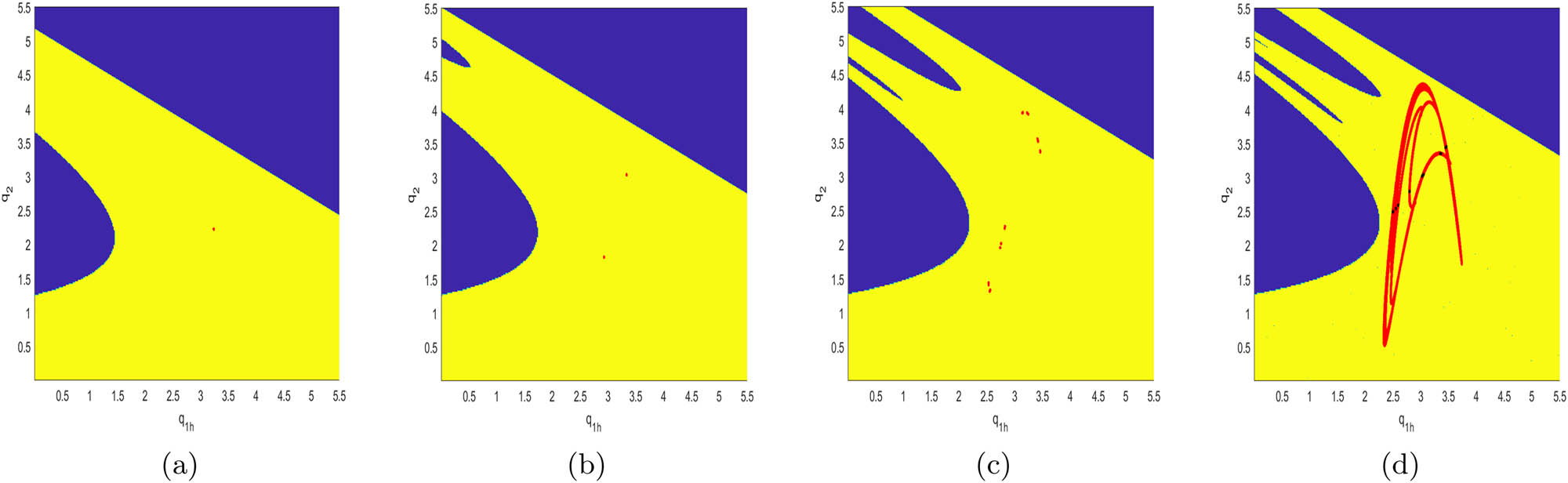
Figure 5(a) shows 2D bifurcation diagram in the
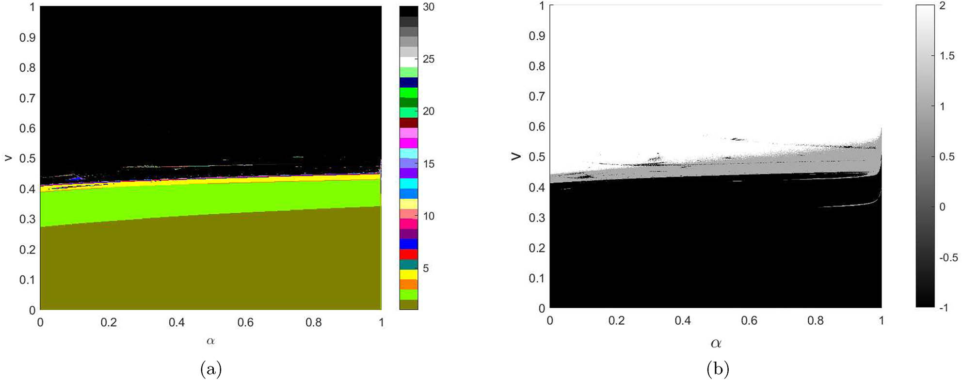
(a) 2D bifurcation diagram in the
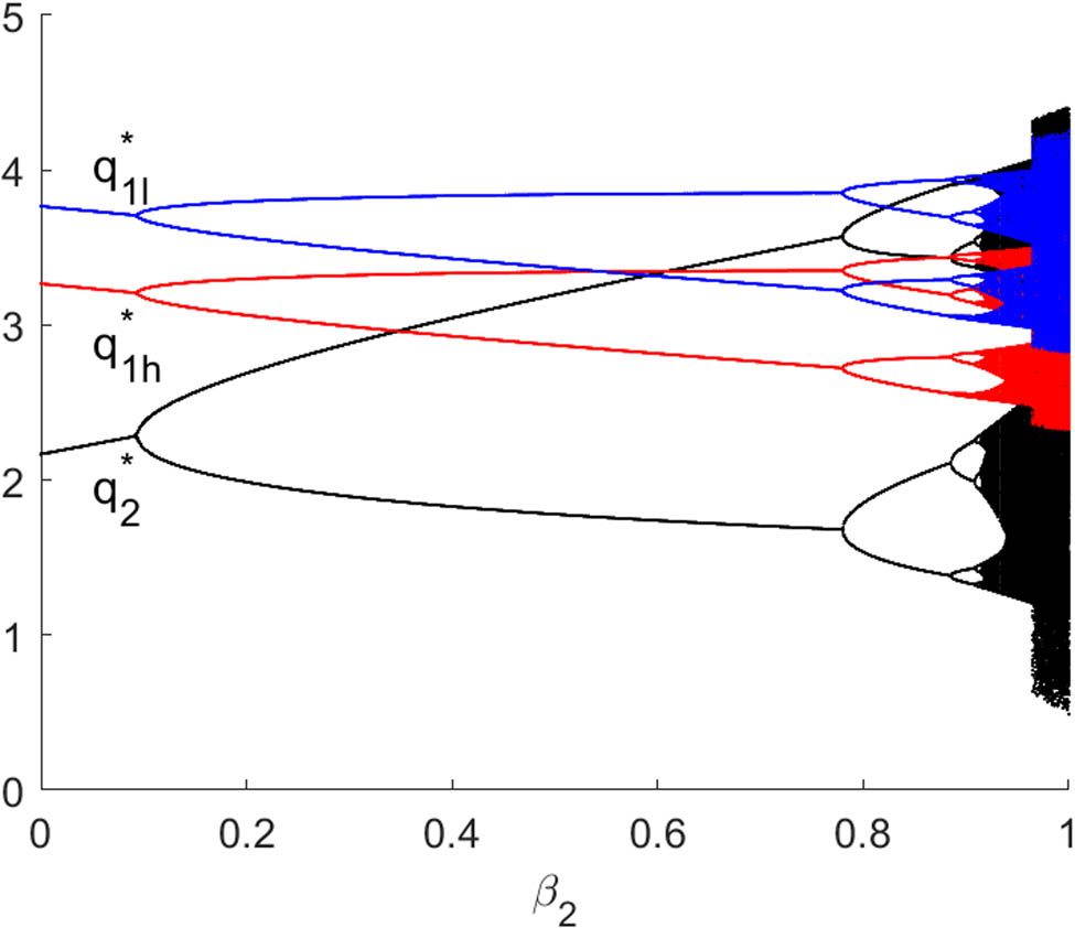
Figures 6 and 7 shows bifurcation diagrams of system (10) with respect to
The bifurcaiton diagram of system (10) with respect to
The bifurcaiton diagram of system (10) with respect to
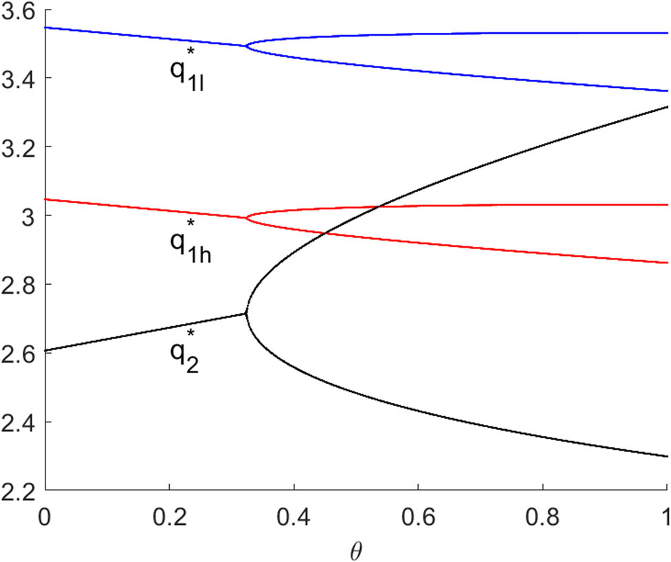
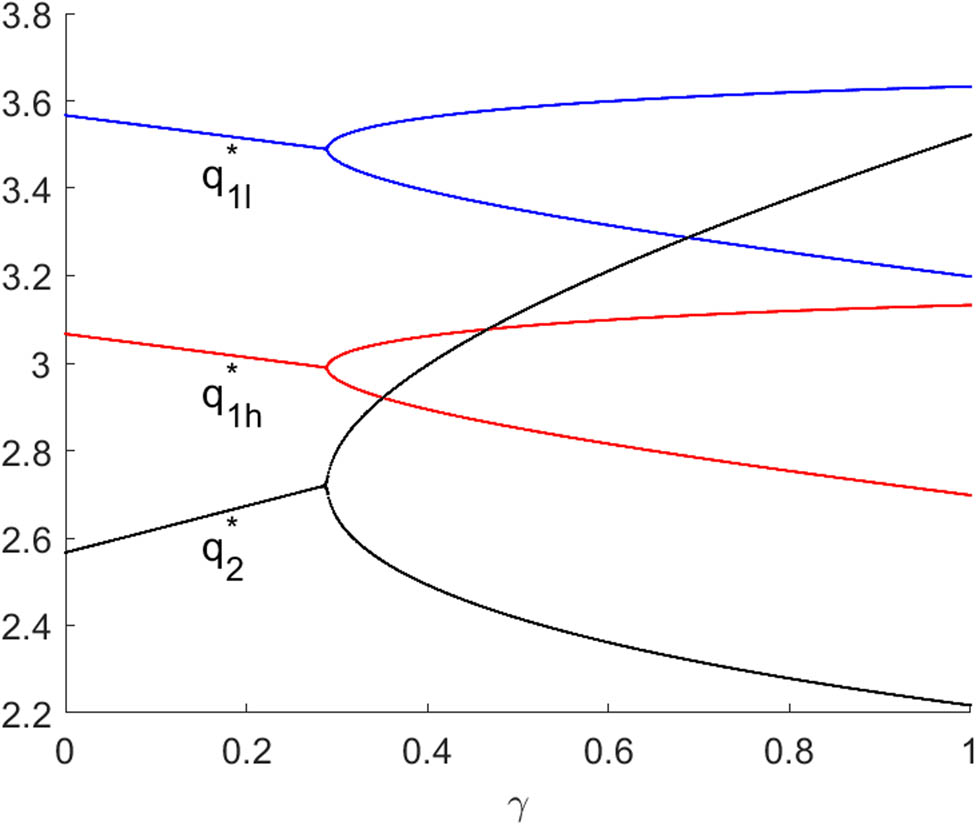
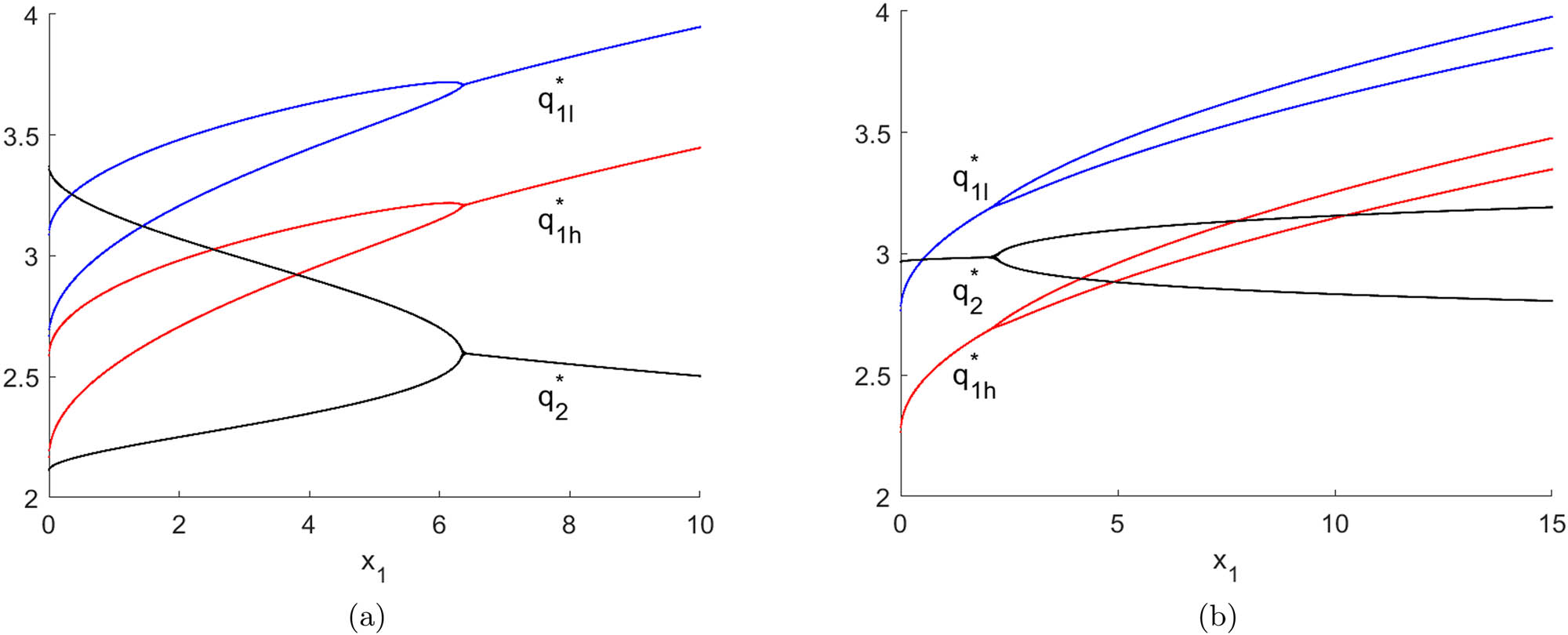
Figures 8 and 9 present bifurcation diagrams of system (10) with respect to
Bayesian Nash equilibrium of system (10) with respect to
Bayesian Nash equilibrium of system (10) with respect to
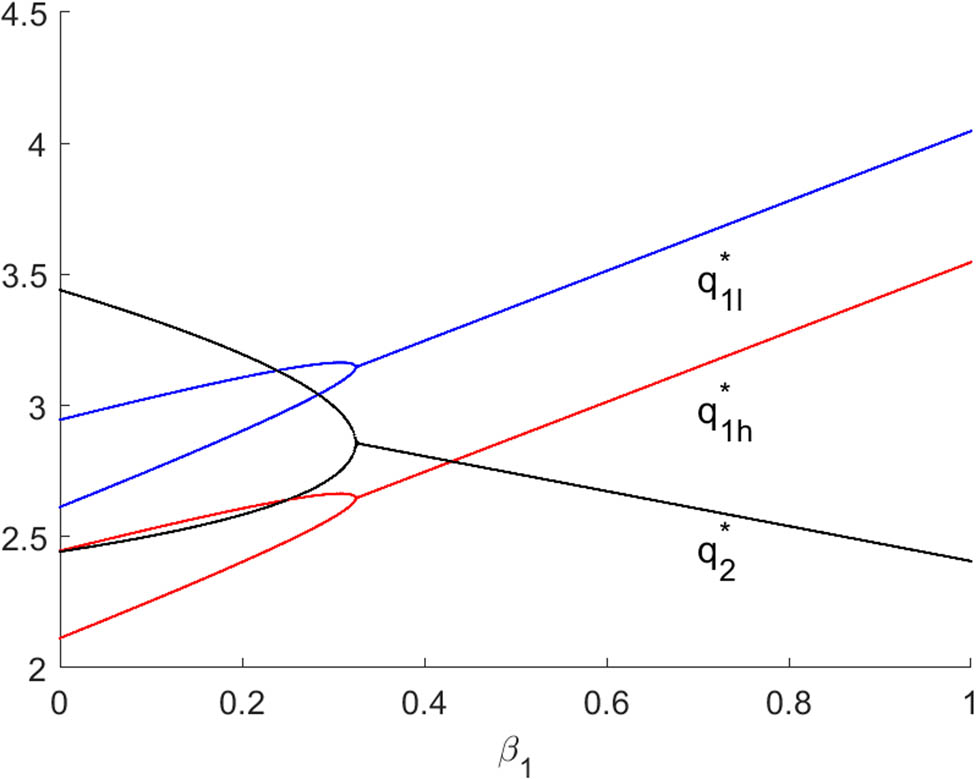
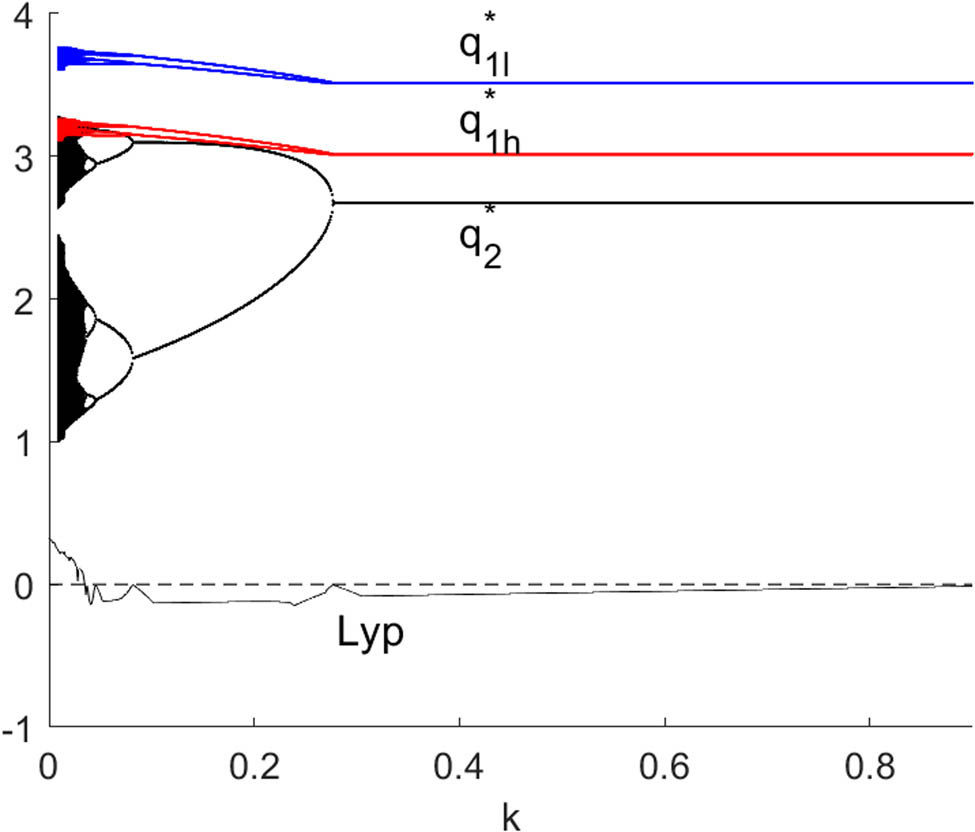
Figures 10 and 11 show the bifurcation diagrams with respect to
The bifurcation diagrams with respect to
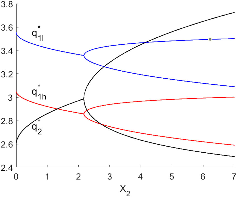
The bifurcaiton diagram of system (10) with respect to
Figures 10 and 11 further validate our theoretical analysis, and the impact of firm 1’s innovation investment on the stability of equilibrium output depends on TIE and R&D spillover between firms. When the firm 1’s TIE is relatively large, the increase of
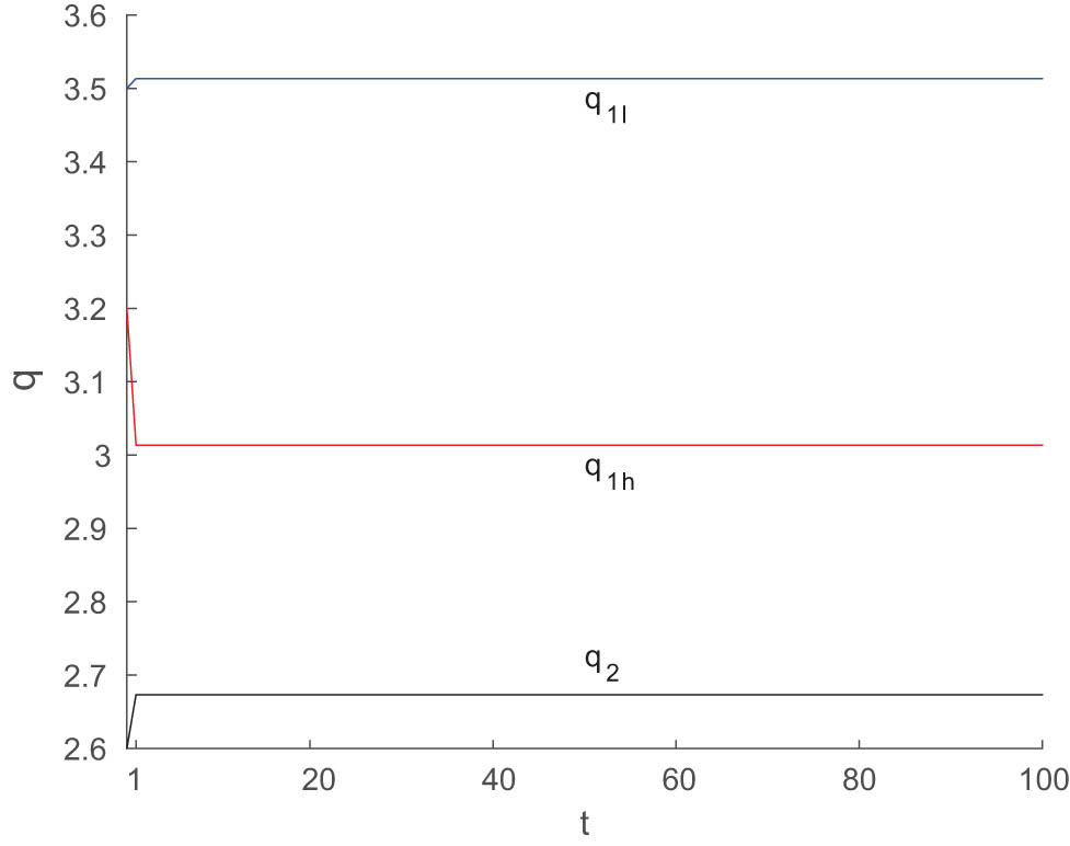
Two important features of chaos are the strange attractor and the sensitivity to initial conditions. Figure 12 shows a chaos attractor at (
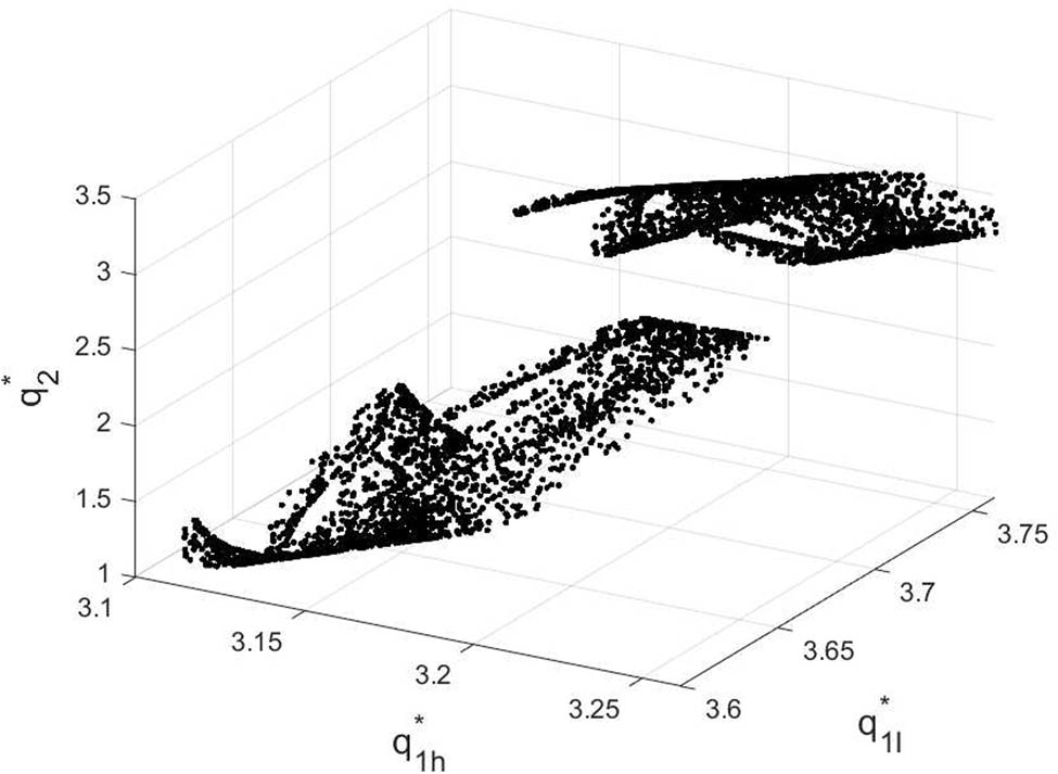
The strange attractor of the system (10) for
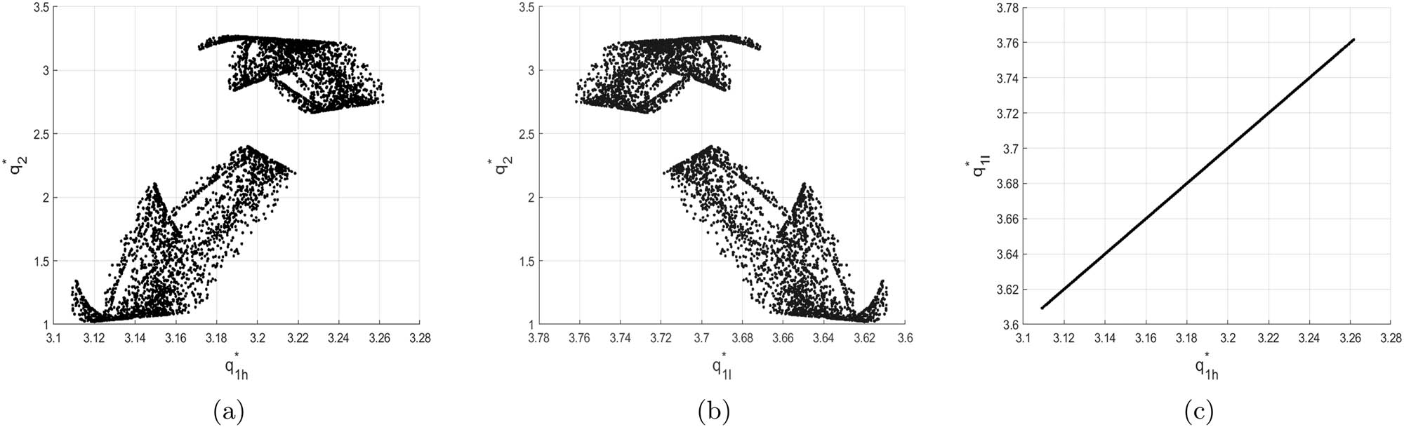
The strange attractor of system (10) in different planes.
![Figure 14
Sensitive dependence of system (10) on initial conditions. The system orbits in the time periods
[
0
,
100
]
\left[0,100]
are plotted with other parameters values
(
a
,
c
,
β
1
,
β
2
,
θ
,
v
)
\left(a,c,{\beta }_{1},{\beta }_{2},\theta ,v)
=
(
10
,
2
,
0.6
,
0.3
,
0.2
,
0.42
)
\left(10,2,0.6,0.3,0.2,0.42)
and
(
q
1
h
(
0
)
,
q
1
l
(
0
)
,
q
2
(
0
)
)
({q}_{1h}\left(0),{q}_{1l}\left(0),{q}_{2}\left(0))
=
(
3.2
,
3.5
,
2.6
)
\left(3.2,3.5,2.6)
. (a)
q
1
h
{q}_{1h}
-coordinate with initial points
(
3.2
,
3.5
,
2.6
)
\left(3.2,3.5,2.6)
and
(
3.201
,
3.5
,
2.6
)
\left(3.201,3.5,2.6)
. (b)
q
1
l
{q}_{1l}
-coordinate with initial points
(
3.2
,
3.5
,
2.6
)
\left(3.2,3.5,2.6)
and
(
3.2
,
3.501
,
2.6
)
\left(3.2,3.501,2.6)
. (c)
q
2
{q}_{2}
-coordinate with initial points
(
3.2
,
3.5
,
2.6
)
\left(3.2,3.5,2.6)
and
(
3.2
,
3.5
,
2.601
)
\left(3.2,3.5,2.601)
.](/document/doi/10.1515/nleng-2022-0313/asset/graphic/j_nleng-2022-0313_fig_014.jpg)
Sensitive dependence of system (10) on initial conditions. The system orbits in the time periods
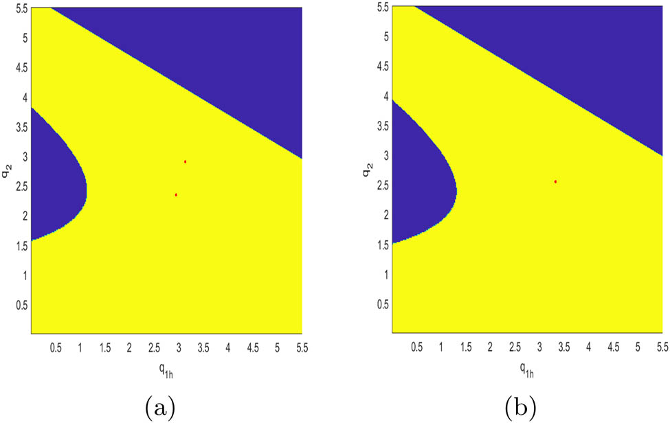
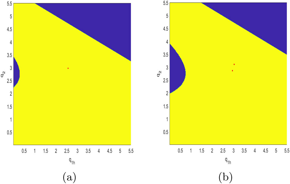
Figures 15, 16, 17, 18, 19, and 20 simulate the attraction basin of system (10) with different values of
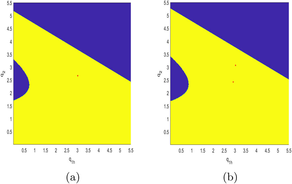
The attraction basin of system (10) with different values of θ. (a) θ = 0.2; (b) θ = 0.6.
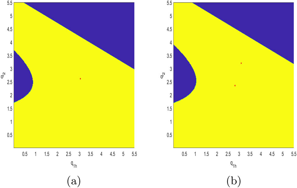
The attraction basin of system (10) with different values of γ. (a) γ = 0.1; (b) γ = 0.6.
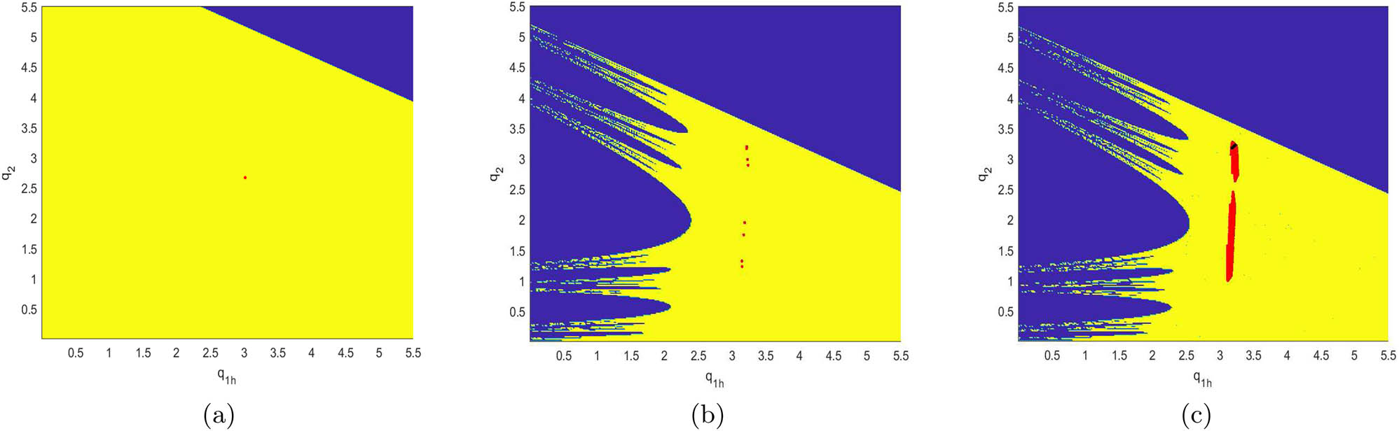
The attraction basin of system (10) with different values of v. (a) v = 0.2; (b) v = 0.49; (c) v = 0.505.
The attraction basin of system (10) with different values of β 2. (a) β 2 = 0.05; (b) β 2 = 0.4; (c) β 2 = 0.9; (d) β 2 = 0.99.
The attraction basin of system (10) with different values of
The attraction basin of system (10) with different values of
5 Chaos control
In a chaotic market, the product outputs can not be predicted, which is not conducive to the long-term development of cluster enterprises. Therefore, it is necessary to adopt corresponding methods and measures to rid the market of chaos. Prior literature shows that parameter variation and feedback are two effective methods to control chaos [10,12, 13,19,20,38–42]. A state variables feedback and parameter variation method was proposed [43] and had been used in many works [44–46], and it will applied in our article. Hence, the three-dimensional discrete dynamic system (10) are changed into the following format:
where
From Figure 4, system (10) falls into chaos when
The bifurcation diagram of the system (13) with respect to the controlling factor
The time series of system (13) when control parameter
In the real word, as well as the theoretical analysis of Section 3, we can vary parameters to maintain the stability of outputs, for example, increasing the adjustment speed of firms with uncertain cost, slowing the adjustment speed of firms with transparent cost, reducing R&D spillovers, increasing TIE of firms with uncertain cost, and so on. As described in system (13) and verified in Figures 21 and 22, another way to obtain the market out of mess is that, the outputs adjustment in the next period should takes more account of the outputs in current period.
6 Conclusion
It is an attractive topic to study dynamic games with imperfect rationality and incomplete information, which scholars paid less attention. In this article, a dynamic duopoly Cournot model with asymmetric information and bounded rationality is constructed, where two firms adopt different output adjustment strategies. We introduce two important realistic assumptions into our model, the first is that firms have different R&D capabilities, R&D spillovers only flow from firm 1 with stronger R&D capabilities to firm 2 with weaker R&D capabilities by one-way. The second is the information asymmetry between these two firms, that is, firm 2’s marginal cost is well known, while firm 1’s marginal cost is a private information.
We discuss the existence and the stability of Bayesian Nash equilibrium in discrete systems with heterogenous expectations in two cases, and interestingly, we obtain two opposite findings. In the first case, where firms adopt adaptive expectation and naïve expectation, it is found that firms’ outputs are always stable no matter what the values of other model parameters are. In the second case, where firms use adaptive expectation and gradient dynamical expectation, equilibrium points are locally asymptotically stable only when the model parameters met certain conditions, the dynamic system could go from equilibrium to bifurcation, or from unstable state to steady with model parameters varying. In particular, when the probability of high cost or technology spillovers of firm 1 is larger, the system is more likely to be away from equilibrium. When firm 1’s TIE is larger than firm 2’s, it would enlarge the stability of dynamic output system as R&D investment increases; on the contrary, it would decrease.
The numerical simulation verifies our theoretical analysis, and we describes the dynamic system via calculating the largest Lyapunov exponents, 2D bifurcation diagram, attractor basin, and sensitive dependence on initial conditions. Moreover, we stabilize the chaotic behavior of the system to a stable fixed point by introducing an appropriate controlling parameter with the state variables feedback and parameter variation method.
Acknowledgments
The authors would like to thank the reviewers and editor for their careful reading and helpful comments on the revision of paper.
-
Funding information: Science and Technology Research Project of Chongqing Municipal Education Commission (Grant No. KJQN202000832), Humanities and Social Sciences Project of the Ministry of Education (Grant No. 21YJC630130), Humanities and Social Sciences Research Major Project of Anhui Province University (Grant No. 2022AH040133), High-level Talents Program of Chongqing Technology and Business University (Grant No. 1955046), and On-campus Scientific Research Project of Chongqing Technology and Business University (Grant No. 2151018).
-
Author contributions: Jianjun Long was responsible for formulating the method, performing numerical simulation, and drafting the manuscript; and Fenglian Wang for supervising the research and revising and finalising the manuscript.
-
Conflict of interest: The authors state no conflict of interest.
-
Data availability statement: The data used to support the findings of this study are available from the corresponding author upon request. No conflict of interest exits in the this article. This article has not been copy-righted, or submitted for publication elsewhere.
Appendix A Proofs of Propositions
Proof of Proposition 1
Proposition 1 is proved if neither
Case 1: if
Case 2: if
Finally,
Proof of Proposition 2
Firstly, if
Second, from Eq. (3), when
so Eq. (7) establishes. That means we only need to verify that
Thus, Proposition 2 is proved on the hypothesis of Eq. (1).
Proof of Proposition 3
To illustrate the stability of
The characteristic polynomial of
Therefore, we can easily obtain three characteristic roots of
Thus, the Bayesian Nash equilibrium
Proof of Proposition 5
The Jacobian matrix at boundary equilibrium
The characteristic polynomial of
Apparently
References
[1] Cournot AA. Researches into the mathematical principles of the theory of wealth. Paris, France: Hachette; 1838. Search in Google Scholar
[2] Cao Z, Wang Y, Zhao J, Min J. Store brand introduction and quantity decision under asymmetric cost information in a retailer-led supply chain. Comput Industr Eng. 2021;152:106995. 10.1016/j.cie.2020.106995Search in Google Scholar
[3] Long J, Zhao H. Stability of equilibrium prices in a dynamic Duopoly Bertrand game with asymmetric information and cluster spillovers. Int J Bifurcat Chaos. 2021;31:2150240. 10.1142/S0218127421502400Search in Google Scholar
[4] Burnetas A, Gilbert SM, Smith CE. Quantity discounts in single-period supply contracts with asymmetric demand information. IIE Trans. 2007;39(5):465–79. 10.1080/07408170600941599Search in Google Scholar
[5] Chen K, Xu R, Fang H. Information disclosure model under supply chain competition with asymmetric demand disruption. Asia-Pacific J Oper Res. 2016;33(6):1–35. 10.1142/S0217595916500433Search in Google Scholar
[6] Ni J, Zhao J, Chu LK. Supply contracting and process innovation in a dynamic supply chain with information asymmetry. Eur J Oper Res. 2021;288(2):552–62. 10.1016/j.ejor.2020.06.008Search in Google Scholar
[7] Etro F, Cella M. Equilibrium principal-agent contracts: competition and R&D incentives. J Econ Manag Strategy. 2013;22(3):488–512. 10.1111/jems.12021Search in Google Scholar
[8] Baumol WJ, Quandt RE. Rules of thumb and optimally imperfect decisions. Amer Econ Rev. 1964;54(2):23–46. Search in Google Scholar
[9] Bischi GI, Lamantia F. Nonlinear duopoly games with positive cost externalities due to spillover effects. Chaos Solitons Fractals. 2002;13(4):805–22. 10.1016/S0960-0779(01)00006-6Search in Google Scholar
[10] Elsadany AA, Awad AM. Dynamical analysis and chaos control in a heterogeneous Kopel duopoly game. Indian J Pure Appl Math. 2016;47(4):617–39. 10.1007/s13226-016-0206-3Search in Google Scholar
[11] Long J, Huang H. A dynamic Stackelberg-Cournot Duopoly model with heterogeneous strategies through one-way spillovers. Discrete Dyn Nature Soc. 2020 Oct;2020:1–11. 10.1155/2020/3251609Search in Google Scholar
[12] Ding J, Mei Q, Yao H. Dynamics and adaptive control of a Duopoly advertising model based on heterogeneous expectations. Nonlinear Dyn. 2012;67(1):129–38. 10.1007/s11071-011-9964-ySearch in Google Scholar
[13] Bai M, Gao Y. Chaos control on a Duopoly game with homogeneous strategy. Discrete Dyn Nature Soc. 2016;2016(1):1–7. 10.1155/2016/7418252Search in Google Scholar
[14] Askar SS, Simos T. Tripoly Stackelberg game model: One leader versus two followers. Appl Math Comput. 2018;328:301–11. 10.1016/j.amc.2018.01.041Search in Google Scholar
[15] Peng Y, Lu Q, Wu X, Zhao Y, Xiao Y. Dynamics of Hotelling triopoly model with bounded rationality. Appl Math Comput. 2020;373:12507. 10.1016/j.amc.2019.125027Search in Google Scholar
[16] Bischi GI, Naimzada AK, Sbragia L. Oligopoly games with local monopolistic approximation. J Econ Behav Organ. 2007;62(3):371–88. 10.1016/j.jebo.2005.08.006Search in Google Scholar
[17] Elsadany AA. A dynamic Cournot duopoly model with different strategies. J Egyptian Math Soc. 2015;23(1):56–61. 10.1016/j.joems.2014.01.006Search in Google Scholar
[18] Askar SS, Alnowibet K. Nonlinear oligopolistic game with isoelastic demand function: Rationality and local monopolistic approximation. Chaos Solitons Fractals. 2016;84:15–22. 10.1016/j.chaos.2015.12.019Search in Google Scholar
[19] Tesoriere A. Endogenous R&D symmetry in linear duopoly with one-way spillovers. J Econ Behav Organ. 2006;66(2):213–25. 10.1016/j.jebo.2006.04.007Search in Google Scholar
[20] D’Aspremont C, Jacquemin A. Cooperative and noncooperative R&D in Duopoly with spillovers. Amer Econ Rev. 1988;78(5):1133–7. Search in Google Scholar
[21] Bischi GI, Lamantia F. A dynamic model of oligopoly with R&D externalities along networks: Part I. Math Comput Simulat. 2012;84:51–65. 10.1016/j.matcom.2012.08.006Search in Google Scholar
[22] Li T, Ma J. The complex dynamics of R&D competition models of three oligarchs with heterogeneous players. Nonlinear Dyn. 2013;74(1–2):45–54. 10.1007/s11071-013-0947-zSearch in Google Scholar
[23] Tu H, Wang X. Complex dynamics and control of a dynamic R&D Bertrand triopoly game model with bounded rational rule. Nonlinear Dyn. 2017;88(1):703–14. 10.1007/s11071-016-3271-6Search in Google Scholar
[24] Zhou J, Zhou W, Chu T, Chang Y, Huang M. Bifurcation, intermittent chaos and multi-stability in a two-stage Cournot game with R&D spillover and product differentiation. Appl Math Comput. 2019;341:358–78. 10.1016/j.amc.2018.09.004Search in Google Scholar
[25] Porter M. Competitive advantage of nations. New York (NY), USA: The Free Press; 1998. 10.1007/978-1-349-14865-3Search in Google Scholar
[26] Li L. Multi-dimensional proximities and industrial cluster innovation. Beijing, China: Peking University Press; 2014. Search in Google Scholar
[27] Boccard N, Wauthy XY. Bertrand competition and cournot outcomes. Econ Lett. 2000 Sep;68:279–85. 10.1016/S0165-1765(00)00256-1Search in Google Scholar
[28] Ushio Y. Welfare effects of commodity taxation in cournot oligopoly. Jpn Econ Rev. 2002 Dec;51:268–73. 10.1111/1468-5876.00151Search in Google Scholar
[29] Elabbasy EM, Agiza HN, Elsadany AA. Analysis of nonlinear triopoly game with heterogeneous players. Comput Math Appl. 2009;57(3):488–99. 10.1016/j.camwa.2008.09.046Search in Google Scholar
[30] Ding Z, Li Q, Jiang S, Wang X. Dynamics in a Cournot investment game with heterogeneous players. Appl Math Comput. 2015;256:939–50. 10.1016/j.amc.2015.01.060Search in Google Scholar
[31] Elsadany AA. Dynamics of a Cournot duopoly game with bounded rationality based on relative profit maximization. Appl Math Comput. 2017;294:253–63. 10.1016/j.amc.2016.09.018Search in Google Scholar
[32] Rand D. Exotic phenomena in games and duopoly models. J Math Econ. 1978;5(2):173–84. 10.1016/0304-4068(78)90022-8Search in Google Scholar
[33] Yi Q, Zeng X. Complex dynamics and chaos control of duopoly Bertrand model in Chinese air-conditioning market. Chaos Solitons Fractals. 2015;76:231–7. 10.1016/j.chaos.2015.04.008Search in Google Scholar
[34] Long J, Huang H. Stability of equilibrium production-price in a dynamic duopoly Cournot-Bertrand game with asymmetric information and cluster spillovers. Math Biosci Eng. 2022;19(12):14056–73. 10.3934/mbe.2022654Search in Google Scholar PubMed
[35] Bischi GI, Lamantia F. A dynamic model of oligopoly with R&D externalities along networks. Part II. Math Comput Simulat. 2012;84:66–82. 10.1016/j.matcom.2012.09.001Search in Google Scholar
[36] Yu W, Yu Y. The stability of Bayesian Nash equilibrium of dynamic Cournot duopoly model with asymmetric information. Commun Nonlinear Sci Numer Simulat. 2018;63:101–16. 10.1016/j.cnsns.2018.03.001Search in Google Scholar
[37] Gibbons R. Game theory for applied economists. Princeton (NJ), USA: Princeton University Press; 2010. Search in Google Scholar
[38] Du JG, Huang T, Sheng Z. Analysis of decision-making in economic chaos control. Nonlinear Anal Real World Appl. 2009;10(4):2493–501. 10.1016/j.nonrwa.2008.05.007Search in Google Scholar
[39] Kaas L. Stabilizing chaos in a dynamic macroeconomic model. J Econ Behav Organ. 1998;33(3–4):313–32. 10.1016/S0167-2681(97)00061-9Search in Google Scholar
[40] Agiza HN. On the analysis of stability, bifurcation, chaos and chaos control of Kopel map. Chaos Solitons Fractals. 1999;10(11):1909–16. 10.1016/S0960-0779(98)00210-0Search in Google Scholar
[41] Holllyst JA, Urbanowicz K. Chaos control in economical model by time-delayed feedback method. Physica A. 2012;287(3):587–98. 10.1016/S0378-4371(00)00395-2Search in Google Scholar
[42] Amer YA. Resonance and vibration control of two-degree-of-freedom nonlinear electromechanical system with harmonic excitation. Nonlinear Dyn. 2015;81(4):2003–19. 10.1007/s11071-015-2121-2Search in Google Scholar
[43] Luo XS, Chen G, Wang BH, Fang JQ. Hybrid control of period-doubling bifurcation and chaos in discrete nonlinear dynamical systems. Chaos Solitons Fractals. 2003;18(4):775–83. 10.1016/S0960-0779(03)00028-6Search in Google Scholar
[44] Peng Y, Lu Q, Xiao Y. A dynamic Stackelberg duopoly model with different strategies. Chaos Solitons Fractals. 2016;85:128–34. 10.1016/j.chaos.2016.01.024Search in Google Scholar
[45] Peng Y, Lu Q, Xiao Y, Wu X. Complex dynamics analysis for a remanufacturing duopoly model with nonlinear cost. Physica A. 2019;514:658–70. 10.1016/j.physa.2018.09.143Search in Google Scholar
[46] Pu X, Ma J. Complex dynamics and chaos control in nonlinear four-oligopolist game with different expectations. Int J Bifurcat Chaos. 2013;23(3):1350053. 10.1142/S0218127413500533Search in Google Scholar
© 2023 the author(s), published by De Gruyter
This work is licensed under the Creative Commons Attribution 4.0 International License.
Articles in the same Issue
- Research Articles
- The regularization of spectral methods for hyperbolic Volterra integrodifferential equations with fractional power elliptic operator
- Analytical and numerical study for the generalized q-deformed sinh-Gordon equation
- Dynamics and attitude control of space-based synthetic aperture radar
- A new optimal multistep optimal homotopy asymptotic method to solve nonlinear system of two biological species
- Dynamical aspects of transient electro-osmotic flow of Burgers' fluid with zeta potential in cylindrical tube
- Self-optimization examination system based on improved particle swarm optimization
- Overlapping grid SQLM for third-grade modified nanofluid flow deformed by porous stretchable/shrinkable Riga plate
- Research on indoor localization algorithm based on time unsynchronization
- Performance evaluation and optimization of fixture adapter for oil drilling top drives
- Nonlinear adaptive sliding mode control with application to quadcopters
- Numerical simulation of Burgers’ equations via quartic HB-spline DQM
- Bond performance between recycled concrete and steel bar after high temperature
- Deformable Laplace transform and its applications
- A comparative study for the numerical approximation of 1D and 2D hyperbolic telegraph equations with UAT and UAH tension B-spline DQM
- Numerical approximations of CNLS equations via UAH tension B-spline DQM
- Nonlinear numerical simulation of bond performance between recycled concrete and corroded steel bars
- An iterative approach using Sawi transform for fractional telegraph equation in diversified dimensions
- Investigation of magnetized convection for second-grade nanofluids via Prabhakar differentiation
- Influence of the blade size on the dynamic characteristic damage identification of wind turbine blades
- Cilia and electroosmosis induced double diffusive transport of hybrid nanofluids through microchannel and entropy analysis
- Semi-analytical approximation of time-fractional telegraph equation via natural transform in Caputo derivative
- Analytical solutions of fractional couple stress fluid flow for an engineering problem
- Simulations of fractional time-derivative against proportional time-delay for solving and investigating the generalized perturbed-KdV equation
- Pricing weather derivatives in an uncertain environment
- Variational principles for a double Rayleigh beam system undergoing vibrations and connected by a nonlinear Winkler–Pasternak elastic layer
- Novel soliton structures of truncated M-fractional (4+1)-dim Fokas wave model
- Safety decision analysis of collapse accident based on “accident tree–analytic hierarchy process”
- Derivation of septic B-spline function in n-dimensional to solve n-dimensional partial differential equations
- Development of a gray box system identification model to estimate the parameters affecting traffic accidents
- Homotopy analysis method for discrete quasi-reversibility mollification method of nonhomogeneous backward heat conduction problem
- New kink-periodic and convex–concave-periodic solutions to the modified regularized long wave equation by means of modified rational trigonometric–hyperbolic functions
- Explicit Chebyshev Petrov–Galerkin scheme for time-fractional fourth-order uniform Euler–Bernoulli pinned–pinned beam equation
- NASA DART mission: A preliminary mathematical dynamical model and its nonlinear circuit emulation
- Nonlinear dynamic responses of ballasted railway tracks using concrete sleepers incorporated with reinforced fibres and pre-treated crumb rubber
- Two-component excitation governance of giant wave clusters with the partially nonlocal nonlinearity
- Bifurcation analysis and control of the valve-controlled hydraulic cylinder system
- Engineering fault intelligent monitoring system based on Internet of Things and GIS
- Traveling wave solutions of the generalized scale-invariant analog of the KdV equation by tanh–coth method
- Electric vehicle wireless charging system for the foreign object detection with the inducted coil with magnetic field variation
- Dynamical structures of wave front to the fractional generalized equal width-Burgers model via two analytic schemes: Effects of parameters and fractionality
- Theoretical and numerical analysis of nonlinear Boussinesq equation under fractal fractional derivative
- Research on the artificial control method of the gas nuclei spectrum in the small-scale experimental pool under atmospheric pressure
- Mathematical analysis of the transmission dynamics of viral infection with effective control policies via fractional derivative
- On duality principles and related convex dual formulations suitable for local and global non-convex variational optimization
- Study on the breaking characteristics of glass-like brittle materials
- The construction and development of economic education model in universities based on the spatial Durbin model
- Homoclinic breather, periodic wave, lump solution, and M-shaped rational solutions for cold bosonic atoms in a zig-zag optical lattice
- Fractional insights into Zika virus transmission: Exploring preventive measures from a dynamical perspective
- Rapid Communication
- Influence of joint flexibility on buckling analysis of free–free beams
- Special Issue: Recent trends and emergence of technology in nonlinear engineering and its applications - Part II
- Research on optimization of crane fault predictive control system based on data mining
- Nonlinear computer image scene and target information extraction based on big data technology
- Nonlinear analysis and processing of software development data under Internet of things monitoring system
- Nonlinear remote monitoring system of manipulator based on network communication technology
- Nonlinear bridge deflection monitoring and prediction system based on network communication
- Cross-modal multi-label image classification modeling and recognition based on nonlinear
- Application of nonlinear clustering optimization algorithm in web data mining of cloud computing
- Optimization of information acquisition security of broadband carrier communication based on linear equation
- A review of tiger conservation studies using nonlinear trajectory: A telemetry data approach
- Multiwireless sensors for electrical measurement based on nonlinear improved data fusion algorithm
- Realization of optimization design of electromechanical integration PLC program system based on 3D model
- Research on nonlinear tracking and evaluation of sports 3D vision action
- Analysis of bridge vibration response for identification of bridge damage using BP neural network
- Numerical analysis of vibration response of elastic tube bundle of heat exchanger based on fluid structure coupling analysis
- Establishment of nonlinear network security situational awareness model based on random forest under the background of big data
- Research and implementation of non-linear management and monitoring system for classified information network
- Study of time-fractional delayed differential equations via new integral transform-based variation iteration technique
- Exhaustive study on post effect processing of 3D image based on nonlinear digital watermarking algorithm
- A versatile dynamic noise control framework based on computer simulation and modeling
- A novel hybrid ensemble convolutional neural network for face recognition by optimizing hyperparameters
- Numerical analysis of uneven settlement of highway subgrade based on nonlinear algorithm
- Experimental design and data analysis and optimization of mechanical condition diagnosis for transformer sets
- Special Issue: Reliable and Robust Fuzzy Logic Control System for Industry 4.0
- Framework for identifying network attacks through packet inspection using machine learning
- Convolutional neural network for UAV image processing and navigation in tree plantations based on deep learning
- Analysis of multimedia technology and mobile learning in English teaching in colleges and universities
- A deep learning-based mathematical modeling strategy for classifying musical genres in musical industry
- An effective framework to improve the managerial activities in global software development
- Simulation of three-dimensional temperature field in high-frequency welding based on nonlinear finite element method
- Multi-objective optimization model of transmission error of nonlinear dynamic load of double helical gears
- Fault diagnosis of electrical equipment based on virtual simulation technology
- Application of fractional-order nonlinear equations in coordinated control of multi-agent systems
- Research on railroad locomotive driving safety assistance technology based on electromechanical coupling analysis
- Risk assessment of computer network information using a proposed approach: Fuzzy hierarchical reasoning model based on scientific inversion parallel programming
- Special Issue: Dynamic Engineering and Control Methods for the Nonlinear Systems - Part I
- The application of iterative hard threshold algorithm based on nonlinear optimal compression sensing and electronic information technology in the field of automatic control
- Equilibrium stability of dynamic duopoly Cournot game under heterogeneous strategies, asymmetric information, and one-way R&D spillovers
- Mathematical prediction model construction of network packet loss rate and nonlinear mapping user experience under the Internet of Things
- Target recognition and detection system based on sensor and nonlinear machine vision fusion
- Risk analysis of bridge ship collision based on AIS data model and nonlinear finite element
- Video face target detection and tracking algorithm based on nonlinear sequence Monte Carlo filtering technique
- Adaptive fuzzy extended state observer for a class of nonlinear systems with output constraint