Research on indoor localization algorithm based on time unsynchronization

2.1 Iterative TOA algorithm

Since the TOA-based positioning algorithm requires strict time synchronization, the accuracy requirements of the hardware are relatively strict and the cost is high. In order to reduce the influence of time asynchrony and NLOS error, Kang et al. [4,5] proposed an iterative algorithm based on TOA, first constructing a circle model equation set, and using the least squares method to linearize the nonlinear problem. Then, we construct the NLOS error matrix equation using the weighted least squares method and minimize the sum of the NLOS errors.

1. Eliminate time synchronization errors

   The coordinates of the anchor node are X M i = [ x i y i ] , the coordinates of the target node are X T = [ x y ] , and the measured distance can be modeled as:

   (1) d i = dis _ real i + e i + Δ d ,

   where dis_rea l i represents the actual distance between the anchor node i and the target node, and Δ d represents the measurement error caused by the time synchronization error.

   The approximate measurement before the anchor node and the target node can be written as:

   (2) ( d i − Δ d ) 2 = ( x − x i ) 2 + ( y − y i ) 2 .

   This can be converted to the linearized matrix form:

   (3) A θ = h ,

   where A = − 2 x 1 − 2 y 1 2 d 1 1 − 2 x 2 − 2 y 2 2 d 2 1 ⋮ ⋮ ⋮ ⋮ − 2 x n − 2 y n 2 d n 1 , θ = x y Δ d H , h = d 1 2 − k 1 d 2 2 − k 2 ⋮ d n 2 − k n , H = x 2 + y 2 − Δ d 2 k i = x i 2 + y i 2 .

   The estimate coordinates and time synchronization error can be obtained by the least squares method:

   (4) θ LS = ( A T A ) − 1 A T h .

2. Minimize the NLOS error

   The error vector corresponding to the estimated position of the target node is as follows:

   (5) V = h − A θ 0 = ( v 1 v 2 ⋯ v n ) T ,

   where θ 0 = ( x 0 y 0 Δ d 0 H ) T represents the true value of θ .

   The variance of V can be expressed as ψ = E [ V V T ] . The covariance matrix is a positive definite weighting matrix Q , and the true distance B between the anchor node to be reconstructed and the target node can be expressed as Q = P 1 0 ⋯ 0 0 P 2 ⋱ ⋮ ⋮ ⋱ ⋱ 0 0 ⋯ 0 P n and B = R 1 0 ⋯ 0 0 R 2 ⋱ ⋮ ⋮ ⋱ ⋱ 0 0 ⋯ 0 R n . Since the measurement error of NLOS is usually smaller than the actual calculated distance, the error matrix can be approximated as:

   (6) V = h − A θ 0 = d i 2 − k i + 2 x i x 0 + 2 y i y 0 − 2 d i Δ d 0 − H = ( d i − Δ d 0 ) 2 − B 2 = ( B + λ ) 2 − B 2 = 2 B λ + λ ⋅ λ ≈ 2 B λ .

   The covariance of the NLOS measurement is the same as Q ; then, the covariance matrix ψ can be expressed as ψ = E [ V V T ] = 4 BQB . Applying the weighted least squares algorithm, we obtain

   (7) θ ̇ = ( A T ψ − 1 A ) − 1 ( A T ψ − 1 h ) .

3. Iterate to obtain the final result

In practical application scenarios, the actual distance between the anchor node and the target node is unknown, and the actual distance B can only be reconstructed by measuring the distance d i . The estimated coordinates of the target node can be calculated by:

Step 1: Use the weighted least squares algorithm to obtain the initial estimation result as follows:

Step 2: Use the time synchronization error Δ d ˆ 1 to update the matrices B and A :

where d ′ i = d i − Δ d ˆ 1 , i = 1 , 2 , … , n .

Step 3: Obtain a new error matrix:

Step 4: Use the weighted least squares algorithm to obtain an improved solution:

Since the matrix B is a rough approximation of the real matrix, iteration can be employed to obtain the final result. A new calculation Δ d ˆ l can be obtained, where l = 1 , 2 , … , L , L is the number of iterations.

2.2 Linear position line algorithm

Caffery [13] proposed a new geometric interpretation in which position straight lines are used instead of circular LOPs to determine the position of the transmitter. Linear LOPs are derived from simple observations of system geometry, not linearization.

N distance equations can be expressed as: ‖ ( x i , y i ) − ( x , y ) ‖ 2 2 = R i 2 . By subtracting the reference base station, N − 1 equation can be obtained as follows:

The matrix form is Y = AX . The least squares solution is X ˆ = ( A T A ) − 1 A T Y .

2.3 CHAN algorithm

CHAN algorithm [14] was proposed in 1994. It mainly transforms the nonlinear equation into a set of linear equations with unknown parameters and intermediate variables by introducing intermediate variables. First, the initial solution is given by using the least squares algorithm, and then, the final solution of the position coordinates is given by using the weighted least squares algorithm according to the relationship between the known intermediate variables and the position coordinates. The pseudo-code of the algorithm is shown in Table 1.

2.4 Quadratic programming

The measurement model is r i = d i + Δ d + e i + n i , where d i represents the actual distance between anchor node and target node, Δ d = c × Δ t represents time synchronization error, e i represents NLOS error, and n i represents measurement noise.

To define a new vector θ 1 = [ x , y , Δ d , H ] T , you can obtain a mathematical programming problem as follows:

where ψ 1 = B 1 Q 1 B 1 , K i = x i 2 + y i 2 , B 1 = diag { 2 d 1 , ⋯ , 2 d N } , Q 1 = diag { σ 1 2 , ⋯ , σ N 2 } , H = x 2 + y 2 − Δ d 2 , A 1 = − 2 x 1 − 2 y 1 2 r 1 1 − 2 x 2 − 2 y 2 2 r 2 1 ⋮ ⋮ ⋮ ⋮ − 2 x N − 2 y N 2 r N 1 ,   h 1 = r 1 2 − k 1 r 2 2 − k 2 ⋮ r N 2 − k N .

The aforementioned form can be transformed into a standard quadratic programming form:

The aforementioned QP problems [15] can be solved by the interior point method.

2.5 QP-WLS

Wu et al. [6] based on the solution of QP problem obtained in 2019 improved it by WLS algorithm. The estimation error of x , y , Δ d , H is defined as e 1 , e 2 , e 3 , e 4 , θ 2 = [ x 2 , y 2 , Δ d 2 ] T and the reconstruction vector ε = h 2 − A 2 θ 2 ; then, the least squares solution can be expressed as:

where ψ 2 = B 2 Q 2 B 2 , B 2 = diag { 2 x , 2 y , 2 Δ d , 1 } , A 2 = 1 0 0 0 1 0 0 0 1 1 1 − 1 , h 2 = ( x + e 1 ) 2 ( y + e 2 ) 2 ( Δ d + e 3 ) 2 H + e 3 .

The target node position and synchronization error are estimated as θ ′ = [ θ T , Δ d ] T :

3.1 Simulation test of 2D single-target positioning scene

Scenario description: one target node and seven anchor nodes are randomly deployed in a 100 m × 100 m 2D site. The NLOS error follows N ( i , 0.1 ) , i = 0, 2, 4, 6 , ⋯ , and the time synchronization error is 0 m / 3 m / 6 m / 9 m / ⋯ .

1. Cumulative distribution function with NLOS error of 2 m and time synchronization error of 3 m

When the NLOS error is fixed at 2 m and the time synchronization error is fixed at 3 m, 1,000 Monte Carlo simulations are carried out for the five algorithms, and the cumulative distribution (CDF) diagram of RMSE of each algorithm is shown in Figure 1.

Figure 1

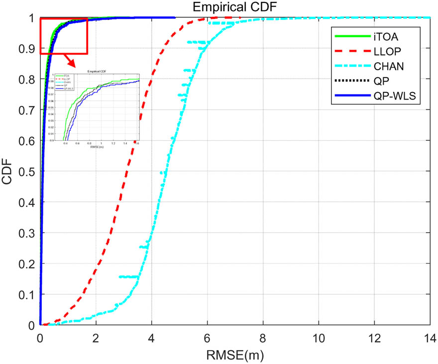
CDF of RMSE with NLOS error of 2 m and time synchronization error of 3 m.

It can be seen from Figure 1 that 90% of the RMSE data of iTOA, QP, and QP-WLS algorithms fall within 0.35, 0.44, and 0.48 m in 1,000 operations. However, 90% of the RMSE data of iTOA LLOP and CHAN algorithms fall within 4.51 and 5.97 m. It can be seen that when the NLOS error is fixed at 2 m and the time synchronization error is fixed at 3 m, the error of iTOA algorithm is relatively low.

1. Comparison of time synchronization errors under the same NLOS error value

When the NLOS error value is fixed at 2 m, the ALE of 1,000 Monte Carlo simulations performed by each algorithm under different time synchronization errors is shown in Table 2 and Figure 2.

Figure 2

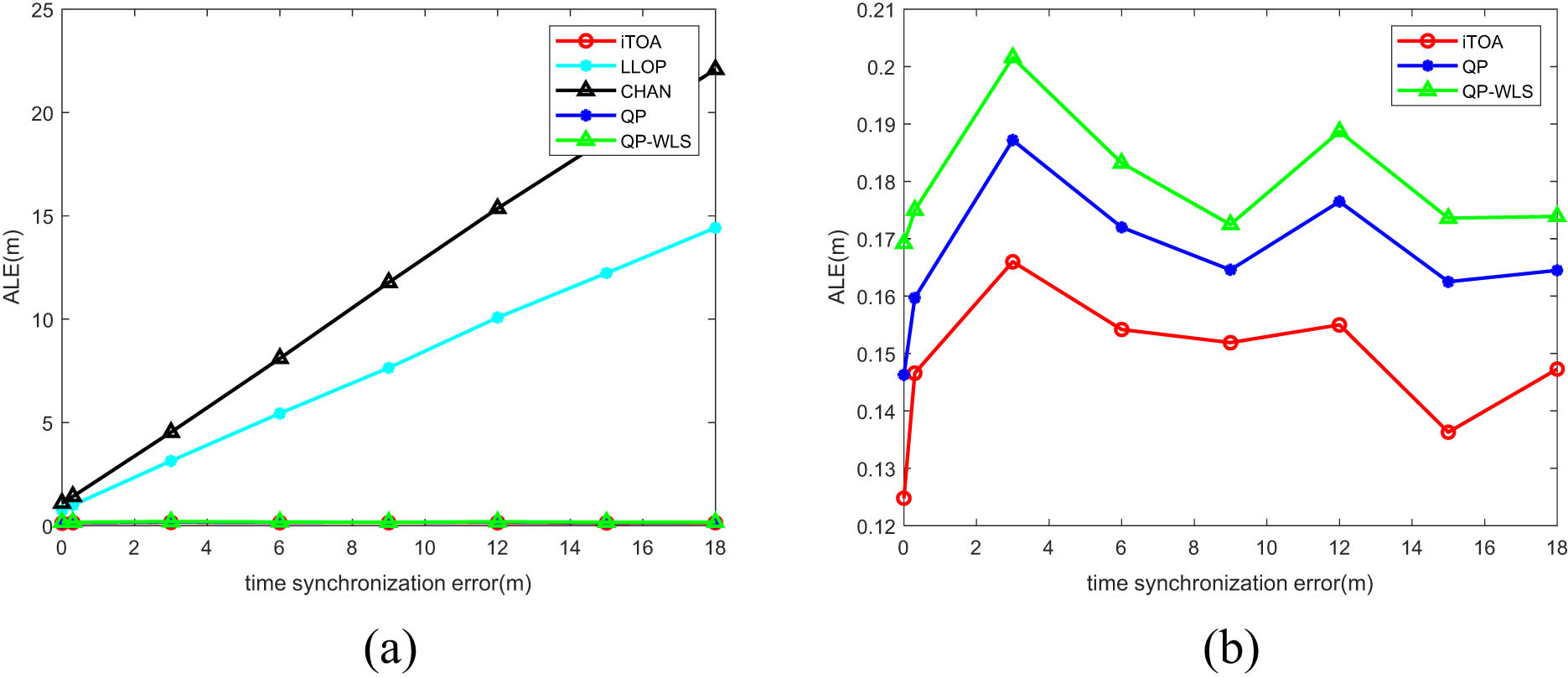
ALE of different time synchronization errors of five algorithms when the NLOS error value is fixed at 2m. (a) ALE diagram of five algorithms and (b) ALE diagram of three algorithms.

From the simulation results in Figure 2, when the NLOS error value is fixed at 2 m, comparing the positioning results under different time synchronization errors, it is found that the error of the CHAN algorithm is always the largest, and the ALE of the CHAN and LLOP algorithms changes with the time synchronization error value that increases monotonically. When the five algorithms are compared together, due to the large errors of the CHAN and LLOP algorithms, which are not in the same order of magnitude as other algorithms, the error changes of the other three algorithms are less obvious. By comparing the other three algorithms separately, it can be found that as the time synchronization error increases to 18 m, the average positioning error of each algorithm is less than 0.21 m, reaching the positioning accuracy of decimeter level, and iTOA algorithm shows the optimal positioning performance, followed by the solution of quadratic programming problem.

1. Comparison of different NLOS error values under the same time synchronization error

   When the time synchronization error is fixed at 3 m, the ALE of each algorithm for 1,000 Monte Carlo simulations under different NLOS error values is shown in Table 3 and Figure 3.

Figure 3

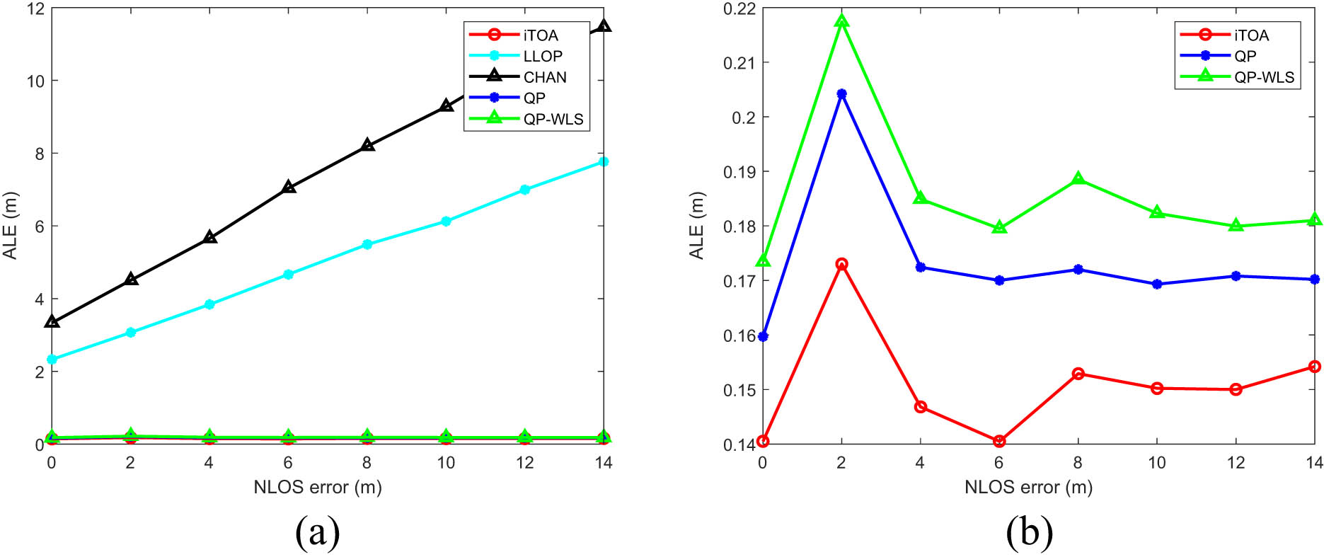
ALE of different time synchronization errors of five algorithms when the NLOS error value is fixed at 3m. (a) ALE diagram of five algorithms and (b) ALE diagram of three algorithms.

When the time synchronization error is fixed at 3 m, when comparing the positioning results of each algorithm under different NLOS error values, it is found that the error of the CHAN algorithm is still the largest. When the NLOS error value is 14 m, the average positioning error of the algorithm reaches nearly 10.6 m. The iTOA algorithm still shows the best positioning performance. When the NLOS error value is 14 m, the average positioning error of the algorithm is only 0.153 m.

3.2 Simulation test of 2D and 3D multi-target positioning scenarios

Five target nodes and ten anchor nodes are randomly generated in the 2D ( 100 m × 100 m ) and 3D ( 100 m × 100 m × 20 m ) positioning sites, and the positioning results of each algorithm when the NLOS error is 2 m and the time synchronization error is 3 m are shown in Figure 4.

Figure 4

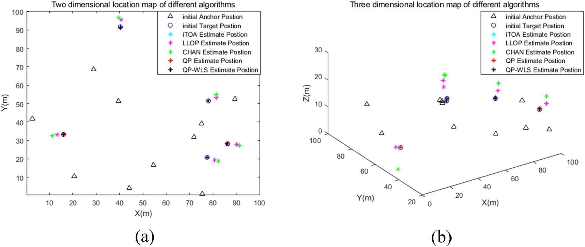
Multi-target localization scene. (a) 2D multi-target localization scene and (b) 3D multi-target localization scene.

The five different algorithms are Monte Carlo simulations 1,000 times, and the ALEs for 1,000 runs are shown in Table 4.

The CDF of the RMSE for each run is shown in Figure 5.

Figure 5

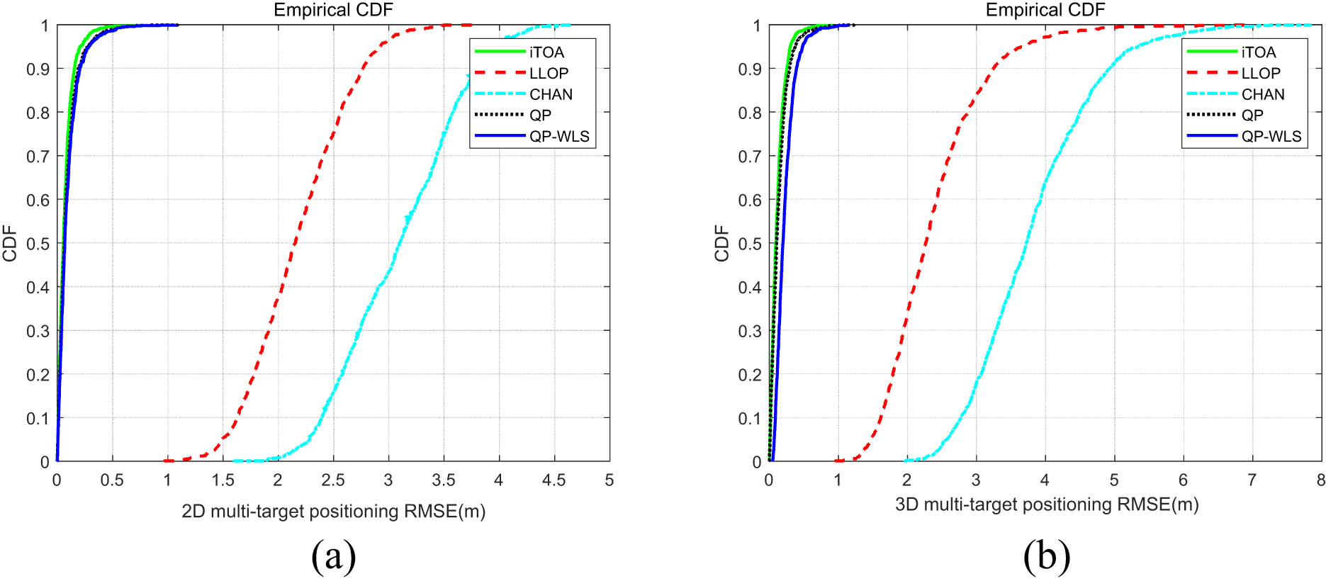
CDF of RMSE: (a) 2D CDF of RMSE and (b) 3D CDF of RMSE.

From the aforementioned simulation results, it can be seen that the positioning error of iTOA algorithm is the smallest, followed by QP and QP-WLS algorithms, whether it is extended from single-target positioning to multi-target positioning, or from 2D positioning to 3D positioning, and the error of CHAN algorithm is still the largest.

3.3 Simulation test considering clock offset and clock skew

The accuracy of computer clock depends on the accuracy of crystal oscillator frequency. Due to process and material reasons, the actual frequency of quartz crystals with the same nominal frequency on the same production line is different. The function of crystal oscillator is to provide basic clock signal for the system. Wang et al. [12] believed that the lack of synchronization on nodes may be attributed to each node having a unique clock, which means that the clock tilt and offset of each node are different. Local time of nodes can be modeled as:

where F i ( t ) indicates the local time, t indicates the ideal time, 1 + ε i indicates the clock skew, and ς i indicates the clock offset.

In addition to considering clock offset, clock skew, NLOS error ratio, and time synchronization error ratio, this section also compares the simulation tests of five algorithms in four scenarios. The first scenario is that there is a sight distance between the anchor node and the target node and there is no noise. The second scenario is that there are NLOS errors and time synchronization errors between the anchor node and the target node, and the error values are the same. The third scenario is that there are partial NLOS and time synchronization errors (proportionally) between the anchor node and the target node, and the total error has the same impact on different nodes. The fourth scenario is that there are partial NLOS and time synchronization errors between the anchor node and the target node, and the total error has different effects on different nodes. Note: Scenarios 2–4 are affected by noise.

The first scenario is set to test whether the algorithm itself has problems. If the error of each algorithm is large without the influence of any error and noise, it indicates that the algorithm itself has problems. The second scenario and the third scenario can be used to compare the positioning accuracy of each algorithm when the proportion of time synchronization error and NLOS error is different. The third scenario and the fourth scenario can be used to compare the positioning accuracy of each algorithm when the proportion of time synchronization error and NLOS error is the same, but the error value is different.

When the time synchronization error accounts for 20% and NLOS error accounts for 0%, time synchronization error accounts for 20% and NLOS error accounts for 30%. Time synchronization error accounts for 50% and NLOS error accounts for 50%. When the time synchronization error accounts for 90% and the NLOS error accounts for 90%, the average positioning error results of the five algorithms running 1,000 times independently in four scenarios are shown in Figure 6.

Figure 6

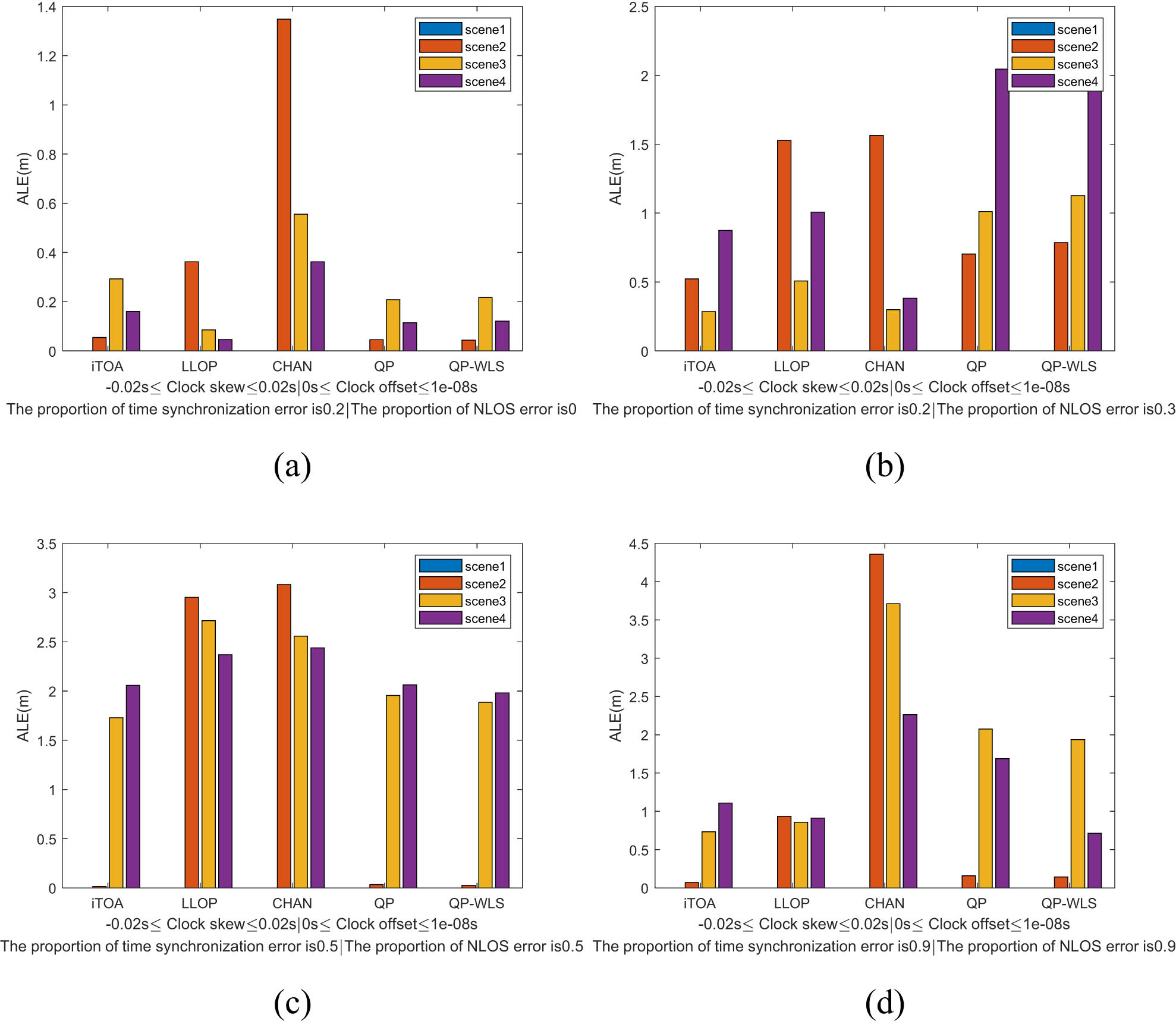
Average positioning error diagram of each algorithm when the proportion of time synchronization error and NLOS error is different. (a) The proportion of time synchronization error is 0; (b) The proportion of time synchronization error is 0.3; (c) The proportion of time synchronization error is 0.5; (d) The proportion of time synchronization error is 0.9.

Among them, the abscissa represents each algorithm, the ordinate represents the average positioning error of each algorithm running 1,000 times in each scenario, and different colors represent different scenarios. The data of Scenario 1 are not displayed, indicating that the average positioning error of the algorithm is also 0 when there is no time synchronization error and NLOS error, which further confirms that there is no problem in the design of these five algorithms. Comparing the second and third scenarios, it can be seen that with the reduction of the time synchronization error and the proportion of NLOS error, the average positioning errors of the LLOP algorithm and the CHAN algorithm have decreased, while the QP algorithm and the QP-WLS algorithm have increased instead. Comparing the third scenario and the fourth scenario, it is found that when the error has the same impact on nodes, iTOA algorithm has a better positioning effect. Overall, comparing the five algorithms, the iTOA algorithm still shows the best positioning performance, and the CHAN algorithm has the lowest positioning accuracy.

References

[1] Xu C, Wang Z, Wang Y, Wang Z, Yu L. Three passive TDOA-AOA receivers-based flying-UAV positioning in extreme environments. IEEE Sens J. 2020;20(16):9589–95.10.1109/JSEN.2020.2988920Search in Google Scholar
[2] Cao S, Chen X, Zhang X, Chen X. Combined weighted method for TDOA-based localization. IEEE Trans Instrum Meas. 2020;69(5):1962–71.10.1109/TIM.2019.2921439Search in Google Scholar
[3] Jondhale SR, Maheswar R, Lloret J. Received signal strength based target localization and tracking using wireless sensor network. EAI/Springer Innovations in Communication and Computing series. Berlin, Germany: Springer International Publishing; 2022. 10.1007/978-3-030-74061-0.Search in Google Scholar
[4] Kang YM, Wang JW. A high-precision TOA-based localization algorithm without the restriction of strict time synchronization for wireless systems. 2016 IEEE 13th International Conference on Signal Processing. (ICSP); 2016 Nov 6–10; Chengdu, China. IEEE, 2017. p. 1666–70.Search in Google Scholar
[5] Kang Y, Wang Q, Wang J, Chen R. A high-accuracy TOA-based localization method without time synchronization in a three-dimensional space. IEEE Trans Ind Inform. 2019;15(1):173–82.10.1109/TII.2018.2800047Search in Google Scholar
[6] Wu S, Zhang S, Huang D. A TOA-based localization algorithm with simultaneous NLOS mitigation and synchronization error elimination. IEEE Sens Lett. 2019;3(3):1–4.10.1109/LSENS.2019.2897924Search in Google Scholar
[7] Tian Q, Feng DZ, Hu HS. Constrained weighted least squares algorithm for TOA-based joint synchronization and localization. J Xidian Univ. 2019;46(5):1–7.Search in Google Scholar
[8] Elnahas O, Ma Y, Jiang Y, Quan Z. Clock synchronization in wireless networks using matrix completion-based maximum likelihood estimation. IEEE Trans Wirel Commun. 2020;19(12):8220–31.10.1109/TWC.2020.3020191Search in Google Scholar
[9] Yuan W, Wu N, Etzlinger B, Wang H, Kuang J. Cooperative joint localization and clock synchronization based on Gaussian message passing in asynchronous wireless networks. IEEE Trans Veh Technol. 2016;65(9):7258–73.10.1109/TVT.2016.2518185Search in Google Scholar
[10] Ma FH, Liu ZM, Guo FC. Direct position determination in asynchronous sensor networks. IEEE Trans Veh Technol. 2019;68(9):8790–803.10.1109/TVT.2019.2928638Search in Google Scholar
[11] Zou YB, Liu HP. Semidefinite programming methods for alleviating clock synchronization bias and sensor position errors in TDOA localization. IEEE Signal Process Lett. 2020;27:241–5.10.1109/LSP.2020.2965822Search in Google Scholar
[12] Wang T, Xiong H, Ding H, Zheng L. TDOA-based joint synchronization and localization algorithm for asynchronous wireless sensor networks. IEEE Trans Commun. 2020;68(5):3107–24.10.1109/TCOMM.2020.2973961Search in Google Scholar
[13] Caffery JJ. A new approach to the geometry of TOA location. Vehicular Technology Conference Fall 2000. IEEE VTS Fall VTC2000. 52nd Vehicular Technology Conference; 2000 Sep 20–24; Boston (MA), USA. IEEE, 2002. p. 1943–9.10.1109/VETECF.2000.886153Search in Google Scholar
[14] Chan YT, Ho KC. A simple and efficient estimator for hyperbolic location. IEEE Trans Signal Process. 1994;42(8):1905–15.10.1109/78.301830Search in Google Scholar
[15] Wang X, Wang ZX, O’Dea B. A TOA based location algorithm reducing the errors due to non-line-of-sight (NLOS) propagation. IEEE Trans Veh Technol. Jan. 2003;52(1):112–6.10.1109/TVT.2002.807158Search in Google Scholar
© 2023 the author(s), published by De Gruyter
This work is licensed under the Creative Commons Attribution 4.0 International License.
Articles in the same Issue
- Research Articles
- The regularization of spectral methods for hyperbolic Volterra integrodifferential equations with fractional power elliptic operator
- Analytical and numerical study for the generalized q-deformed sinh-Gordon equation
- Dynamics and attitude control of space-based synthetic aperture radar
- A new optimal multistep optimal homotopy asymptotic method to solve nonlinear system of two biological species
- Dynamical aspects of transient electro-osmotic flow of Burgers' fluid with zeta potential in cylindrical tube
- Self-optimization examination system based on improved particle swarm optimization
- Overlapping grid SQLM for third-grade modified nanofluid flow deformed by porous stretchable/shrinkable Riga plate