Homotopy analysis method for discrete quasi-reversibility mollification method of nonhomogeneous backward heat conduction problem

Mostafa Rahimi; Davood Rostamy

doi:10.1515/nleng-2022-0304

Article Open Access

Homotopy analysis method for discrete quasi-reversibility mollification method of nonhomogeneous backward heat conduction problem

Mostafa Rahimi and Davood Rostamy

Published/Copyright: July 27, 2023

Published by

Become an author with De Gruyter Brill

Submit Manuscript Author Information

From the journal Nonlinear Engineering Volume 12 Issue 1

Abstract

In this article, the inverse time problem is investigated. Regarding the ill-posed linear problem, utilize the quasi-reversibility method first. This problem has been regularized and after that provides an iterative regularizing strategy for noisy input data that are based on homotopy. For the regularizing solution, the error analysis is proved when we employ noisy measurement data as our initial guess. Finally, numerical implementations are presented.

Keywords: heat conduction; backward conduction; ill-posed problem; homotopy analysis method; quasi-reversibility; discrete mollification

1 Introduction

Take into consideration the issue of determining the temperature for a positive real number v ( x , t ) such that

(1.1) v t = v x x + f ( x , t ) , ( x , t ) ∈ ( 0 , π ) × ( 0 , T ) v ( 0 , t ) = v ( π , t ) = 0 , t ∈ [ 0 , T ] v ( x , 0 ) = g ( x ) ,

where f ( x , t ) represents the identified heat source and g ( x ) represents the starting temperature. We assume that the actual field at time t = T created by Eq. (1.1) from an unidentified initial distribution, g ( x ) ∈ L 2 ( 0 , π ) , is v [ g ] ( x , T ) = φ ( x ) . The noisy discrete data of φ ( x j ) on k = { x j , j = 1 , 2 , … , M } ⊆ [ 0 , π ] indicated by φ δ ( x j ) , are now provided to us as follows:

(1.2) ∥ φ δ − φ ∥ ∞ , [ 0 , π ] ≤ δ .

However, across several engineering disciplines like archeology and environmental science, we must take into consideration the “backward problem.” Instead of giving the initial state g ( x ) , we search v ( x , t ) for 0 ≤ t ≤ T to need to determine the generalization or its noisy measurement of a physical quantity for the final time T > 0 . They are in the category of ill-posed PDE problems in mathematics. In their research, Denche and Bessila [1] and Huang and Zheng [2] solved backward problems by regularizing techniques. As is well known, this problem is very ill-posed, i.e. sometimes there are no solutions, and when they do, they would not be continuously on the final data. In fact, small noise in the initial value tends to large error. This makes doing numerical calculations with erroneous data challenging. A regularization is therefore necessary. In the recent decades, several authors have considered the homogeneous problem that arises when f = 0 . Huang and Quan [3] approximated by perturbing the operator. This strategy is known as the quasi-reversibility method. The fundamental tenet of this approach is that a well-posed problem can be created by perturbing the equation in an ill-posed problem. Backward heat problem in the non-homogeneous situation has been approached by Dang and Nguyen [4] using quasi-reversibility to approximate Eq. (1.1). The quasi-reverse technique is the primary defense for these issues [1,2,5]. There is a wealth of literature on the issues of the past. The regularizing solution’s convergence analysis is taken into consideration in some research [1,2,6,7] together with the backward issue with the general abstract equation d v ( t ) d t + A v ( t ) = 0 . Several authors have thought about this issue in the past few decades. Lattes and Lions [8], Miller [9], and others replaced the operator A by perturbation. The ill-posed problems can be solved by perturbing the equation, one may obtain a well-posed problem. Lattes and Lions [8] added a “corrector” to the primary equation in order to regularize the issue. Huang and Zheng [2] solved this problem for the regularizing theory in the Banach space and introduced the concept of the quasi-reversibility regularization approach. Currently, a variety of inverse problems have been researched using quasi-reversibility regularization methods [10–13].

However, the homotopy analysis method (HAM) has recently been offered as a way to iteratively address various PDE problems, as evidenced in few studies [14–17]. Demonstrating strong results in resolving numerous engineering issues, both the functional characterizing the problem and the artificially induced homotopy transform have a significant impact on the convergence at p = 1 , see [16,18] for more information. In addition, it has been discovered that various inverse problems can be resolved using HAM schemes, see [17,19,20]. The two primary study areas are the design of regularizing solutions for noisy input data that can approximate the exact physical value and conditional stability for stable calculations. The approximate error bounds, roughly speaking, rely on both the regularizing techniques and a priori assumptions on the exact initial value g ( x ) .

In this article, we proposed a scheme based on the homotopy iteration to specify v ( x , t ) in 0 ≤ t < T straightforward from the final exact data φ ( x ) or noisy data φ δ ( x ) without having to initial value g ( x ) . Now, we suppose the inverse problem is in the following form:

(1.3) v t = v x x + f ( x , t ) , ( x , t ) ∈ ( 0 , π ) × ( 0 , T ) v ( 0 , t ) = v ( π , t ) = 0 , t ∈ [ 0 , T ] v ( x , T ) = φ ( x ) .

Due to the ill-posedness and for overcoming this difficulty, we regularize to approximate problem (1.3) with the quasi-reversibility method, then we reconstruct HAM for the new regularizing problem. Finally, we obtain error estimates on the approximate solution.

The remainder of this article is structured as follows: in Section 2, we reconstruct HAM after the quasi-reversibility of problem (1.3). In Section 3, we utilize this iteration approach with noisy data φ δ ( x ) and supplying the error estimates for an iterative solution; in Section 4, we provide an overview of backward piecewise homotopy analysis method (BPHAM) [21]; and in Section 5, we demonstrate the viability of the suggested approach with some numerical implementation and compare the results of our scheme in this article with the results of the BPHAM method [21].

2 Homotopy scheme and iteration process for quasi-reversibility problem

Quasi-reversibility method is a regularization idea for analysing the stability of different ill-posed problems (see [4] and the references cited therein). In this section, we approximate the issue using quasi-reversibility method to approximate Eq. (1.3) as follows [4]:

(2.1) v t − v x x − ε v x x x x = ∑ n = 1 ∞ e − ε n 4 ( T − t ) f n ( t ) sin n x , 0 ≤ x ≤ π , 0 < t < T v ( 0 , t ) = v ( π , t ) = v x x ( 0 , t ) = v x x ( π , t ) = 0 , 0 < t < T v ( x , T ) = φ ( x ) , x ∈ [ 0 , π ] ,

where ε is a positive parameter,

f n ( t ) = 2 π ⟨ f ( x , t ) , sin ( n x ) ⟩ = 2 π ∫ 0 π f ( x , t ) sin ( n x ) d x ,

and ⟨ . , . ⟩ is the inner product in L 2 ( 0 , π ) . Furthermore, we define and provide information on the homotopy scheme and its iteration process. We suggest for a more through introduction and evidence of the findings [22]. For solving Eq. (2.1), we define the following function space:

D φ = { v ( x , t ) ∈ C 2 , 1 ( ( 0 , π ) × ( 0 , T ) ) : v ( 0 , t ) = v ( π , t ) = v x x ( 0 , t ) = v x x ( π , t ) = 0 , v ( x , T ) = φ ( x ) } .

As a power series, we explicitly extend the function ϕ ( x , t ; p ) in terms of p ,

(2.2) ϕ ( x , t ; p ) = ϕ ( x , t ; 0 ) + ∑ m = 1 ∞ 1 m ! ∂ m ϕ ∂ p m = v 0 ( x , t ) + ∑ m = 1 ∞ v m ( x , t ) p m .

We specify the linear homogeneous operator in terms of v ( x , t ) ∈ D φ ,

(2.3) L [ v ] ( x , t ) = v t ( x , t ) − v x x ( x , t ) − ε v x x x x ( x , t ) .

Utilizing p ∈ [ 0 , 1 ] as the embedding parameter, we create an equation family as follows:

(2.4) ( 1 − p ) L [ ϕ ( x , t ; p ) − v 0 ( x , t ) ] = h p ( L [ ϕ ( x , t ; p ) − f ( x , t ) ] ) ,

where f ( x , t ) = ∑ n = 1 ∞ e − ε n 4 ( T − t ) f n ( t ) sin ( n x ) . From Eq. (2.4), we know

(2.5) ϕ ( x , t ; 0 ) = v 0 ( x , t ) , ϕ ( x , t ; 1 ) = v ( x , t ) ,

i.e. v 0 ( x . t ) ∈ D φ as the initial guess.

It is important to note that the auxiliary linear operator L determines the zero-order deformation equation (2.4), with the first estimate v 0 ( x , t ) , and h ∈ ( − 1 , 0 ) being an auxiliary parameter that is nonzero, hence we write

(2.6) v ( x , t ) = ϕ ( x , t ; 1 ) = v 0 ( x , t ) + ∑ m = 1 ∞ v m ( x , t ) .

We take

(2.7) v m ( x , t ) ∈ D 0 , m = 1 , 2 , … .

Subsequently, an iteration strategy for obtaining the exact solution v ( x , t ) from the sequence { v m ( x , t ) : m = 1 , 2 , 3 , … } is represented by Eqs. (2.6) and (2.7). To determine v m ( x , t ) for m = 1 , 2 , 3 , … , we use

(2.8) ( 1 − p ) ∑ m = 1 ∞ L [ v m ] ( x , t ) p m = h p ∑ m = 0 ∞ L [ v m ] ( x , t ) p m − ∑ n = 1 ∞ e − ε n 4 ( T − t ) f n ( t ) sin ( n x ) .

From Eq. (2.8), we obtain

(2.9) L [ v m − X m − 1 v m − 1 ] ( x , t ) = h L [ v m − 1 ] ( x , t ) − h ( 1 − X m − 1 ) ∑ n = 1 ∞ e − ε n 4 ( T − t ) f n ( t ) sin ( n x ) .

For m = 1 , 2 , … . , we define

(2.10) V m ( x , t ) = v m ( x , t ) − X m − 1 v m − 1 ( x , t ) , m = 2 , 3 , 4 , … ,

where X 0 = 0 and X m = 1 , v m ∈ D 0 . From Eq. (2.7), V m ( x , t ) solves

(2.11) [ V m ] ( x , t ) = h L [ V m − 1 ] ( x , t ) , ( x , t ) ∈ ( 0 , π ) × ( 0 , T ) V m ( 0 , t ) = V m ( π , t ) = ( V m ) x x ( 0 , t ) = ( V m ) x x ( π , t ) = 0 , t ∈ [ 0 , T ] V m ( x , T ) = 0 , x ∈ [ 0 , π ] ,

where v m ∈ D 0 . From Eqs. (2.10) and (2.11), for m = 2 , 3 , … , we have

(2.12) v m ( x , t ) = v m − 1 ( x , t ) + h v m − 1 ( x , t ) = ( 1 + h ) v m − 1 ( x , t ) ,

and

(2.13) L [ v 1 ] ( x , t ) = h L [ v 0 ] ( x , t ) − h f ( x , t ) , v 1 ∈ D 0 .

We remark that for more information, see [22].

Denote by { ( λ n , X n ) : n = 1 , 2 , … } as Sturm–Liouville eigenvalues and eigenfunction problems of equations

(2.14) − X ″ ( x ) − ε X 4 ( x ) = λ X ( x ) , X ( 0 ) = X ( π ) = X ¨ ( 0 ) = X ¨ ( π ) = 0 .

We can obtain all eigenvalues λ n = n 2 − ε n 4 , n = 1 , 2 , 3 , … , and eigenfunctions as follows:

X n ( x ) = sin ( n x ) , n = 1 , 2 , … .

We make the assumption that f ( x , t ) is continuously differentiable for 0 ≤ x ≤ π and 0 < t < T and look for a solution of

(2.15) v t − v x x − ε v x x x x = ∑ n = 1 ∞ e − ε n 4 ( T − t ) f n ( t ) sin n x , 0 ≤ x ≤ π , 0 < t < T v ( 0 , t ) = v ( π , t ) = v x x ( 0 , t ) = v x x ( π , t ) = 0 , 0 < t < T v ( x , 0 ) = 0 , x ∈ [ 0 , π ] .

Hence, we define

(2.16) v ( x , t ) = ∑ n = 1 ∞ T n ( t ) sin ( n x ) ,

where the functions T n ( t ) are to be determined. Substituting Eq. (2.16) into Eq. (2.15), it is easy to see that

∑ n = 1 ∞ [ T n ′ ( t ) + ( n 2 − ε n 4 ) T n ( t ) − e − ε n 4 ( T − t ) f n ( t ) ] sin ( n x ) = 0 .

Therefore, we have

(2.17) T n ′ ( t ) + ( n 2 − ε n 4 ) T n ( t ) − e − ε n 4 ( T − t ) f n ( t ) = 0 .

Eqs. (2.17) and (2.14) imply that

(2.18) T n ( t ) = e ( ε n 4 − n 2 ) t ∫ 0 t e − ε n 4 ( T − s ) f n ( s ) e ( n 2 − ε n 4 ) s d s .

It can now be verified directly that Eqs. (2.16) and (2.18) provide the solution of Eq. (2.15) as follows:

v ε ( x , t ) = ∑ n = 1 ∞ ∫ 0 t e − ε n 4 ( T − s ) f n ( s ) e ( s − t ) ( n 2 − ε n 4 ) d s sin ( n x ) .

We consider the following problem:

(2.19) v t − v x x − ε v x x x x = ∑ n = 1 ∞ e − ε n 4 ( T − t ) f n ( t ) sin n x , 0 ≤ x ≤ π , 0 < t < T v ( 0 , t ) = v ( π , t ) = v x x ( 0 , t ) = v x x ( π , t ) = 0 , 0 < t < T v ( x , T ) = 0 , x ∈ [ 0 , π ] ,

and the following definitions

v ε ( x , t ) = ∑ n = 1 ∞ ∫ T t e − ε n 4 ( T − s ) f n ( s ) e ( s − t ) ( n 2 − ε n 4 ) d s sin ( n x ) ,

and

(2.20) v 1 ε ( x , t ) = h ∑ n = 1 ∞ ∫ T t < L [ v 0 ] − f n ( t ) e − ε n 4 ( T − t ) , X n > e − λ n ( t − s ) d s X n ( x ) = h v ˜ 1 ε ( x , t ) ,

and by combining Eqs. (2.12) and (2.20), we obtain

(2.21) ∑ m = 0 N v m ε ( x , t ) = v 0 ( x , t ) + ∑ m = 1 N ( 1 + h ) m − 1 v 1 ε ( x , t ) = v 0 ( x , t ) − v ˜ 1 ε ( x , t ) + ( 1 + h ) N v ˜ 1 ε ( x , t ) .

Finally, v ε ( x , t ) = lim N → ∞ ∑ m = 0 N v m ε ( x , t ) = v 0 ε ( x , t ) − v ˜ 1 ε ( x , t ) . Now, using Fourier expansion, we define

v 0 ( x , t ) = ∑ n = 1 ∞ τ n 0 ( t ) X n ( x ) , f ( x , t ) = ∑ n = 1 ∞ f n ( t ) e − ε n 4 ( T − t ) X n ( x ) and φ ( x ) = ∑ n = 1 ∞ φ n X n ( x ) ,

where v 0 ( x , t ) , f ( x , t ) , and φ ( x ) are the initial hypothesis, known source, and exact final, respectively. Now, we suppose for t ∈ [ 0 , T ] , v 0 ( x , t ) = φ ( x ) , then the straightforward computation yields

L [ v 0 ] − f = ( v 0 ) t − ( v 0 ) x x − ε ( v 0 ) x x x x − ∑ n = 1 ∞ f n ( t ) e − ε n 4 ( T − t ) X n ( x ) = ∑ n = 1 ∞ [ ( τ n 0 ( t ) ) ′ − X n ″ ( x ) τ n 0 ( t ) − ε X n ( 4 ) ( x ) τ n 0 ( t ) − f n ( t ) e − ε n 4 ( T − t ) ] X n ( x ) = ∑ n = 1 ∞ [ ( τ n 0 ( t ) ) ′ − ( n 2 − ε n 4 ) τ n 0 ( t ) − f n ( t ) e − ε n 4 ( T − t ) ] X n ( x ) .

On the other hand, we obtain

∫ T t ( ( τ n 0 ( s ) ) ′ + ( n 2 − ε n 4 ) τ n 0 ( s ) ) e ( n 2 − ε n 4 ) ( s − t ) d s = φ n e ( n 2 − ε n 4 ) ( s − t ) ∣ s = T s = t = ( 1 − e ( n 2 − ε n 4 ) ( T − t ) ) φ n .

Therefore, we write

v ˜ 1 ε ( x , t ) = ∑ n = 1 ∞ [ ( 1 − e ( n 2 − ε n 4 ) ( T − t ) ) φ n − ∫ T t f n ( s ) e − ε n 4 ( T − s ) e ( n 2 − ε n 4 ) ( s − t ) d s X n ( x ) ,

because obviously v ˜ 1 ε ( x , t ) is well defined.

In the following, we investigate the convergence and error bound for this scheme.

Theorem 2.1

Assume that φ ( x ) ∈ C 0 , 1 ( R ) and f ( x , t ) is known. Then, the homotopy iteration that resolves the quasi-reversibility backward heat problem is well-defined by v m ε ( x , t ) = ( 1 + h ) m − 1 v 1 ε ( x , t ) for m = 1 , 2 , 3 , … with v 1 ( x , t ) specified by Eq. (2.13). In addition, for any h ∈ ( − 1 , 0 ) , the corresponding series is convergent with the estimated error

v ( x , t ) − ∑ m = 0 N v m ε ( x , t ) L 2 ( 0 , π ) ≤ C 1 ( 1 + h ) N + ε T 8 t 4 C 2 + T 2 C 3 ,

where C 1 = ∥ v ˜ 1 ε ( x , t ) ∥ , C 2 = ∥ v ( . , 0 ) ∥ 2 and C 3 = ∂ 4 f ( x , t ) ∂ 4 x .

Proof

Assume that v ( . , t ) is the exact solution to Eq. (1.3) and v ( . , T ) = φ ( x ) , where φ ( x ) is the exact final data and v ε ( . , t ) is the approximation solution of Eq. (2.1). Then, an argument similar to the one used in [2,4,7,16] shown that:

(2.22) ∥ v ( . , t ) − v ε ( . , t ) ∥ ≤ ε T 8 t 4 C 2 + T 2 C 3 ,

where C 2 = ∥ v ( . , 0 ) ∥ 2 and C 3 = ∂ 4 f ( x , t ) ∂ 4 x for t ∈ [ 0 , T ] . Now for the harder part, from Eq. (2.2), we conclude

(2.23) v ε ( x , t ) − ∑ m = 0 N v m ε ( x , t ) ≤ C 1 ( 1 + h ) N ,

where C 1 = ∥ v ˜ 1 ε ( x , t ) ∥ and ∑ m = 0 N v m ε ( x , t ) is the homotopy sequence of heat conduction problem (2.1). Therefore from Eqs. (2.22) and (2.23), we have

v ( x , t ) − ∑ m = 0 N v m ε ( x , t ) ≤ ∥ v ( . , t ) − v ε ( . , t ) ∥ + v ε ( x , t ) − ∑ m = 0 N v m ε ( x , t ) ≤ ε T 8 t 4 C 2 + T 2 C 3 + C 1 ( 1 + h ) N .

Hence, the proof is completed.□

3 Quasi-reversibility method and discrete mollification using Bernstein basis for noisy input data with convergence analysis

In this section, we use the result of discretization of mollification technique [1,23,24] based on polynomials with Bernstein basis [25]. The discrete mollification method’s fundamental concepts are presented in the studies by Coles and Murio [26] and Bodaghi et al. [25].

We first truncate and define Mth-order approximation of v ˜ 1 ε ( x . t ) as follows:

(3.1) v ˜ 1 , M ε ( x , t ) = ∑ n = 1 M [ ( 1 − e ( n 2 − ε n 4 ) ( T − t ) ) φ n − ∫ T t f n ( s ) e − ε n 4 ( T − s ) e ( n 2 − ε n 4 ) ( s − t ) d s sin ( n x ) .

Then, we use ∑ m = 0 N v m , M ε ( x , t ) = v 0 , M ε ( x . t ) + ∑ m = 1 N ( 1 + h ) m − 1 v 1 , M ε ( x . t ) as MNth-order approximate solution of Eq. (2.1) that v 0 ε ( x , t ) = φ ( x ) . Let φ ( x ) ∈ C 0 , 1 ( R ) , G = { φ ( x j ) = φ j } j = 1 M be the discrete form of φ ( x ) , and G ε 1 = { φ j ε 1 } j = 1 M represents the disturbed discrete version of φ ( x ) satisfying ∥ G − G ε 1 ∥ ∞ , k ≤ ε 1 . In the sequence, we assume that J δ G ε 1 is the discrete mollification using the Bernstein basis of G , when the initial value φ ( x ) is replaced by its discrete mollification J δ G ε 1 in Eq. (3.1), then we have

(3.2) v ˜ 1 , M ε , δ ( x , t ) = ∑ n = 1 M [ ( 1 − e ( n 2 − ε n 4 ) ( T − t ) ) J δ G ε 1 − ∫ T t f n ( s ) e − ε n 4 ( T − s ) e ( n 2 − ε n 4 ) ( s − t ) d s sin ( n x ) .

The MNth-order approximate sequence ∑ m = 0 N v m , M ε , δ for our assumption is

∑ m = 0 N v m , M ε , δ = v 0 , M ε , δ + ∑ m = 1 N ( 1 + h ) m − 1 v 1 , M ε , δ ( x , t ) ,

where v 0 , M ε , δ = J δ G ε 1 .

We derive the error analysis based on this estimate for Eq. (2.1).

Theorem 3.1

Suppose that φ ( x ) ∈ C 0 , 1 ( R ) , G be the discrete representation of φ ( x ) and G ε 1 is the perturbed discrete version of φ ( x ) to satisfy ∥ G − G ε 1 ∥ ∞ , k ≤ ε 1 . Also, if C 1 , C 2 , and C 3 are defined in Theorem 2.1, and moreover, for known f ( x , t ) and J δ G ε 1 be the discrete mollification using Bernstein basis of G. Then, the homotopy iteration solving the quasi-reversibility backward heat problem is well-defined by v m , M ε , δ ( x , t ) = ( 1 + h ) m − 1 v 1 ε , δ ( x , t ) for m = 1 , 2 , 3 , … . The error estimate indicates that the associated series is convergent for any h ∈ ( − 1 , 0 ) :

v ( x , t ) − ∑ m = 0 N v m ε , δ ( x , t ) L 2 ( 0 , π ) ≤ C 1 ( 1 + h ) N + 2 ε T 8 t 4 C 2 + T 2 C 3 + C 4 M ( M 2 − ε M 4 ) e ( M 2 − ε M 4 ) T .

Proof

Suppose v ( . , t ) and v ε ( . , t ) be the exact solution of Eq. (1.3), and the approximation solution of Eq. (2.1), respectively. In view of Theorem 2.1, using some tricks of the proof [4] and some inequalities, we obtain

(3.3) v ( . , t ) − ∑ m = 0 N v m , M ε , δ ≤ v ( . , t ) − ∑ m = 0 N v m ε ( x , t ) + ∑ m = 0 N v m ε ( x , t ) − ∑ m = 0 N v m , M ε , δ ( x , t ) = v ( . , t ) − ∑ m = 0 N v m ε ( x , t ) + ∣ v 0 ε ( x , t ) − v 0 , M ε , δ ( x , t ) ∣ + ∑ m = 1 N ( 1 + h ) m − 1 ∣ v 1 ε − v 1 , M ε , δ ∣ = v ( . , t ) − ∑ m = 0 N v m ε ( x , t ) + ∣ φ ( x ) − J δ G ε 1 ∣ + 1 ∣ h ∣ ∣ v 1 ε − v 1 , M ε , δ ∣ = v ( . , t ) − ∑ m = 0 N v m ε ( x , t ) + c δ + A p δ ε 1 + 3 4 c δ * Δ x + ∣ v ˜ 1 ε − v ˜ 1 , M ε , δ ∣ ≤ v ( . , t ) − ∑ m = 0 N v m ε ( x , t ) + c δ + A p δ ε 1 + 3 4 c δ * Δ x + ∑ n = 1 M ( 1 − e ( n 2 − ε n 4 ) ( T − t ) ) ( φ n ( x ) − ( J δ G ε 1 ) n ( x ) ) X n ( x ) + ∑ n = M + 1 ∞ ( ( 1 − e ( n 2 − ε n 4 ) ( T − t ) ) φ n − ∫ T t f n ( s ) e − ε n 4 ( T − s ) e ( n 2 − ε n 4 ) ( s − t ) d s X n ( x ) .

In the above inequality, we use the result obtained by Bodaghi et al. [25] about discrete mollification using Bernstein basis polynomial. If we use Parseval equality, then we have

∑ n = 1 M ( 1 − e ( n 2 − ε n 4 ) ( T − t ) ) ( φ n ( x ) − ( J δ G ε 1 ) n ( x ) ) X n ( x ) L 2 [ 0 , π ] 2 ≤ ∑ n = 1 M ( ( 1 − e ( n 2 − ε n 4 ) ( T − t ) ) ) 2 ∑ n = 1 M ( φ n ( x ) − ( J δ G ε 1 ) n ( x ) ) 2 ≤ M ( M 2 − ε M 4 ) 2 T 2 e 2 ( M 2 − ε M 4 ) T C δ + A p δ ε 1 + 3 4 C δ * Δ x 2 .

If f n ( s ) ≥ 0 for 0 ≤ s ≤ t ≤ T and using 1 − e − x ≤ x for x ≥ 0 . In addition, we suppose that v is the exact solution of Eq. (1.1), then

v ( x , t ) = ∑ n = 1 ∞ ( e − t n 2 g n ( 0 ) + ∫ 0 t e ( s − t ) n 2 f n ( s ) ) sin ( n x ) ,

where g n ( 0 ) = 2 π < v ( x , 0 ) , sin ( n x ) > . Therefore, we have

φ ( x ) = v ( x , T ) = ∑ n = 1 ∞ ( e − T n 2 g n ( 0 ) + ∫ 0 T e ( s − T ) n 2 f n ( s ) ) sin ( n x ) = ∑ n = 1 ∞ φ n sin ( n x ) .

Hence, we write

φ n = e − T n 2 g n ( 0 ) + ∫ 0 T e ( s − T ) n 2 f n ( s ) sin ( n x )

with substituting φ n in last term of Eq. (3.3). Then, we obtain

( 1 − e ( n 2 − ε n 4 ) ( T − t ) ) φ n − ∫ T t f n ( s ) e − ε n 4 ( T − s ) e ( n 2 − ε n 4 ) ( s − t ) d s ≤ ∣ ( e − T n 2 − e − t n 2 e − ε n 4 ( T − t ) ) g n ( 0 ) ∣ + ∫ 0 T e − n 2 ( T − s ) f n ( s ) d s + ∫ 0 t e ( s − t ) n 2 e − ε n 4 ( T − t ) f n ( s ) d s ≤ ∣ ( e − t n 2 ( 1 − e − ε n 4 ( T − t ) ) ) g n ( 0 ) ∣ + ∫ 0 T e ( s − t ) n 2 ( 1 − e − ε n 4 ( T − t ) ) f n ( s ) d s ≤ e − t n 2 ε n 4 ( T − t ) ∣ g n ( 0 ) ∣ + ∫ 0 t e ( s − t ) n 2 ε n 4 ( T − t ) ∣ f n ( s ) ∣ d s = ε t 2 e − t n 2 ( t n 2 ) 2 ( T − t ) ∣ g n ( 0 ) ∣ + ε ( T − t ) ∫ 0 t e ( s − t ) n 2 n 4 ∣ f n ( s ) ∣ d s ≤ 2 ε t 2 ( T − t ) ∣ g n ( 0 ) ∣ + ε ( T − t ) ∫ 0 t n 4 ∣ f n ( s ) ∣ d s .

In view of ( a + b ) 2 ≤ 2 ( a 2 + b 2 ) and using Hölder inequality, we obtain

( 1 − e ( n 2 − ε n 4 ) ( T − t ) ) φ n − ∫ T t f n ( s ) e − ε n 4 ( T − s ) e ( n 2 − ε n 4 ) ( s − t ) d s 2 ≤ 8 ε 2 t 4 ( T − t ) 2 ∣ g n ( 0 ) ∣ 2 + ε 2 ( T − t ) 2 t 2 ∫ 0 t n 8 ∣ f n ( s ) ∣ 2 d s .

Now for the hard part: using Theorems 3.3 and 3.4 of [4] and Theorem 2.1, with some tedious manipulation, yields

∑ n = M + 1 ∞ ( ( 1 − e ( n 2 − ε n 4 ) ( T − t ) ) φ n − ∫ T t f n ( s ) e − ε n 4 ( T − s ) e ( n 2 − ε n 4 ) ( s − t ) d s X n ( x ) L 2 ( 0 , π ) 2 ≤ π 2 ∑ n = 1 ∞ ∣ ( ( 1 − e ( n 2 − ε n 4 ) ( T − t ) ) φ n − ∫ T t f n ( s ) e − ε n 4 ( T − s ) e ( n 2 − ε n 4 ) ( s − t ) d s sin ( n x ) 2 ≤ π 2 8 ε 2 t 4 ( T − t ) 2 ∑ n = M + 1 ∞ ∣ g n ∣ 2 + π 2 ε 2 ( T − t ) 2 t 2 ∫ 0 t ∑ n = M + 1 ∞ n 8 ∣ f n ( s ) ∣ 2 d s ≤ 8 ε 2 t 4 ( T − t ) 2 ∣ g n ( 0 ) ∣ 2 + ε 2 ( T − t ) 2 t 2 ∫ 0 t ∂ 4 f ( x , t ) ∂ x 4 2 d s .

The error of ∥ φ ( x ) − J δ G ε 1 ∥ is absorbed into C 4 M ( M 2 − ε M 4 ) e ( ( M 2 − ε M 4 ) ) T and by using of Theorem 2.1, the proof is completed.

4 Algorithm of BPHAM

First, as proposed by Rahimi and Rostamy [21], we divide the interval into equal sub-intervals. So, for each sub-interval, we regularize the data using the mollification method with the Bernstein basis. Then, we use the homotopy method for the inverse problem. In this article, the idea of this scheme is a successive substitution method. We continue this iteration until we reach the approximate value of the solution at the zero point. Furthermore, in this article, we first regularize the heat problem using the quasi-reversibility method, then we regularize the noisy discrete data with the discrete mollification technique based on polynomials in the Bernstein basis, and finally, we use HAM to solve the new issue.

BPHAM is a novel of hybrid regularization on backward piecewise HAM for ill-posed problems [21]. The algorithm of BPHAM is as follows:

Step 1. Let the spatial and time discretization parameters be d = T k and h = π M .

Step 2. Using discrete mollification by Bernstein basis to filter the noisy data for G ε = { g j ε = g ε ( x j , k d ) } j = 1 M on t = t k .

Step 3. Using the MNth-order of the HAM and its iteration process with u 0 ( x , t ) = J δ G ε ( x , k d ) .

Step 4. Set U M , N k − ( n + 1 ) d ( x , ( T − n d ) − t ) on [ ( k − ( n + 1 ) d ) , ( k − n ) d ] wherein u 0 k − n ( x , t ) = U M , N k − n ( x , T − ( k − n ) d ) is the initial guess.

In next section, we compare the results of our scheme in this article with the results of the BPHAM method [21].

5 Numerical examples

We provide two numerical examples in this part to demonstrate the difference between our suggested approach and BPHAM [21]. The required CPU times to run the program will be presented. We perform our computations using Matlab 2017 software on a Core i5, 2:67 GHz CPU machine with 8 GB of memory. As an illustration, the simulation of noisy discrete data function for the boundary function is described subsequently.

The normal distribution v δ ( x n , T ) = v ( x n , T ) + δ × randn ( x ) with mean and standard deviation 1 will be used here, where radn ( x ) ∈ [ − 1 , 1 ] . Take note that the solution to v ( x , t ) is accurate (1.3). The generalized cross validation technique selects the mollification radii automatically (see [24] and references therein). We utilize the weighted L 2 -norm, which is expressed for v ( x , t ) as follows, to verify the accuracy of our approach:

E N 2 = 1 N ∑ n = 1 N ∣ v ( x n , T ) − v M . N ε , δ ( x n , T ) ∣ 2 .

The discretization parameters are always as follows.

If we consider that M divisions of space exist, and Δ x = h = 1 M . We used p = 3 to maintain generality. The significance of the difference between p > 0 makes the value p = 3 acceptable. Only for the purpose of setting up the simulation is it necessary to use average perturbation values. To confirm the stability and accuracy of the method, the filtering technique shown here automatically adjusts the regularization parameters to the quality of the data. Two illustrations, a choice of average noise perturbation, and space and time discretization parameters are taken into consideration. We look at two samples and choose on average noise perturbation δ and parameters for spatial and time discretization. For the following examples, we use h = − 0.5 and N = 5 , 15 for several values of ε .

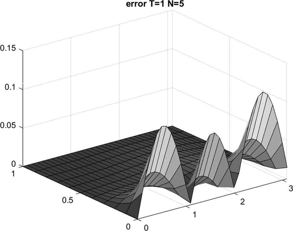
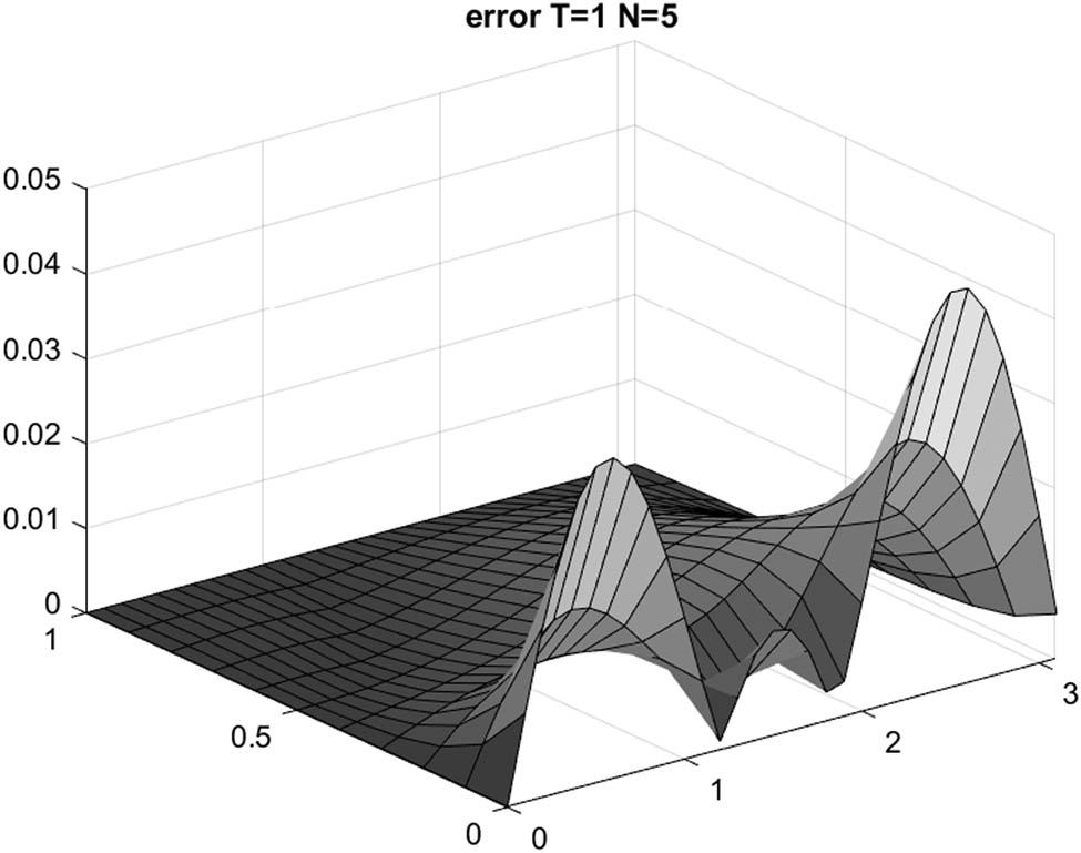
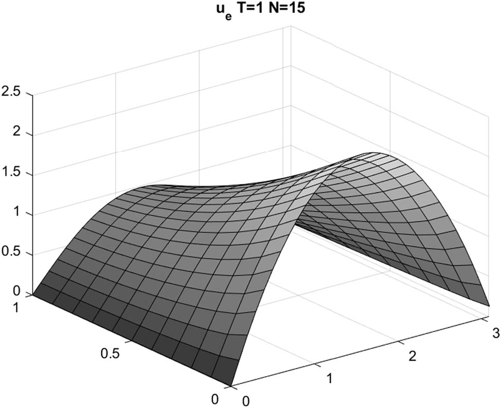
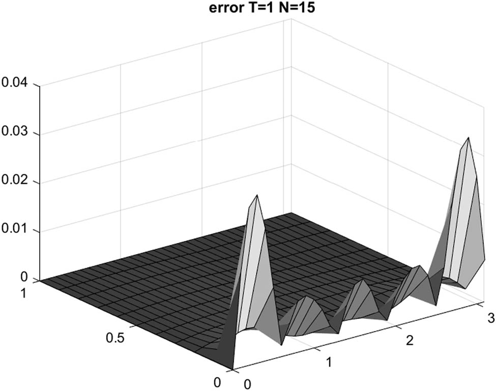
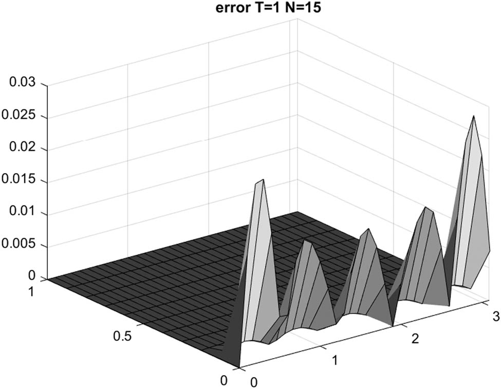
Example 1. We consider an example with f ( x , t ) = t 2 sin 2 x in Eq. (1.1) to demonstrate the accuracy of right proposed scheme. The initial temperature is φ ( x ) = sin x + sin 3 x for 0 ≤ x ≤ π . Then, the exact solution is as follows:

v ( x , t ) = e − t sin x + e − 9 t sin 3 x + F ( x , t ) ,

where

F ( x , t ) = ∫ 0 t e − 4 ( t − τ ) τ 2 d τ sin 2 x = 1 4 t 2 − 1 2 t + 1 8 ( 1 − e − 4 t ) sin 2 x .

Our reconstruction of v ( x , t ) , using the proposed iterative technique is ∑ m = 0 N v m ( x , t ) . Figure 1 shows the exact solution of Example 1. Figures 2, 3, and 4 show the errors for N = 5 with ε = 0.001 , 1 0 − 5 and compare with BPHAM method. Errors in some points for the new scheme and BPHAM method are shown in Tables 1 and 2.

$Figure 1 Example 1: u e {u}_{e} is the exact solution.$

Figure 1

Example 1: u e is the exact solution.

$Figure 2 Example 1: E N {E}_{N} for N = 5 N=5 , T = 1 T=1 , and ε = 0.001 \varepsilon =0.001 .$

Figure 2

Example 1: E N for N = 5 , T = 1 , and ε = 0.001 .

$Figure 3 Example 1: E N {E}_{N} for N = 5 N=5 , T = 1 T=1 , and ε = 1 0 − 5 \varepsilon =1{0}^{-5} .$

Figure 3

Example 1: E N for N = 5 , T = 1 , and ε = 1 0 − 5 .

$Figure 4 Example 1 : E N {E}_{N} for N = 5 N=5 , T = 1 T=1 , and BPHAM method.$

Figure 4

Example 1 : E N for N = 5 , T = 1 , and BPHAM method.

Table 1

E N for v ( x , t ) of Example 1 with N = 5 and T = 1

t	ε = 0.001	ε = 1 0 ‒ 5	BPHAM method
0.95	0.0008493	0.00089405	0.0008945
0.8	0.0035283	0.0036101	0.003616
0.55	0.0082616	0.0083079	0.0083084
0.30	0.016906	0.013106	0.013268
0.05	0.078309	0.032745	0.034288

Table 2

E N for v ( x , t ) of Example 1 with N = 15 and T = 1

t	ε = 0.001	ε = 1 0 ‒ 5	BPHAM method
0.95	0.00011643	1.0443 × 1 0 ‒ 6	8.7353 × 1 0 ‒ 5
0.8	0.00033718	3.6502 × 1 0 ‒ 6	3.5312 × 1 0 ‒ 4
0.55	0.00063062	9.0726 × 1 0 ‒ 6	8.1137 × 1 0 ‒ 5
0.30	0.0039046	5.1504 × 1 0 ‒ 5	1.2957 × 1 0 ‒ 4
0.05	0.045473	0.0005052	3.3484 × 1 0 ‒ 3

Example 2. Suppose φ ( x ) = x ( π − x ) and 0 ≤ x ≤ π . The function has infinite number of Fourier expansion

g ( x ) = 4 π ∑ n = 1 ∞ 4 ( 1 − ( − 1 ) n ) π n 3 sin n x .

Then, the forward problem (1.3) together with Theorem 2.1 yields the noisy inversion input data as follows:

v δ ( x , T ) ≈ 4 π ∑ n = 1 10 4 ( 1 − ( − 1 ) n ) π n 3 e − n 2 T sin n x + F ( x , t ) + δ × randn ( x ) .

We suppose the input data with δ = 0.001 , hence Figure 5 shows the exact solution of Example 2. If we put h = − 0.5 and N = 15 then the experimental results are shown in Figures 6, 7, and 8. The numerical performances of our technique and BPHAM method for N = 5 and N = 15 and errors for ε = 0.001 and ε = 1 0 − 5 and BPHAM method for some points are shown in Tables 3 and 4. Theorem 3.1 confirms the results in the all tables of Examples 1 and 2.

$Figure 5 Example 2: u e {u}_{e} is exact solution.$

Figure 5

Example 2: u e is exact solution.

$Figure 6 Example 2: E N {E}_{N} for N = 15 N=15 , T = 1 T=1 , and ε = 0.001 \varepsilon =0.001 .$

Figure 6

Example 2: E N for N = 15 , T = 1 , and ε = 0.001 .

$Figure 7 Example 2: E N {E}_{N} for N = 15 N=15 , T = 1 T=1 , and ε = 1 0 − 5 \varepsilon =1{0}^{-5} .$

Figure 7

Example 2: E N for N = 15 , T = 1 , and ε = 1 0 − 5 .

$Figure 8 Example 2: E N {E}_{N} for N = 15 N=15 , T = 1 T=1 , and BPHAM method.$

Figure 8

Example 2: E N for N = 15 , T = 1 , and BPHAM method.

Table 3

E N for v ( x , t ) of Example 2 with N = 5 and T = 1

t	ε = 0.001	ε = 1 0 ‒ 5	BPHAM method
0.95	0.0017454	0.0017624	0.0017626
0.8	0.0074165	0.0073405	0.00737
0.55	0.18488	0.018038	0.018034
0.30	0.031817	0.030852	0.30843
0.05	0.045806	0.036219	0.046224

Table 4

E N for v ( x , t ) of Example 2 with N = 15 and T = 1

t	ε = 0.001	ε = 1 0 ‒ 5	BPHAM method
0.95	0.00013386	2.1806 × 1 0 ‒ 6	1.7231 × 1 0 ‒ 4
0.8	0.00041076	8.7021 × 1 0 ‒ 6	7.1973 × 1 0 ‒ 5
0.55	0.000774	2.228 × 1 0 ‒ 5	1.7611 × 1 0 ‒ 4
0.30	0.0011935	4.0121 × 1 0 ‒ 5	3.0125 × 1 0 ‒ 4
0.05	0.0049727	0.000056312	0.00062064

6 Conclusion and remarks

In this article, we proposed a hybrid of numerical schemes for the inverse time problem. This advanced method is equipped with the quasi-reversibility method and after that provides an iterative regularizing strategy for noisy input data that is based on homotopy. This combined method of progress along with mathematical analysis presents important and new theorems regarding error analysis in this field, which achieves very good results compared to other research. Numerical results are also available from this issue. The numerical examples illustrate that using regularization methods can improve the quality of the computed approximate solution. It is also possible to solve the nonlinear inverse equation using the proposed method, but due to the scope and complexity of this research, we will discuss this issue in future works. This article will be a new beginning in the change and evolution of homotopy analysis in inverse problems. Regarding the nonlinearity of the problem, we note that a linearization technique is needed. Because of the long discussion, this issue is being investigated, and the results will be presented in the future. On the other hand, our emphasis is on the one-dimensional problem, and all the analysis of the explained method can be implemented in the two-dimensional mode as well. The convergence of the method is shown pointwise according to the numerical results and Theorem 3.1. But the theory of the optimal error analysis must be improved for this method.

Acknowledgements

The authors would like to thank the two anonymous referees for their very helpful comments, which helped to improve the article.

Funding information: We have no financial resources.
Author contributions: The authors contributed to the design and implementation of the research, analysis of the results, and writing of the manuscript and also they discussed the results and contributed to the final manuscript.
Conflict of interest: There are no competing interests in this article. This research work is not affiliated with any private or military institution, and no material benefits have been received in this study.
Data availability statement: Data are available on request from the authors.

References

[1] Denche M, Bessila K. A modified quasi-boundary value for ill-posed problems. J Math Anal Appl. 2005;301:419–26. 10.1016/j.jmaa.2004.08.001Search in Google Scholar

[2] Huang Y, Zheng Q. Regularization for a class of ill-posed Cauchy problems. Proc Am Math Soc. 2005;133(10):3005–12. 10.1090/S0002-9939-05-07822-6Search in Google Scholar

[3] Huang Y, Quan Z. Regularization for ill-posed Cauchy problems associated with generators of analytic semigroups. J Differ Equ. 2004;203(1):38–54. 10.1016/j.jde.2004.03.035Search in Google Scholar

[4] Dang D, Nguyen HT. Regularization and error estimates for nonhomogeneous backward heat problem. Electr J Differ Equ. 20062006;4:1–10. Search in Google Scholar

[5] Chen Q, Liu JJ. Solving the backward heat conduction problem by data fitting with multiple regularizing parameters. J Comput Math. 2012;30(4):418–32. 10.4208/jcm.1111-m3457Search in Google Scholar

[6] Asl NA, Rostamy D. Identifying an unknown time-dependent boundary source in time-fractional diffusion equation with a non-local boundary condition. J Comput Appl Math. 2019;355:36–50. 10.1016/j.cam.2019.01.018Search in Google Scholar

[7] Mel’nikova IV. Regularization of ill-posed differential problems. Sib Math J. 1992;33:289–98. 10.1007/BF00971100Search in Google Scholar

[8] Lattes R, Lions JL. Method de quasi-reversibility et applications. Paris, France: Dunod; 1967 (English translation Bellman R. New York (NY), USA: Elsevier; 1969). Search in Google Scholar

[9] Miller K. Stabilished quasi-reversibility and other near possible methods for non-well-posed problems. In: Knops RJ, editor. Symposium on Non Well-posed Problems and Logarithmic Convexity, Lecture Notes in Mathematics. Vol. 3. Berlin Heidelberg, Germany: Springer; 1973. p. 161–76. 10.1007/BFb0069627Search in Google Scholar

[10] Qian Z, Fu CL, Shi R. A modified method for a backward heat conduction problem. Appl Math Comput. 2007;185:564–73. 10.1016/j.amc.2006.07.055Search in Google Scholar

[11] Qian Z, Fu CL, Feng XL. A modified method for high order numerical derivatives. Appl Math Comput. 2006;182:1191–200. 10.1016/j.amc.2006.04.059Search in Google Scholar

[12] Qian Z, Fu CL, Xiong XT. A modified for determining the surface heat flux of IHCP. Inverse Prob Sci Eng. 2007;15:249–65. 10.1080/17415970600725128Search in Google Scholar

[13] Yang F, Fu CL. Two regularization methods for identification of the heat source depending only on spatial variable for the heat equation. J Inv Ill-posed Prob. 2009;17:1–16. 10.1515/JIIP.2009.048Search in Google Scholar

[14] Rostamy D, Karimi K. Hypercomplex mathematics and HPM for the time-delayed Burgers equation with convergence analysis. Numer Algorithms. 2011;58:85–101. 10.1007/s11075-011-9448-7Search in Google Scholar

[15] Abbasbandy S. The application of homotopy analysis method to nonlinear equations arising in heat transfer. Phys Lett A. 2006;36:109–13. 10.1016/j.physleta.2006.07.065Search in Google Scholar

[16] Liao SJ. On the homotopy analysis method for nonlinear problems. Appl Math Comput. 2004;147:499–513. 10.1016/S0096-3003(02)00790-7Search in Google Scholar

[17] Park SH, Kim JH. Homotopy analysis method for option pricing under stochastic volatility. Appl Math Lett. 2011;24:1740–4. 10.1016/j.aml.2011.04.034Search in Google Scholar

[18] Liao SJ. Notes on the homotopy analysis method: some definitions and theorems. Commun Nonlinear Sci Numer Simul. 2009;14:983–97. 10.1016/j.cnsns.2008.04.013Search in Google Scholar

[19] Shidfar A, Molabahrami A. A weighted algorithm based on the homotopy analysis method; application to inverse heat conduction problem. Commun Nonlinear Sci Numer Siml. 2010;15:2908–15. 10.1016/j.cnsns.2009.11.011Search in Google Scholar

[20] Watson LT, Haftka RT. Modern homotopy methods in optimization. Comput Methods Appl Mech Eng. 1989;74:289–305. 10.1016/0045-7825(89)90053-4Search in Google Scholar

[21] Rahimi M, Rostamy D. A novel of hybrid regularization on backward piecewise homotopy analysis method for ill-posed problems. J Math. 2023. (in press)Search in Google Scholar

[22] Liu J, Wang B. Solving the backward heat conduction problem by homotopy analysis method. Appl Numer Math. 2018;128:84–97. 10.1016/j.apnum.2018.02.002Search in Google Scholar

[23] Liao SJ. Beyond perturbation. Introduction to the homotopy analysis method. Boca Raton (FL), USA: Chapman Hall/CRC Press; 2003. Search in Google Scholar

[24] Murio DA. Mollification and space marching. In: Woodburg K, editor. Inverse engineering handbook. Boca Raton (FL), USA: CRC Press, 2002. 10.1201/9781420041613.ch4Search in Google Scholar

[25] Bodaghi S, Zakeri A, Amiraslani A. A numerical scheme based on discrete mollification method using Bernstein basis polynomials for solving the inverse one-dimensional Stefan problem. Inverse Problems Sci Eng. 2020;28(11):1528–50. 10.1080/17415977.2020.1733996Search in Google Scholar

[26] Coles C, Murio DA. Identification of parameters in the 2-D IHCP. Comput Math Appl. 2000;40:939–56. 10.1016/S0898-1221(00)85005-1Search in Google Scholar

Received: 2023-01-30

Revised: 2023-05-21

Accepted: 2023-06-18

Published Online: 2023-07-27

This work is licensed under the Creative Commons Attribution 4.0 International License.

Articles in the same Issue

https://doi.org/10.1515/nleng-2022-0304

Keywords for this article

heat conduction; backward conduction; ill-posed problem; homotopy analysis method; quasi-reversibility; discrete mollification

Creative Commons

BY 4.0