An iterative approach using Sawi transform for fractional telegraph equation in diversified dimensions
-
Mamta Kapoor
 and
Samanyu Khosla
and
Samanyu Khosla

Abstract
In the present study, 1D, 2D, and 3D fractional hyperbolic telegraph equations in Caputo sense have been solved using an iterative method using Sawi transform. These equations serve as a model for signal analysis of electrical impulse transmission and propagation. Along with a table of Sawi transform of some popular functions, some helpful results on Sawi transform are provided. To demonstrate the effectiveness of the suggested method, five examples in 1D, one example in 2D, and one example in 3D are solved using the proposed scheme. Error analysis comparing approximate and exact solutions using graphs and tables has been provided. The proposed scheme is robust, effective, and easy to implement and can be implemented on variety of fractional partial differential equations to obtain precise series approximations.
1 Introduction
Fractional calculus deals with derivatives of fractional orders, and the concept can be dated back to a letter from Leibnitz to L’Hospital discussing the possibility of fractional order derivatives [1]. In the present day, multiple different fractional derivatives exist, for example Caputo derivative, Riemann–Liouville derivative [2], Atangana–Baleanu Caputo derivative [3], etc. There exists a wide variety of fractional partial differential equations (FPDEs), one such type of equation being the fractional hyperbolic telegraph equation, which is used as a model in signal analyses of transmission and propagation of electrical impulses and other fields [4]. Many methods have been developed and used to solve FPDEs, such as iterative Laplace transform method [5], homotopy analysis method [6], finite difference method [7], Adomian decomposition method and variational iteration method [8], computational model based on hybrid B-spline collocation method [9], etc.
In the 1880s, Oliver Heaviside developed the telegraph equation to describe the time and distance on an electric transmission line with current and voltage [10]. As fractional hyperbolic telegraph equations (FHTEs) are a kind of FPDE, it is difficult to solve them by the usual means. Therefore, multiple techniques have been developed and applied to solve FHTEs, such as Chebyshev Tau method [11], Sinc Legendre collocation method [12], He’s variational iteration Method [13], fractional skewed grid Crank–Nicolson scheme [14], meshless method using radial basis function [15], hybrid meshless method by combining GFDM in space domain and Houbolt method in temporal dimension [16], shifted Jacobi collocation scheme [17], finite difference scheme based on extended cubic-B spline method [18], least square homotopy perturbation technique [19], etc.
Definition 1
One, two, and three dimensional (1D, 2D, and 3D) FHTEs are given as follows [20]:
where
Different transforms like Natural transform [21], Sumudu transform [22], Mohand transform [23] etc., can be applied on pre-existing techniques to solve FPDEs, for example, Natural transform has been used with Adomian decomposition method, also known as Natural transform decomposition method to solve FHTEs [24], Shehu Transform is used in an analytical approach to solve time-fractional Schrödinger equations [25], differential transform method has been used to solve FPDEs like Bagley–Torvik equation and composite fractional oscillation equation [26], a method developed by combining time discretization and Laplace transform method has been used to numerically solve fractional differential equations via quadrature rule [27], Sumudu transform has been combined with homotopy perturbation method to solve non-linear fractional differential equations [28], inverse fractional Shehu transform method has been used to solve fractional differential equations [29] etc. In the present study, Sawi transform is used in an iterative approach, which is based on an analytical approach using Shehu transform to solve FHTEs [20], to obtain a series solution to FHTEs in 1D, 2D, and 3D.
Definition 2
Sawi transform of a function
where
Definition 3
Linearity property of Sawi transform is as follows [30]:
Definition 4
Scaling property of Sawi transform is as follows [30]:
Then,
Let
Definition 5
Translation property of Sawi transform is as follows [30]:
Then,
Definition 6
Caputo derivative of a function
where
Definition 7
Sawi transform of Caputo derivative of a function
2 Outline of the study
Outline of the study has been provided below.
In Section 3, general formula for the
In Section 4, a total of seven examples have been solved to illustrate the efficacy of the proposed method. Examples 1, 4, and 5 involve
In Section 5, graphs and tables for Examples 1, 2, 4, 5, 6, and 7 have been provided to perform error analysis.
In Section 6, the conclusion has been provided.
3 Development of the formula
The form of
where
Now, linear and nonlinear operators can be decomposed in the following manner:
The general formulae for 2D and 3D can also be derived in a similar manner. Their proofs have been provided in Appendixes A and B, respectively. It can be observed that the first term
4 Examples and calculations
Each example has a series solution calculated at a specific
where
Applying Sawi transform on Eq. (10)
Considering
Using Eq. (12)
Using Eq. (12)
Using Eq. (12)
Putting
Also, the fractional equation becomes,
Given the same initial conditions, the exact solution of this differential equation is
Example 2
Consider the following 2D time FHTE [20]:
where
Applying Sawi transform on Eq. (13)
Considering
Using Eq. (15)
Using Eq. (15)
Using Eq. (15)
Putting
Also, the fractional equation becomes
Given the same initial conditions, the exact solution of this differential equation is
Example 3
Consider the following 3D time FHTE [20]
where
Applying Sawi transform on Eq. (16)
Considering
Using Eq. (18)
Using Eq. (18)
Using Eq. (18)
Putting
where
Applying Sawi transform on Eq. (19)
Considering
Using Eq. (21)
Using Eq. (21)
Using Eq. (21)
Putting
Also, the fractional equation becomes
Given the same initial conditions, the exact solution of this differential equation is
where
Applying Sawi transform on Eq. (22)
Considering
Using Eq. (24)
Using Eq. (24)
Using Eq. (24)
Putting
Also, the fractional equation becomes
Given the same initial conditions, the exact solution of this differential equation is
where
Applying Sawi transform on Eq. (25)
Considering
Using Eq. (27)
Using Eq. (27)
Using Eq. (27)
Putting
Also, the fractional equation becomes
Given the same initial conditions, the exact solution of this differential equation is
where
Applying Sawi transform on Eq. (28)
Considering
Using Eq. (30)
Using Eq. (31)
Using Eq. (31)
Putting
Also, the fractional equation becomes
Given the same initial conditions, the exact solution of this differential equation is
Exact and approximate solutions of Examples 1, 4 and 5 are compared for
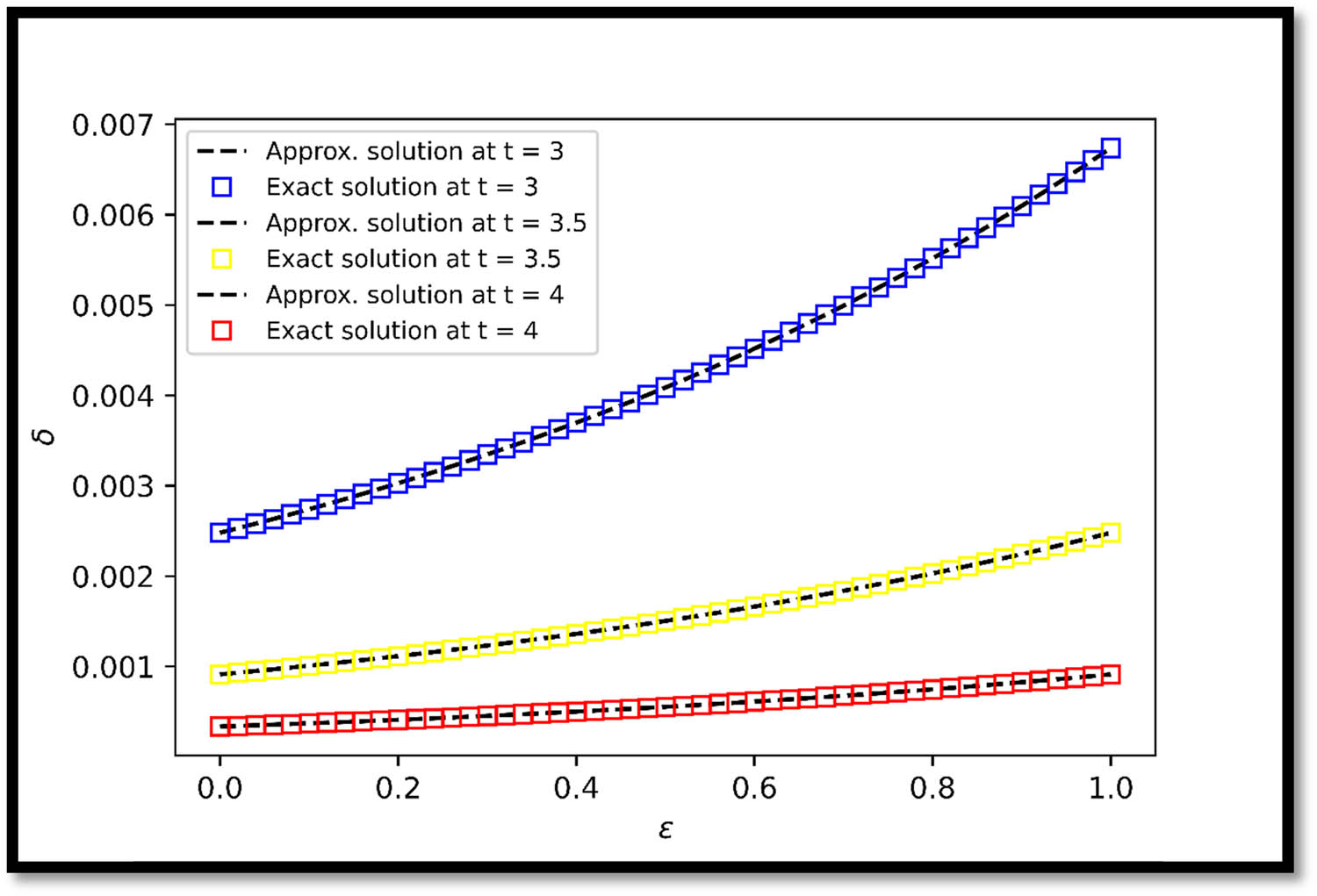
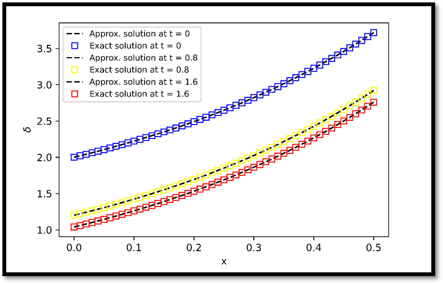
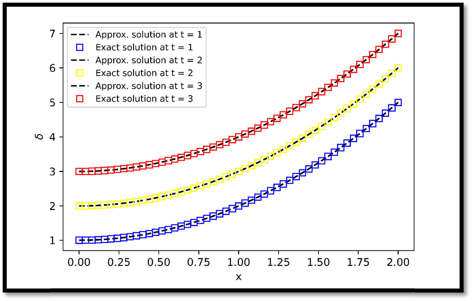
Comparing exact and approximate solutions of Example 1 at
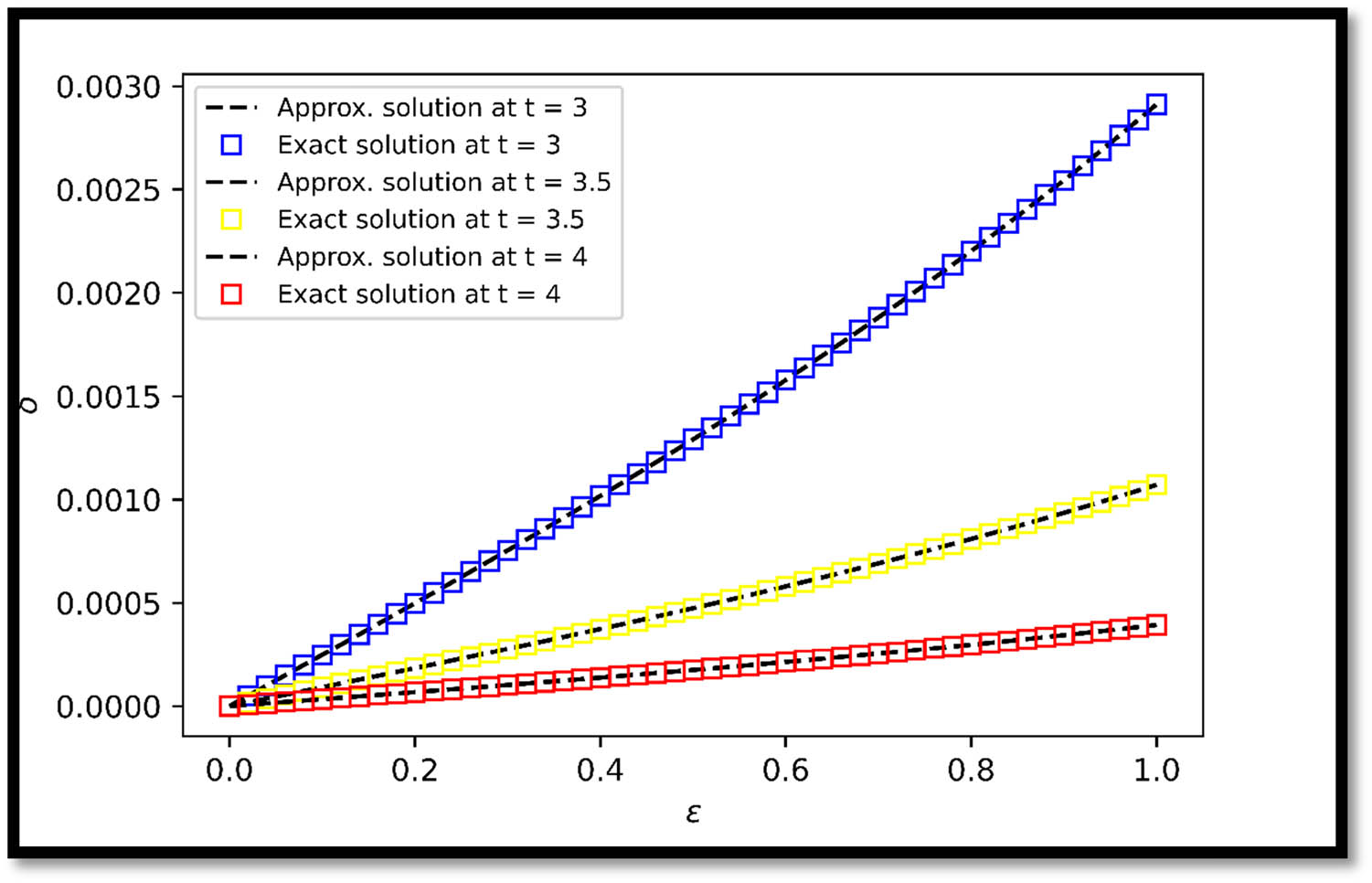
Comparing exact and approximate solutions of Example 4 at
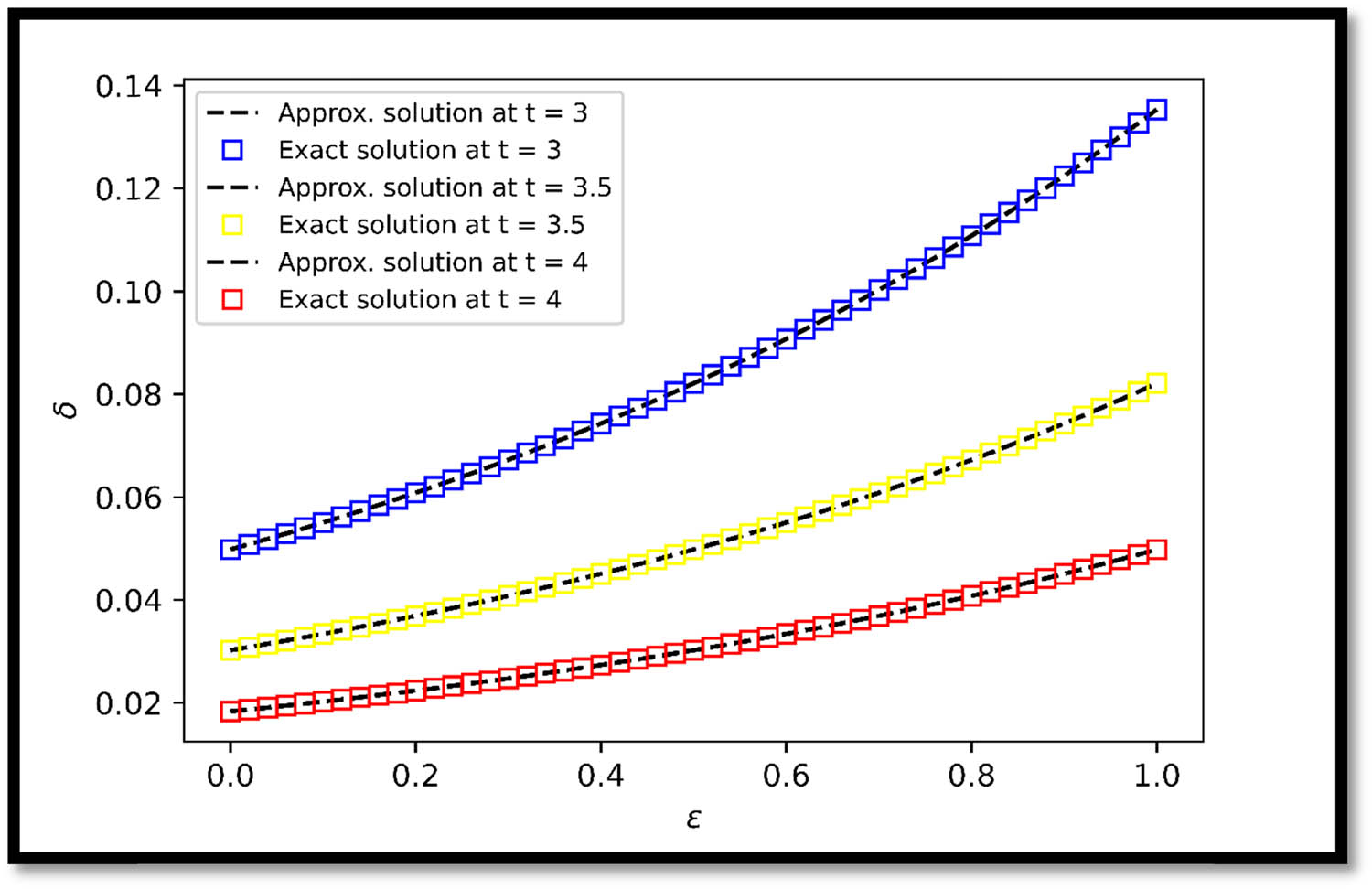
Comparing exact and approximate solutions of Example 5 at
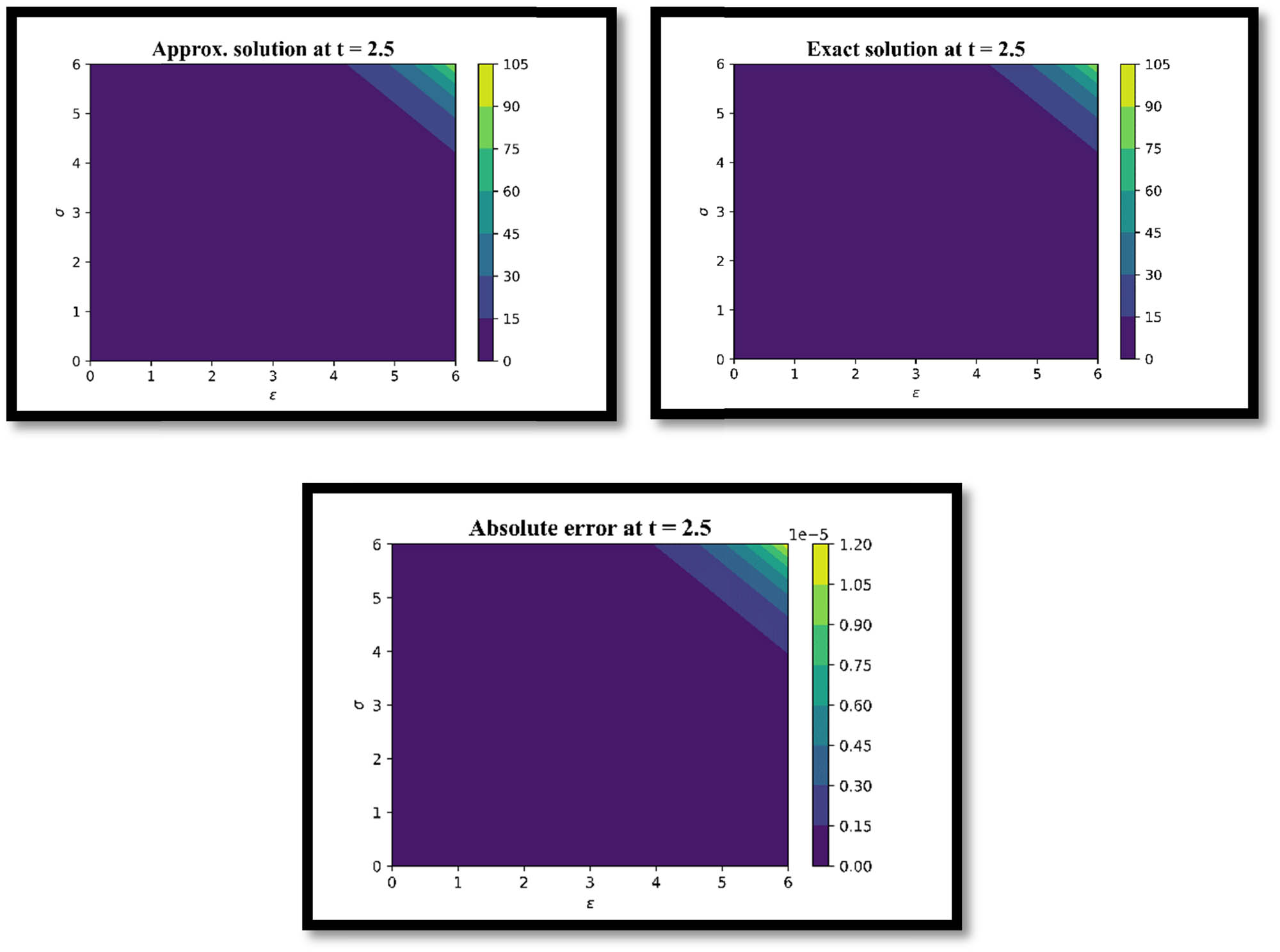
Comparing exact and approximate solutions of Example 2 at
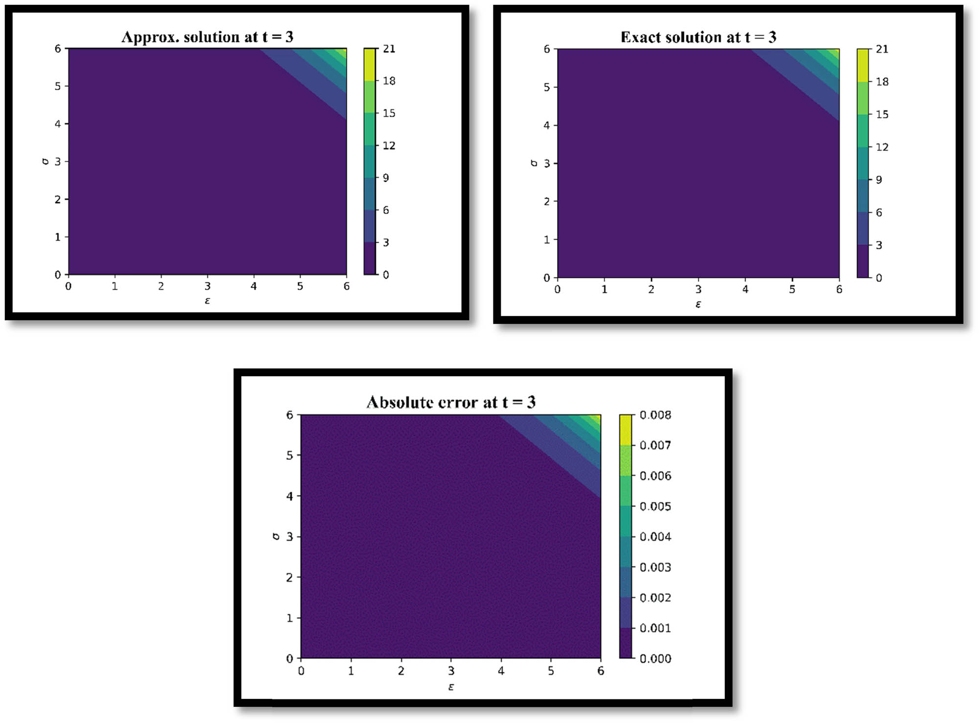
Comparing exact and approximate solutions of Example 2 at
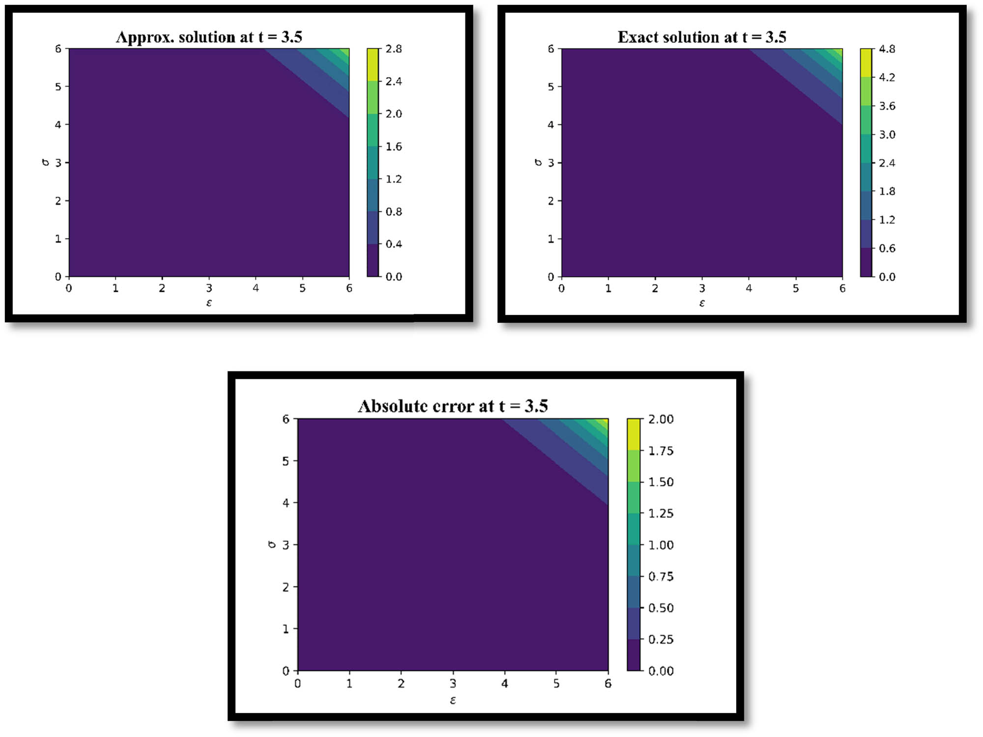
Comparing exact and approximate solutions of Example 2 at
Comparing exact and approximate solutions of Example 6 at
Comparing exact and approximate solutions of Example 7 at
Sawi transform of common functions [33]
|
|
|
|
|---|---|---|
| 1 |
|
|
| 2 |
|
1 |
| 3 |
|
|
| 4 |
|
|
| 5 |
|
|
| 6 |
|
|
| 7 |
|
|
| 8 |
|
|
Inverse Sawi transform of common functions [33]
|
|
|
|
|---|---|---|
| 1 |
|
|
| 2 | 1 |
|
| 3 |
|
|
| 4 |
|
|
| 5 |
|
|
| 6 |
|
|
| 7 |
|
|
| 8 |
|
|
For consistency, the number of equally spaced values for
Error analysis for Example 1
|
|
Exact value at
|
Approx. value at
|
|
Exact value at
|
Approx. value at
|
|
Exact value at
|
Approx. value at
|
|
|---|---|---|---|---|---|---|---|---|---|
| 10 | 0.367879 | 0.367999 | 0.000119 | 0.049787 | 0.262911 | 0.213124 | 0.006738 | 16.32522 | 16.31849 |
| 20 | 0.367879 | 0.367879 | 1.02 × 10⁻¹³ | 0.049787 | 0.049787 | 1.98 × 10⁻⁷ | 0.006738 | 0.007653 | 0.000915 |
| 30 | 0.29523 | 0.29523 | 1.28 × 10⁻¹⁵ | 0.033373 | 0.033373 | 4.55 × 10⁻¹⁵ | 0.006738 | 0.006738 | 3.69 × 10⁻¹⁰ |
| ↓ Up to
|
↓ Up to
|
↓ Up to
|
Error analysis for Example 2
|
|
Exact value at
|
Approx. value at
|
|
Exact value at
|
Approx. value at
|
|
Exact value at
|
Approx. value at
|
|
|---|---|---|---|---|---|---|---|---|---|
| 10 | 49020.8 | 49020.83 | 0.027523 | 36315.5 | 36315.82 | 0.313187 | 26903.19 | 26905.46 | 2.275563 |
| 15 | 49020.8 | 49020.8 | 1.34 × 10⁻⁷ | 36315.5 | 36315.5 | 4.69 × 10⁻⁶ | 26903.19 | 26903.19 | 8.54 × 10⁻⁵ |
| 20 | 49020.8 | 49020.8 | 6.55 × 10⁻¹¹ | 12088.38 | 12088.38 | 2.91 × 10⁻¹¹ | 26903.19 | 26903.19 | 7.13 × 10⁻¹⁰ |
| ↓ Up to
|
↓ Up to
|
↓ Up to
|
Error analysis for Example 4
|
|
Exact value at
|
Approx. value at
|
|
Exact value at
|
Approx. value at
|
|
Exact value at
|
Approx. value at
|
|
|---|---|---|---|---|---|---|---|---|---|
| 10 | 0.159046 | 0.159098 | 5.16 × 10⁻⁵ | 0.021525 | 0.113665 | 0.09214 | 0.002913 | 7.057923 | 7.05501 |
| 20 | 0.159046 | 0.159046 | 4.41 × 10⁻¹⁴ | 0.021525 | 0.021525 | 8.55 × 10⁻⁸ | 0.002913 | 0.003309 | 0.000396 |
| 30 | 0.146795 | 0.146795 | 8.05 × 10⁻¹⁶ | 0.017259 | 0.017259 | 1.6 × 10⁻¹⁵ | 0.002913 | 0.002913 | 1.6 × 10⁻¹⁰ |
| ↓ Up to
|
↓ Up to
|
↓ Up to
|
Error analysis for Example 5
|
|
Exact value at
|
Approx. value at
|
|
Exact value at
|
Approx. value at
|
|
Exact value at
|
Approx. value at
|
|
|---|---|---|---|---|---|---|---|---|---|
| 10 | 1 | 1 | 6.28 × 10⁻⁸ | 0.367879 | 0.367999 | 0.000119 | 0.135335 | 0.144955 | 0.00962 |
| 20 | 0.398519 | 0.398519 | 2.22 × 10⁻¹⁶ | 0.367879 | 0.367879 | 1.02 × 10⁻¹³ | 0.135335 | 0.135335 | 4.89 × 10⁻¹⁰ |
| 30 | 0.398519 | 0.398519 | 2.22 × 10⁻¹⁶ | 0.29523 | 0.29523 | 1.28 × 10⁻¹⁵ | 0.132655 | 0.132655 | 4.44 × 10⁻¹⁵ |
| ↓ Up to
|
↓ Up to
|
↓ Up to
|
Error analysis for Example 6
|
|
Exact value at
|
Approx. value at
|
|
Exact value at
|
Approx. value at
|
|
Exact value at
|
Approx. value at
|
|
|---|---|---|---|---|---|---|---|---|---|
| 4 | 2.853617 | 2.853589 | 2.79 × 10⁻⁵ | 2.736597 | 2.73657 | 2.79 × 10⁻⁵ | 2.720761 | 2.720733 | 2.79 × 10⁻⁵ |
| 7 | 2.853617 | 2.853617 | 1.23 × 10⁻¹¹ | 2.736597 | 2.736597 | 1.23 × 10⁻¹¹ | 2.720761 | 2.720761 | 1.23 × 10⁻¹¹ |
| 10 | 1.957454 | 1.957454 | 4.44 × 10⁻¹⁶ | 2.527606 | 2.527606 | 4.44 × 10⁻¹⁶ | 2.098414 | 2.098414 | 4.44 × 10⁻¹⁶ |
| ↓ Up to
|
↓ Up to
|
↓ Up to
|
Error Analysis for Example 7
|
|
Exact value at
|
Approx. value at
|
|
Exact value at
|
Approx value at
|
|
Exact value at
|
Approx. value at
|
|
|---|---|---|---|---|---|---|---|---|---|
| 4 | 5 | 4.987302 | 0.012698 | 6 | 5.987302 | 0.012698 | 7 | 6.987302 | 0.012698 |
| 7 | 5 | 5 | 3.76 × 10⁻⁷ | 6 | 6 | 3.76 × 10⁻⁷ | 7 | 7 | 3.76 × 10⁻⁷ |
| 10 | 5 | 5 | 8.62 × 10⁻¹³ | 6 | 6 | 8.62 × 10⁻¹³ | 7 | 7 | 8.62 × 10⁻¹³ |
| ↓ Up to
|
↓ Up to
|
↓ Up to
|
5 Conclusion
In the present study, an iterative scheme was proposed involving the Sawi transform for solving FHTEs. A general formula for the proposed method was developed for
-
Funding information: Not available.
-
Author contributions: Conceptualization: M.K.; programming: S.K.; drafting: S.K.; calculation: M.K. and S.K.
-
Conflict of interest: Not applicable.
Appendix A
The form of
where
Now,
Appendix B
The form of
where
Now,
References
[1] Leibniz GW. Letter from Hanover, Germany, September 30, 1695 to G.F.A L’Hospital. Mathematische Schriften. 1849;2:301–2.Search in Google Scholar
[2] Li C, Qian D, Chen Y. On Riemann-Liouville and Caputo derivatives. Discret Dyn Nat Soc. 2011;2011.10.1155/2011/562494Search in Google Scholar
[3] Yadav S, Pandey RK, Shukla AK. Numerical approximations of Atangana–Baleanu Caputo derivative and its application. Chaos Solitons Fractals. 2019;118:58–64.10.1016/j.chaos.2018.11.009Search in Google Scholar
[4] Okubo A. Application of the telegraph equation to oceanic diffusion: Another mathematic model. Technical Report 69. Chesapeake Bay Institute, The Johns Hopkins University; 1971.Search in Google Scholar
[5] Jafari H, Nazari M, Baleanu D, Khalique CM. A new approach for solving a system of fractional partial differential equations. Comput Math Appl. 2013;66(5):838–43.10.1016/j.camwa.2012.11.014Search in Google Scholar
[6] Dehghan M, Manafian J, Saadatmandi A. Solving nonlinear fractional partial differential equations using the homotopy analysis method. Numer Methods Partial Differ Equ An Int J. 2010;26(2):448–79.10.1002/num.20460Search in Google Scholar
[7] Zhang Y. A finite difference method for fractional partial differential equation. Appl Math Comput. 2009;215(2):524–9.10.1016/j.amc.2009.05.018Search in Google Scholar
[8] Momani S, Odibat Z. Analytical approach to linear fractional partial differential equations arising in fluid mechanics. Phys Lett A. 2006;355(4–5):271–9.10.1016/j.physleta.2006.02.048Search in Google Scholar
[9] Singh J, Kumar D, Purohit SD, Mishra AM, Bohra M. An efficient numerical approach for fractional multidimensional diffusion equations with exponential memory. Numer Methods Partial Differ Equ. 2021;37(2):1631–51.10.1002/num.22601Search in Google Scholar
[10] Khan H, Shah R, Kumam P, Baleanu D, Arif M. An efficient analytical technique, for the solution of fractional-order telegraph equations. Mathematics. 2019;7(5):426.10.3390/math7050426Search in Google Scholar
[11] Saadatmandi A, Dehghan M. Numerical solution of hyperbolic telegraph equation using the Chebyshev Tau method. Numer Methods Partial Differ Equ An Int J. 2010;26(1):239–52.10.1002/num.20442Search in Google Scholar
[12] Sweilam NH, Nagy AM, El-Sayed AA. Solving time-fractional order telegraph equation via Sinc–Legendre collocation method. Mediterr J Math. 2016;13:5119–33.10.1007/s00009-016-0796-3Search in Google Scholar
[13] Sevimlican A. An approximation to solution of space and time fractional telegraph equations by He’s variational iteration method. Math Probl Eng. 2010;2010:290631.10.1155/2010/290631Search in Google Scholar
[14] Ali A, Ali NH. On skewed grid point iterative method for solving 2D hyperbolic telegraph fractional differential equation. Adv Differ Equ. 2019;2019(1):1–29.10.1186/s13662-019-2238-6Search in Google Scholar
[15] Hosseini VR, Chen W, Avazzadeh Z. Numerical solution of fractional telegraph equation by using radial basis functions. Eng Anal Bound Elem. 2014;38:31–9.10.1016/j.enganabound.2013.10.009Search in Google Scholar
[16] Zhou Y, Qu W, Gu Y, Gao H. A hybrid meshless method for the solution of the second order hyperbolic telegraph equation in two space dimensions. Eng Anal Bound Elem. 2020;115:21–7.10.1016/j.enganabound.2020.02.015Search in Google Scholar
[17] Hafez RM, Youssri YH. Shifted Jacobi collocation scheme for multidimensional time-fractional order telegraph equation. Iran J Numer Anal Optim. 2020;10(1):195–223.Search in Google Scholar
[18] Akram T, Abbas M, Ismail AI, Ali NH, Baleanu D. Extended cubic B-splines in the numerical solution of time fractional telegraph equation. Adv Differ Equ. 2019;2019(1):1–20.10.1186/s13662-019-2296-9Search in Google Scholar
[19] Kumar R, Koundal R, Shehzad SA. Least square homotopy solution to hyperbolic telegraph equations: Multi-dimension analysis. Int J Appl Comput Math. 2020;6:1–9.10.1007/s40819-019-0763-3Search in Google Scholar
[20] Kapoor M, Shah NA, Saleem S, Weera W. An analytical approach for fractional hyperbolic telegraph equation using Shehu transform in one, two and three dimensions. Mathematics. 2022;10(12):1961.10.3390/math10121961Search in Google Scholar
[21] Khan ZH, Khan WA. N-transform-properties and applications. NUST J Eng Sci. 2008;1(1):127–33.Search in Google Scholar
[22] Watugala G. Sumudu transform: A new integral transform to solve differential equations and control engineering problems. Integr Educ. 1993;24(1):35–43.10.1080/0020739930240105Search in Google Scholar
[23] Qureshi S, Yusuf A, Aziz S. On the use of Mohand integral transform for solving fractional-order classical Caputo differential equations. J Appl Math Comput Mech. 2020;19(3):99–109.10.17512/jamcm.2020.3.08Search in Google Scholar
[24] Khan H, Shah R, Baleanu D, Kumam P, Arif M. Analytical solution of fractional-order hyperbolic telegraph equation, using natural transform decomposition method. Electronics. 2019;8(9):1015.10.3390/electronics8091015Search in Google Scholar
[25] Kapoor M. Shehu transform on time-fractional Schrödinger equations–an analytical approach. Int J Nonlinear Sci Numer Simul. 2022.10.1515/ijnsns-2021-0423Search in Google Scholar
[26] Arikoglu A, Ozkol I. Solution of fractional differential equations by using differential transform method. Chaos Solitons Fractals. 2007;34(5):1473–81.10.1016/j.chaos.2006.09.004Search in Google Scholar
[27] Soradi-Zeid S, Mesrizadeh M, Cattani C. Numerical solutions of fractional differential equations by using Laplace transformation method and quadrature rule. Fractal Fract. 2021;5(3):111.10.3390/fractalfract5030111Search in Google Scholar
[28] Yousif EA, Hamed SH. Solution of nonlinear fractional differential equations using the homotopy perturbation Sumudu transform method. Appl Math Sci. 2014;8(44):2195–210.10.12988/ams.2014.4285Search in Google Scholar
[29] Khalouta A, Kadem A. A new method to solve fractional differential equations: Inverse fractional Shehu transform method. Appl Appl Math Int J (AAM). 2019;14(2):19.10.17512/jamcm.2020.3.04Search in Google Scholar
[30] Higazy M, Aggarwal S. Sawi transformation for system of ordinary differential equations with application. Ain Shams Eng J. 2021;12(3):3173–82.10.1016/j.asej.2021.01.027Search in Google Scholar
[31] Srivastava VK, Awasthi MK, Tamsir M. RDTM solution of Caputo time fractional-order hyperbolic telegraph equation. AIP Adv. 2013;3(3):032142.10.1063/1.4799548Search in Google Scholar
[32] Hussein MA. A review on integral transforms of fractional integral and derivative. Int Acad J Sci Eng. 2022;9:52–6.10.9756/IAJSE/V9I2/IAJSE0914Search in Google Scholar
[33] Aggarwal S, Gupta AR. Dualities between some useful integral transforms and Sawi transform. Int J Recent Technol Eng. 2019;8(3):5978–82.10.35940/ijrte.C5870.098319Search in Google Scholar
[34] Prakash A. Analytical method for space-fractional telegraph equation by homotopy perturbation transform method. Nonlinear Eng. 2016;5(2):123–8.10.1515/nleng-2016-0008Search in Google Scholar
[35] Prakash A, Kumar M. Numerical method for space-and time-fractional telegraph equation with generalized Lagrange multipliers. Prog Fract Differ Appl. 2019;5(2):111–23.10.18576/pfda/050203Search in Google Scholar
© 2023 the author(s), published by De Gruyter
This work is licensed under the Creative Commons Attribution 4.0 International License.
Articles in the same Issue
- Research Articles
- The regularization of spectral methods for hyperbolic Volterra integrodifferential equations with fractional power elliptic operator
- Analytical and numerical study for the generalized q-deformed sinh-Gordon equation
- Dynamics and attitude control of space-based synthetic aperture radar
- A new optimal multistep optimal homotopy asymptotic method to solve nonlinear system of two biological species
- Dynamical aspects of transient electro-osmotic flow of Burgers' fluid with zeta potential in cylindrical tube
- Self-optimization examination system based on improved particle swarm optimization
- Overlapping grid SQLM for third-grade modified nanofluid flow deformed by porous stretchable/shrinkable Riga plate
- Research on indoor localization algorithm based on time unsynchronization
- Performance evaluation and optimization of fixture adapter for oil drilling top drives
- Nonlinear adaptive sliding mode control with application to quadcopters
- Numerical simulation of Burgers’ equations via quartic HB-spline DQM
- Bond performance between recycled concrete and steel bar after high temperature
- Deformable Laplace transform and its applications
- A comparative study for the numerical approximation of 1D and 2D hyperbolic telegraph equations with UAT and UAH tension B-spline DQM
- Numerical approximations of CNLS equations via UAH tension B-spline DQM
- Nonlinear numerical simulation of bond performance between recycled concrete and corroded steel bars
- An iterative approach using Sawi transform for fractional telegraph equation in diversified dimensions
- Investigation of magnetized convection for second-grade nanofluids via Prabhakar differentiation
- Influence of the blade size on the dynamic characteristic damage identification of wind turbine blades
- Cilia and electroosmosis induced double diffusive transport of hybrid nanofluids through microchannel and entropy analysis
- Semi-analytical approximation of time-fractional telegraph equation via natural transform in Caputo derivative
- Analytical solutions of fractional couple stress fluid flow for an engineering problem
- Simulations of fractional time-derivative against proportional time-delay for solving and investigating the generalized perturbed-KdV equation
- Pricing weather derivatives in an uncertain environment
- Variational principles for a double Rayleigh beam system undergoing vibrations and connected by a nonlinear Winkler–Pasternak elastic layer
- Novel soliton structures of truncated M-fractional (4+1)-dim Fokas wave model
- Safety decision analysis of collapse accident based on “accident tree–analytic hierarchy process”
- Derivation of septic B-spline function in n-dimensional to solve n-dimensional partial differential equations
- Development of a gray box system identification model to estimate the parameters affecting traffic accidents
- Homotopy analysis method for discrete quasi-reversibility mollification method of nonhomogeneous backward heat conduction problem
- New kink-periodic and convex–concave-periodic solutions to the modified regularized long wave equation by means of modified rational trigonometric–hyperbolic functions
- Explicit Chebyshev Petrov–Galerkin scheme for time-fractional fourth-order uniform Euler–Bernoulli pinned–pinned beam equation
- NASA DART mission: A preliminary mathematical dynamical model and its nonlinear circuit emulation
- Nonlinear dynamic responses of ballasted railway tracks using concrete sleepers incorporated with reinforced fibres and pre-treated crumb rubber
- Two-component excitation governance of giant wave clusters with the partially nonlocal nonlinearity
- Bifurcation analysis and control of the valve-controlled hydraulic cylinder system
- Engineering fault intelligent monitoring system based on Internet of Things and GIS
- Traveling wave solutions of the generalized scale-invariant analog of the KdV equation by tanh–coth method
- Electric vehicle wireless charging system for the foreign object detection with the inducted coil with magnetic field variation
- Dynamical structures of wave front to the fractional generalized equal width-Burgers model via two analytic schemes: Effects of parameters and fractionality
- Theoretical and numerical analysis of nonlinear Boussinesq equation under fractal fractional derivative
- Research on the artificial control method of the gas nuclei spectrum in the small-scale experimental pool under atmospheric pressure
- Mathematical analysis of the transmission dynamics of viral infection with effective control policies via fractional derivative
- On duality principles and related convex dual formulations suitable for local and global non-convex variational optimization
- Study on the breaking characteristics of glass-like brittle materials
- The construction and development of economic education model in universities based on the spatial Durbin model
- Homoclinic breather, periodic wave, lump solution, and M-shaped rational solutions for cold bosonic atoms in a zig-zag optical lattice
- Fractional insights into Zika virus transmission: Exploring preventive measures from a dynamical perspective
- Rapid Communication
- Influence of joint flexibility on buckling analysis of free–free beams
- Special Issue: Recent trends and emergence of technology in nonlinear engineering and its applications - Part II
- Research on optimization of crane fault predictive control system based on data mining
- Nonlinear computer image scene and target information extraction based on big data technology
- Nonlinear analysis and processing of software development data under Internet of things monitoring system
- Nonlinear remote monitoring system of manipulator based on network communication technology
- Nonlinear bridge deflection monitoring and prediction system based on network communication
- Cross-modal multi-label image classification modeling and recognition based on nonlinear
- Application of nonlinear clustering optimization algorithm in web data mining of cloud computing
- Optimization of information acquisition security of broadband carrier communication based on linear equation
- A review of tiger conservation studies using nonlinear trajectory: A telemetry data approach
- Multiwireless sensors for electrical measurement based on nonlinear improved data fusion algorithm
- Realization of optimization design of electromechanical integration PLC program system based on 3D model
- Research on nonlinear tracking and evaluation of sports 3D vision action
- Analysis of bridge vibration response for identification of bridge damage using BP neural network
- Numerical analysis of vibration response of elastic tube bundle of heat exchanger based on fluid structure coupling analysis
- Establishment of nonlinear network security situational awareness model based on random forest under the background of big data
- Research and implementation of non-linear management and monitoring system for classified information network
- Study of time-fractional delayed differential equations via new integral transform-based variation iteration technique
- Exhaustive study on post effect processing of 3D image based on nonlinear digital watermarking algorithm
- A versatile dynamic noise control framework based on computer simulation and modeling
- A novel hybrid ensemble convolutional neural network for face recognition by optimizing hyperparameters
- Numerical analysis of uneven settlement of highway subgrade based on nonlinear algorithm
- Experimental design and data analysis and optimization of mechanical condition diagnosis for transformer sets
- Special Issue: Reliable and Robust Fuzzy Logic Control System for Industry 4.0
- Framework for identifying network attacks through packet inspection using machine learning
- Convolutional neural network for UAV image processing and navigation in tree plantations based on deep learning
- Analysis of multimedia technology and mobile learning in English teaching in colleges and universities
- A deep learning-based mathematical modeling strategy for classifying musical genres in musical industry
- An effective framework to improve the managerial activities in global software development
- Simulation of three-dimensional temperature field in high-frequency welding based on nonlinear finite element method
- Multi-objective optimization model of transmission error of nonlinear dynamic load of double helical gears
- Fault diagnosis of electrical equipment based on virtual simulation technology
- Application of fractional-order nonlinear equations in coordinated control of multi-agent systems
- Research on railroad locomotive driving safety assistance technology based on electromechanical coupling analysis
- Risk assessment of computer network information using a proposed approach: Fuzzy hierarchical reasoning model based on scientific inversion parallel programming
- Special Issue: Dynamic Engineering and Control Methods for the Nonlinear Systems - Part I
- The application of iterative hard threshold algorithm based on nonlinear optimal compression sensing and electronic information technology in the field of automatic control
- Equilibrium stability of dynamic duopoly Cournot game under heterogeneous strategies, asymmetric information, and one-way R&D spillovers
- Mathematical prediction model construction of network packet loss rate and nonlinear mapping user experience under the Internet of Things
- Target recognition and detection system based on sensor and nonlinear machine vision fusion
- Risk analysis of bridge ship collision based on AIS data model and nonlinear finite element
- Video face target detection and tracking algorithm based on nonlinear sequence Monte Carlo filtering technique
- Adaptive fuzzy extended state observer for a class of nonlinear systems with output constraint