
Dynamic analysis of particulate pollution in haze in Harbin city, Northeast China
-
Lei Wang
 ,
Jiarong Deng
,
Jiarong Deng

Abstract
Based on the air quality data of Harbin in winter from 2015 to 2017, the national winter straw combustion data from 2016 to 2017 and the mixed single particle Lagrange comprehensive track model, Hybrid Single-Particle Lagrangian Integrated Trajectory Model (HYSPLIT), dynamic analysis of Harbin’s winter air quality status and influencing factors. The air quality data were analyzed; it was found that the main pollutants in winter in Harbin were SO2, NO2, PM10 (particles with aerodynamic diameter ≤10 µm), and PM2.5 (particles with aerodynamic diameter ≤2.5 µm); the annual air pollution situation deteriorated sharply from November and continued until March of the following year. Through the research on straw fire prevention points in Harbin, the spatial pattern characteristics and causes of persistent haze in Harbin from 2015 to 2017 were dynamically analyzed. Combining the backward trajectory model to trace the source and trend of air mass in pollution, it is found that the air mass trend is consistent with the distribution of straw-burning points. The research results show that (1) during the winter from 2015 to 2017, the overall air quality situation in Harbin improved, the number of serious pollution days decreased year by year, and the main atmospheric pollutants were PM10 and PM2.5. In October and November, the pollution concentration peaked, and after December, the pollution concentration showed a downward trend until the next spring reached the valley and (2) the most obvious time of haze in Harbin is from November to December, and it is concluded that haze events are closely related to the large number of pollutants caused by the burning of straw around Harbin, and because the northwest monsoon climate affects the air quality, the transportation of fine particles caused by the burning of straw in winter in the surrounding areas of Harbin is the main cause of serious pollution in Harbin.
1 Introduction
With the rapid development of China, air pollution has become an environmental catastrophic phenomenon that cannot be ignored [1]. Harbin city has experienced severe persistent haze weather in the winter in recent years. The severe air pollution and air quality problems that have occurred during the period have caused the visibility of the atmosphere to decline, which has a major impact on the social economy, the ecological environment, and human health [2,3,4]. Analyzing the changes and characteristics of air quality during haze in Harbin is of great significance for accurately observing and forecasting haze weather, reducing disaster losses, and ensuring traffic safety and environmental quality.
The deterioration of air quality has brought about many social and environmental problems. The increasing number of diseases caused by air quality problems have caused more and more people to pay attention to air environment problems [5,6,7,8]. Many scholars have conducted research on the effects of air pollution on human health to increase public awareness of air pollution [9,10,11,12]. In recent years, China has adopted many policies to strengthen environmental management [13], and the Ministry of Environmental Protection and Environmental Protection of China promulgated the latest environmental quality standards (GB3095-2012) in 2012, and redefined PM2.5 (particles with aerodynamic diameter ≤2.5 µm), PM10 (particles with aerodynamic diameter ≤10 µm), sulfur dioxide (SO2), nitrogen dioxide (NO2), carbon monoxide (CO), and ozone (O3) concentration grade [14].
At the same time, many scholars at home and abroad have studied the factors affecting air quality from different perspectives. Some scholars have studied the concentrations of PM2.5, PM10, and NO2 from the perspective of their atmospheric composition concentration to explain the phenomenon of urban visibility reduction [15]; some scholars have studied the concentration changes of PM2.5 and PM10 in different seasons and found that the concentration of PM2.5 is higher in winter [16,17]; and some scholars have also analyzed the effects of haze weather on air quality. Seinfeld has conducted in-depth research on the relationship between atmospheric aerosols and air pollution and the effects of particulate matter (PM) on humans [18]; Gautam has used remote sensing image data to study the phenomenon of heavy haze in a certain area and to study the corresponding early warning system to reduce the impact of haze on society [19]; Sánchez de la Campa has taken a copper smelter in the southwest as an example to analyze the use of clean technology to contain particulate pollutants [20]; and Viana has assessed the impact of marine emissions on coastal air quality in Europe [21]. In view of the particularity of China’s environment, domestic scholars have studied air pollution from different dimensions and explored the formation mechanism and homogeneity of air pollution from national to urban agglomerations and specific cities [22,23,24,25]. Considering the differences of air quality in different regions, many scholars at home and abroad have explored factors closely related to changes in air quality, such as urbanization [26], meteorological conditions [27], changes in surface cover [28,29], urbanization and economic development [30,31,32], transportation methods [33,34,35], and other factors. Domestic scholarly research on air quality in specific cities mainly studies the specific causes of air quality pollution in different regions and cities, such as analyzing the sources and treatment measures of Beijing’s air pollution [36,37] and analyzing the difference of air pollution between China and North Korea [38], and it can be found that the main factors leading to air pollution vary from region to region, so the analysis of air quality deterioration needs to be combined with the actual situation of the study area.
Taking Harbin city as an example, this article analyzes the characteristics and causes of haze pollution in the winter period from 2015 to 2017. This study analyzes the air quality during the pollution period with air quality data and uses the backward trajectory model to simulate the movement trajectory of the air mass at different altitudes and the transport of pollutants and to trace the source of pollutants. Furthermore, this article also combines the distribution of straw-burning fire points in the surrounding provinces and cities of Heilongjiang Province and Harbin, and the main reasons for haze formation are discussed.
2 Study area
As a typical heavy industrial northern ice city in China, Harbin is also one of the most densely populated cities in Northeast China with a population of 9.95 million. It is located between 125°42′–130°10′ east longitude and 44°04′–46°40′ north latitude. Harbin is located in Northeast China and the center of Northeast Asia. It is the political, economic, and cultural center of Northeast China. It is known as the pearl of the Eurasian Continental Bridge. The starting point of Qi Industrial Corridor, a central city along the border development and opening up strategically positioned by the country. The annual temperature difference is as high as 60°C, and the annual heating period is more than half a year. It is a typical temperate monsoon climate. In recent years, with the acceleration of industrial progress and rapid urbanization, air pollution has continued to be serious.
3 Data, model, and methods
3.1 Sources of data
The major air pollutants include PM, SO2, NO2, CO, and O3. The measurement area is Harbin, Heilongjiang Province, and the unit of data is microgram per cubic meter. The air quality data come from the Ministry of Ecology of the People’s Republic of China. (http://www.zhb.gov.cn/) and the Heilongjiang Provincial Environmental Protection Agency (http://www.hljdep.gov.cn/) and are used to analyze the air quality during the haze pollution in Harbin during the past 3 years in winter periods.
3.2 Model
The pollutant source trajectory calculation uses the Hybrid Single Particle Lagrangian Integrated Trajectory (HYSPLIT) model [39] jointly issued by the National Oceanic and Atmospheric Administration and the Australian Bureau of Meteorology [40]. The backward trajectory model traces the path origin and direction of air mass during the pollution period; it can handle the meteorological transmission, diffusion, and settlement of different-height layers. There are many meteorological input fields and physical processes, and the trajectory calculation time is world unified time (Coordinated Universal Time), referred to as UTC; meteorological data for the simultaneous Global Data Assimilation System (GDAS) are provided by the National Environmental Forecast Center [41].
3.3 Data-processing method
The comprehensive index of ambient air quality is a dimensionless index that describes the comprehensive status of urban air quality. It comprehensively considers the pollution levels of six pollutants, SO2, NO2, PM10, PM2.5, CO, and O3, and the comprehensive index of ambient air quality. The larger the degree of comprehensive pollution, the more serious it is [14].
The calculation process is as follows: first, we calculate the individual index of each pollutant, and then add the six individual pollutants to a single index, which is performed to get the comprehensive index of ambient air quality. The monthly assessment of the ambient air quality index of the city is calculated as follows:
3.3.1 Calculate the statistical concentration of each pollutant
Monthly average concentrations of SO2, NO2, PM10, and PM2.5 in each city were calculated, and the 95th percentile of the daily average value of CO and the 90th percentile of the maximum 8 h value of O3 were counted.
3.3.2 Calculate the individual index of each pollutant
The individual quality index of pollutant i, I i is calculated as follows:
where C i is the concentration of pollutant i – when i is SO2, NO2, PM10, and PM2.5, C i is the monthly mean value, whereas when i is CO and O3, C i is the specific percentile concentration value – and S i is the daily average secondary standard for pollutant i (for O3, the secondary standard for the 8 h average).
3.3.3 Compute the ambient air quality composite index I sum
The calculation of the air quality index needs to cover all six pollutants. The calculation method is as follows:
where I sum is the air quality composite index and I i is the individual quality index of pollutant i. i includes all six indicators, namely SO2, NO2, PM10, PM2.5, CO, and O3.
According to the requirements of ambient Air Quality Standard (GB3095-2012), the concentration limit of six pollutants is 24 h mean concentrations for two classes are 35 and 75 µg/m3 for PM2.5, 50 and 150 µg/m3 for PM10, 50 and 150 µg/m3 for SO2, 80 µg/m3 for NO2, 4 mg/m3 for CO, and 1 h values O3 are 160 and 200 µg/m3, respectively.
4 Results
4.1 Dynamic analysis of air quality during smog
The air quality comprehensive index of Harbin from 2015 to 2017 is calculated, the maximum index of individual pollutants is obtained, and the main pollutants are further obtained. The results are shown in Table 1; it can be clearly seen that, from 2015 to 2017, Harbin’s air quality index began to rise rapidly from October, and by the spring of the second year, the air quality index fell rapidly. During this period, Harbin’s winter and spring air quality composite index remained high, and the main pollutants were all PM2.5. From May to September, major pollutants were replaced by other sources of pollution.
Harbin 2015/2016/2017 air quality index
| Year | Month | Composite index | Single largest index | Major pollutants |
|---|---|---|---|---|
| 2015 | 1 | 10.9 | 3.5 | PM2.5 |
| 2 | 10.2 | 3.3 | PM2.5 | |
| 3 | 6.2 | 1.8 | PM2.5 | |
| 4 | 5.2 | 1.5 | PM2.5 | |
| 5 | 3.6 | 1.0 | PM10 | |
| 6 | 4.0 | 1.0 | PM2.5 | |
| 7 | 4.0 | 1.0 | O3 | |
| 8 | 3.0 | 0.8 | NO2 | |
| 9 | 3.2 | 0.9 | NO2 | |
| 10 | 5.2 | 1.6 | PM2.5 | |
| 11 | 10.0 | 4.3 | PM2.5 | |
| 12 | 11.0 | 4.1 | PM2.5 | |
| 2016 | 1 | 8.0 | 2.8 | PM2.5 |
| 2 | 6.3 | 1.9 | PM2.5 | |
| 3 | 5.7 | 1.6 | PM2.5 | |
| 4 | 4.5 | 1.2 | PM10 | |
| 5 | 3.8 | 0.9 | O3 | |
| 6 | 3.3 | 0.8 | NO2 | |
| 7 | 3.3 | 0.8 | NO2 | |
| 8 | 3.2 | 0.8 | NO2 | |
| 9 | 3.1 | 0.9 | NO2 | |
| 10 | 4.2 | 1.3 | PM2.5 | |
| 11 | 7.4 | 2.8 | PM2.5 | |
| 12 | 7.6 | 1.2 | PM2.5 | |
| 2017 | 1 | 9.7 | 3.5 | PM2.5 |
| 2 | 6.9 | 2.1 | PM2.5 | |
| 3 | 5.9 | 1.6 | PM2.5 | |
| 4 | 6.4 | 1.9 | PM2.5 | |
| 5 | 4.4 | 1.3 | PM10 | |
| 6 | 3.7 | 1.1 | O3 | |
| 7 | 3.6 | 1.0 | O3 | |
| 8 | 2.8 | 0.8 | O3 | |
| 9 | 3.1 | 0.8 | NO2 | |
| 10 | 7.1 | 2.7 | PM2.5 | |
| 11 | 6.9 | 2.9 | PM2.5 | |
| 12 | 6.3 | 2.1 | PM2.5 |
According to the Table 1, the most significant time period of haze in Harbin is in the winter. Starting from October every year, the comprehensive air quality index shows a sharp upward trend. Therefore, this article will focus on the analysis of air quality in Harbin during the past 3 years in winter. The interception time will be November until the next January.
It can be seen from Table 1 that the main pollution sources in the city of Harbin are SO2, NO2, PM10, and PM2.5, whereas CO and O3 are in a secondary position among the six major pollution sources. Therefore, this study mainly analyzes the winter air quality pollutants of SO2, NO2, PM10, and PM2.5.
4.2 Analysis of air quality in winter 2015
In 2015, there were 361 days of effective air quality monitoring in Harbin, and the proportion of air quality standards reached 63.10%. The proportion of days with excellent air quality is 24.1%, the proportion of days with good air quality is 39.10%, the proportion of days with mild pollution is 19.6%, the proportion of moderate pollution days is 5.5%, and the proportion of severe pollution days is 8.6%.
The average concentration of air pollutants in each month of 2015 was plotted, as shown in Figure 1. In January, all pollutants were in a small peak period. SO2 rose rapidly during the winter and reached its maximum value in January, followed by a rapid decline with time; although there were small ups and downs, it overall exhibited a downward trend. In the months of May, June, July, and August, the concentration of all pollutants was at the lowest stage of the year; since September, the concentration of various pollutants increased. In October, PM10 and PM2.5 increased sharply, and the average monthly concentration was 100%. The peak value was reached in December and SO2 and NO2 also increased, with NO2 fluctuations throughout the year. The details are as follows:
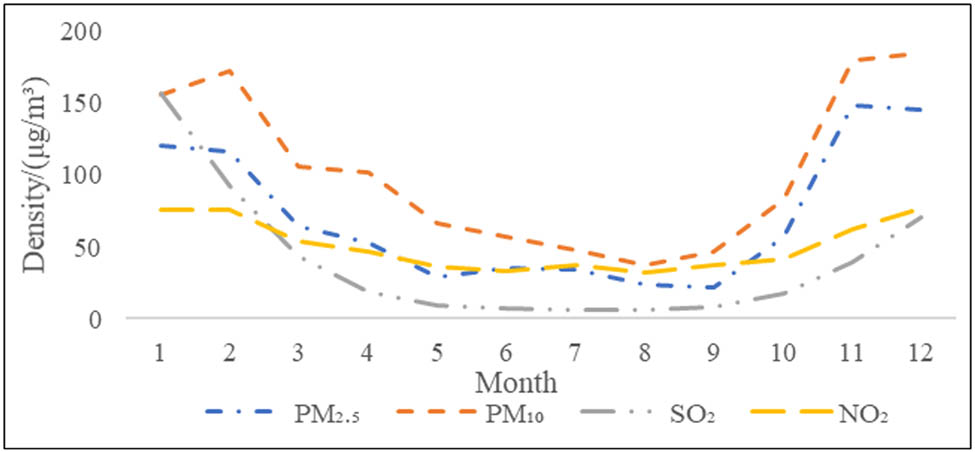
The distribution per month of major air pollutant concentrations in Harbin in 2015.
The average monthly PM2.5 concentration ranged between 22 and 149 µg/m3, with an average monthly concentration of 70.75 µg/m3.
The average monthly PM10 concentration ranged between 37 and 145 µg/m3, with an average monthly concentration of 103.42 µg/m3.
The average monthly SO2 concentration ranged between 6 and 157 µg/m3, with an average monthly concentration of 39.67 µg/m3.
The average monthly NO2 concentration ranged between 32 and 77 µg/m3, with an average monthly concentration of 50.75 µg/m3.
Figure 2 shows the statistics of air quality during haze in Harbin in 2015. During November, heavy pollution and above pollution occurred continuously in Harbin, mainly concentrated in early November; the number of days for air quality compliance was only 8 days, mainly in the middle of November. In December, there was a serious decline in air quality, with severe pollution and above days reaching 13 days, concentrated in the middle and end of the month stages. The number of days to reach the standard was less than in November, at only 6 days. During January 2016, there was a phenomenon of “returning to temperature” in the air quality, no severe pollution occurred, the number of days of heavy pollution decreased, and the number of days of compliance increased significantly.

Calendar distribution of 2015 winter air quality.
4.3 Analysis of air quality in winter 2016
In 2016, there were 358 days of effective air quality monitoring in Harbin, and the ratio of air quality to standard days was 77.7%. The proportion of days with excellent air quality was 28.8%, the proportion of days with good air quality was 48.9%, the proportion of days with light pollution was 15.6%, the proportion of moderate pollution days was 4.2%, and the proportion of severe pollution days was 2.2%.
The average concentration of air pollutants in each month in 2016 are finished and mapped as shown in Figure 3. In January, all pollutants were in the peak period, and the PM2.5 increased sharply, while the PM10 monthly average concentration surpassed 100. SO2 increased rapidly during the winter and peaked in January, followed by a rapid decline; over time there were small ups and downs, but the overall trend is declining. In June, July, and August, the concentration of all pollutants was at the lowest stage of the year. Since September, the concentrations of various pollutants showed an upward trend, and in November, PM2.5 increased sharply. The average concentration of PM10 exceeded 100, SO2 and NO2 also increased, and NO2 fluctuated little year-round. The details are as follows:
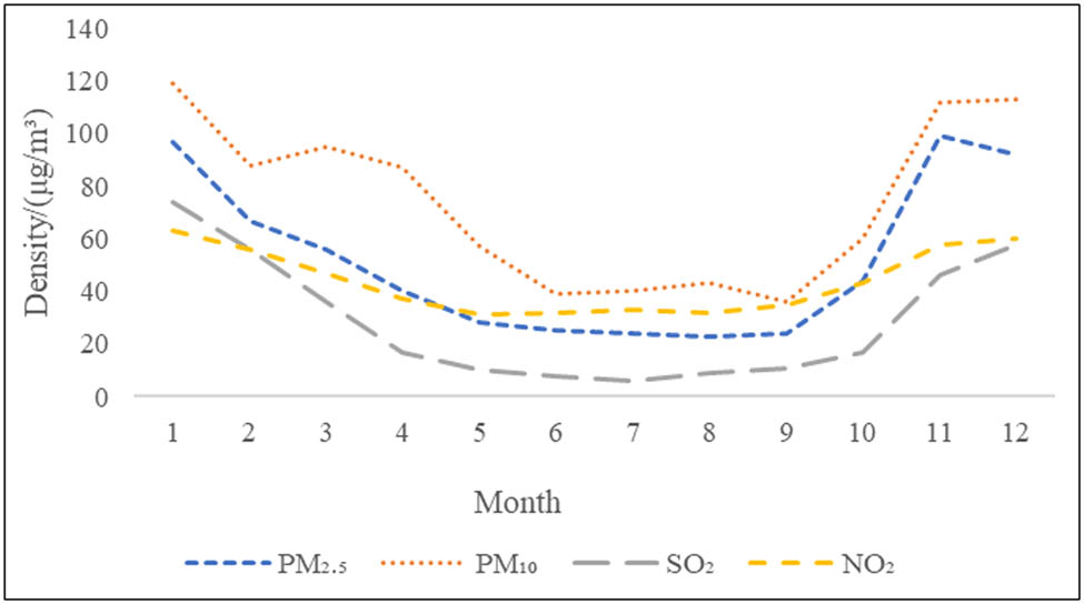
The distribution per month of major air pollutant concentrations in Harbin in 2016.
The average monthly PM2.5 concentration ranged between 23 and 99 µg/m3, with an average monthly concentration of 51.58 µg/m3.
The average monthly PM10 concentration ranged between 36 and 119 µg/m3, with an average monthly concentration of 74.10 µg/m3.
The average monthly SO2 concentration ranged between 6 and 74 µg/m3, with an average monthly concentration of 29 µg/m3.
The average monthly NO2 concentration ranged between 31 and 63 µg/m3, with an average monthly concentration of 43.92 µg/m3.
The air quality statistics during the winter of 2016 are shown in Figure 4. It can be seen that compared with the same period in winter 2015, Harbin’s days of heavy pollution decreased from 25 to 17 days, a decrease of 32%, and the number of days of compliance increased from 27 to 37 days, an increase of 27.1%, meaning that the air quality has greatly improved. In November and December, nearly half of the days met targets, but by January 2017, the days above severe pollution increased, and the concentration of all pollutants reached the maximum mainly in early January and late mid-January.

Calendar distribution of 2016 winter air quality.
4.4 Analysis of air quality in winter 2017
In 2017, Harbin city monitored 365 days of effective air quality, and the proportion of air quality standards reached 74%. The proportion of days with excellent air quality was 25.5%, the proportion of days with good air quality was 48.5%, the proportion of days with mild pollution was 13.4%, the proportion of moderate pollution days was 4.4%, and the proportion of severe pollution days was 5.8%.
The average concentration of air pollutants in each month in 2017 is finished and mapped as shown in Figure 5. In 2017, the concentration of air pollutants fluctuated greatly compared with the previous 2 years. In January, all pollutants were in the peak period, and the monthly average concentration of PM2.5 and PM10 exceeded 100, reaching the highest peak in January; then, there was a small decrease, which fell during the period. However, the concentration reached a small peak in April and then declined rapidly. In June, July, and August, the concentration of all pollutants was at the lowest peak of the year; since September, the concentrations of various pollutants increased rapidly. In October, the concentrations of PM2.5 and PM10 increased rapidly and reached the next highest peak, followed by a downward trend. SO2 and NO2 increased during the winter period, and the fluctuations were small.
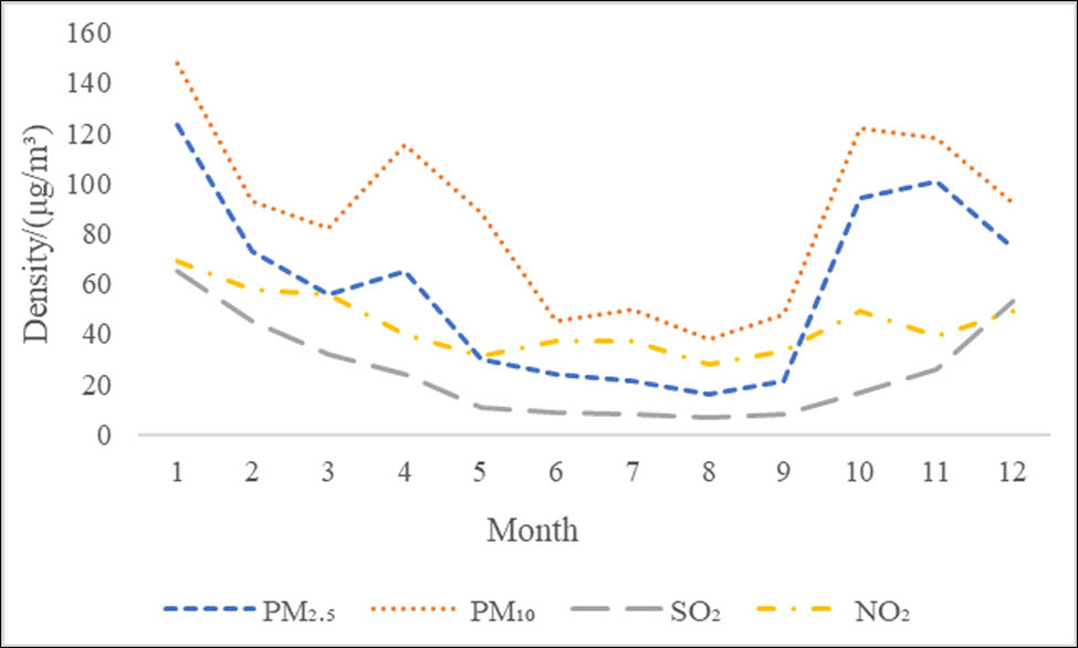
The distribution per month of major air pollutant concentrations in Harbin in 2017.
The average monthly PM2.5 concentration ranged between 16 and 123 µg/m3, with an average monthly concentration of 58.2 µg/m3.
The average monthly PM10 concentration ranged between 38 and 148 µg/m3, with an average monthly concentration of 86.58 µg/m3.
The average monthly SO2 concentration ranged between 7 and 65 µg/m3, with an average monthly concentration of 25.42 µg/m3.
The average monthly NO2 concentration ranged between 28 and 69 µg/m3, with an average monthly concentration of 43.83 µg/m3.
To sort out the air quality during the winter of 2017, as shown in Figure 6, compared with the same period in the winter of 2015, Harbin’s severe pollution and above days decreased from 25 to 9 days, a decrease of 64%, and the number of days of compliance increased from 27 to 56 days, an increase of 51.8%. Compared with the same period in winter 2016, severe pollution and above days decreased from 17 to 9 days, a decrease of 47.1%, and the number of days of compliance increased from 37 to 56 days, an increase of 34%, meaning that the air quality has obviously improved. In the winter of 2017, the most serious pollution of air quality was concentrated in the beginning of November. The air quality in the week was more than severe pollution.

Calendar distribution of 2017 winter air quality.
Combined with the above chart, from the winter of 2015 to the winter of 2017, the overall air quality situation in Harbin has improved, and the number of severe pollution days has decreased year by year. The main air pollutants in winter are PM10 and PM2.5. In October and November, the pollution concentration peaked, and after December, it showed a downward trend until the spring reached the valley in the following spring.
5 Discussion
5.1 Analysis of the back trajectory of air masses
In this article, the HYSPLIT-4 model uses the GDAS meteorological data and UTC time to target the Harbin urban area (45.64°N–45.86°N, 126.47°E–126.81°E). The analysis of air quality in the past 3 years lasted for three consecutive years with severe conditions. The trajectories starting from 8 November 2015, 8 January 2017, and 7 November 2017 were selected as the starting point of the trajectory, and the 3 day (72 h) backward transportation trajectory was calculated by the model. The specific air mass trajectory is shown in Figure 7. The height of the air mass trajectory is selected from three different height levels. The red trajectory represents the altitude of 100 m, the blue trajectory represents the height of 1,000 m, and the green trajectory represents the air mass transport trajectory at a height of 1,500 m.
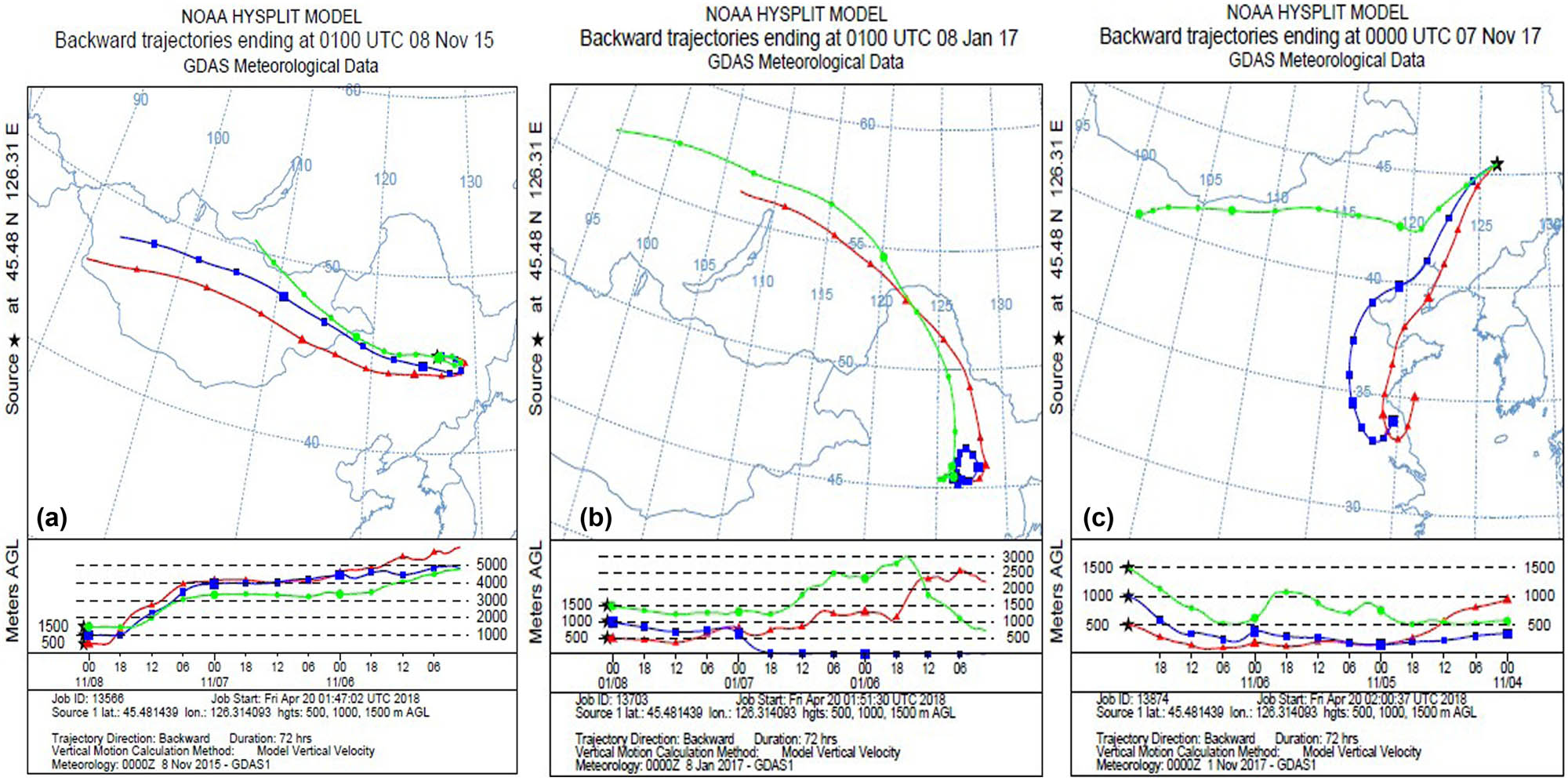
72 h trail of Harbin city: (a) 2015.11.08 UTC 01:00, (b) 2017.01.08 UTC 01:00, and (c) 2017.11.07 UTC 00:00.
Figure 7a is an analysis of the backward trajectory at 09:00 AM on 8 November 2015 (UTC time is 01:00 on 8 November). It can be seen that the three air masses are affected by the northwest monsoon, starting from the high altitudes of Mongolia and entering China’s Inner Mongolia at about 6:00 on 6 November; the air flow is relatively stable. Before 7 November, the air flow moved above 3,000 m altitude. Since 06:00 on 7 November, the air flow began to fluctuate. At the same time, air masses at different heights decreased. At 18:00, they stabilized, and the three air masses returned to their corresponding heights. At this time, the air masses moved to Mudanjiang city and were affected by surface air flow. The air masses entered the city of Harbin from east to west.
Figure 7b is an analysis of the backward trajectory at 09:00 AM on 8 January 2017 (UTC time 1 January, 01:00), as the picture shows; The air masses at 500 and 1,500 m heights moved from northwest to southeast, and the 1,500 m high air flow activity is active, starting from a 600 m altitude in Russia to move southeast; at about 18:00 on 5 January, it quickly rose to an altitude of 3,000 m, and then gradually decreased again. At 18:00 on 6 January, the air mass stabilized at an altitude of 1,500 m and arrived at the northern side of Harbin in the early morning of 7 January. During the daytime on 7 January, the air mass moved to the west side of Harbin, and then returned to Harbin. The 500 m air mass began to move from a height of 2,000 m, the airflow was weakening, and the height of the air mass continued to decrease. On 6 January, the air mass dropped to 1,500 m. At this time, the air mass entered the Greater Khingan Range and then moved from the northern side of Heilongjiang Province to the southeast. On the morning of 7 January, the air mass returned to the 500 m altitude and reached the east side of Harbin and entered Harbin from east to west. The air mass at a height of 1,000 m moved around Harbin from 6 to 8 January. During the period from 5 to 6 January, the air masses moved around the surface. On the morning of 7 January, the air mass began to rise and gradually returned to the altitude of 1,000 m.
Figure 7c shows an analysis of the backward trajectory at 08:00 on 7 November 2017 (UTC time is 00:00 on 7 November). As can be seen from the figure, this time, the air mass trajectory starts from the southwest of Harbin and moves from southwest to northeast. The air mass at the altitude of 1,500 m began to move from Inner Mongolia to Liaoning Province and Jilin Province, and finally entered Harbin City from the southwest side. The air masses had been moving at a high altitude near 500 m before 5 November, and they had risen to 1,000 m at 18:00 on the 5 November and then dropped to 500 m. At 12:00 on the 6 November, the air mass began to rise and gradually returned to 1,500 m. The air mass trajectories at the altitudes of 500 and 1,000 m were basically the same. On the morning of 4 to 12 November, the air mass moved southward from northern Jiangsu and then entered Harbin through Anhui, Shandong, Henan, Hebei, Shenyang, Jilin, and other provinces. The air mass at the height of 1,000 m began to move at a height of 500 m, during which the air flow was relatively stable. From 12:00 on 6 November, the air mass rose and gradually returned to 1,000 m. The air masses at a height of 500 m began to move from an altitude of 1,000 m, then fell to surface movement, and the air flow was always stable.
5.2 Analysis of straw incineration around Heilongjiang Province
In the northern provinces of China, there are many straw-burning phenomena in autumn, which combine with the climate characteristics and farming system of Heilongjiang Province, as well as the hysteresis of the pollution effect caused by straw burning. An analysis of straw burning in October and November in the past 2 years (due to the missing 2015 straw-burning data, this year is not analyzed) is shown in Figure 8.
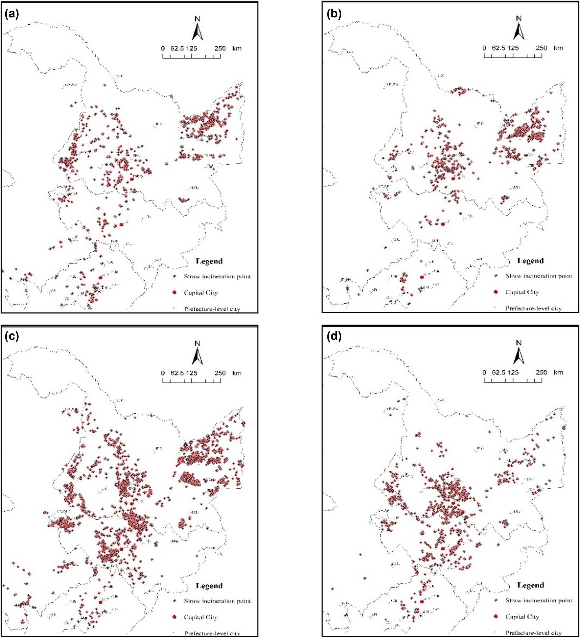
Distribution of straw-incineration points: (a) 2016.10, (b) 2016.11, (c) 2017.10, and (d) 2017.11.
Figure 8a shows the situation of straw burning around Heilongjiang Province in October 2016. It can be seen that the straw burning in October is mostly distributed in the northeastern region and North China and is more serious the northeastern region. Among them, Heilongjiang Province has the most concentrated burning, and the central and western regions are mostly concentrated in Harbin, Daqing, Suihua, and Qiqihar. Burning in the east is mostly concentrated in Jiamusi city and Shuangyashan city. The burning points in Jilin Province are concentrated in the surrounding areas of Baicheng and Changchun, and the burning points in Liaoning Province are concentrated around Panjin and Liaoyang. Figure 8b shows the situation of straw incineration around Heilongjiang Province in November 2016. It can be seen from the figure that the situation of straw burning in the northeast region has improved compared with that in October, Jilin Province and Liaoning Province have significantly decreased, and Heilongjiang Province has decreased. However, the approximate distribution is basically similar to that in October. Figure 8c shows the situation of straw burning around Heilongjiang Province in October 2017. Compared with October 2016, the straw burning in the northeast region has intensified, and straw burning has occurred in nearly half of Heilongjiang Province and Jilin Province. The straw burning in Heilongjiang Province is divided into two major regions, and the central and western regions are mostly distributed in Harbin, Suihua, Daqing, and Qiqihar. In the eastern region, there are different degrees of straw burning, among which Jiamusi city and Hegang city are the most serious. Figure 8d shows the situation of straw burning around Heilongjiang Province in November 2017. Compared with October 2017, it can be clearly seen that the number of straw-burning points in Northeast China has decreased.
By analyzing the distribution of straw incineration points, it can be found that the backward trajectory path partially overlaps with the distribution range of straw incineration sites in the surrounding areas of Heilongjiang Province. The air mass movement transported pollutants from straw incineration to Harbin, and because Harbin was located in the Mongolian high-pressure zone in winter, the air mass affected by surface and weather was likely to gather in the sky, causing the easy formation of smog.
6 Conclusion
In recent years, the smog phenomenon in Harbin has occurred frequently in winter, which has caused great problems for the living environment of local residents. To trace the causes of smog, the Ministry of Ecology and Environment of the People’s Republic of China and the Environmental Protection Department of Heilongjiang Province have used air quality data and straw-burning data based on the latest environmental quality standard (GB3095-2012) promulgated by the Ministry of Environmental Protection and Environmental Protection in 2012; the formula calculates the monthly major pollutants according to the 74 city air quality status reports issued by the Ministry of Ecology and Environment of the People’s Republic of China. Finally, the concentration changes of four pollutants of PM2.5, PM10, SO2, and NO2 in the past 3 years were analyzed. It was found that the concentration of each pollutant increased sharply from November and began to decline in March of the following year. It is found that air pollution is the most serious in November every year and is most prone to continuous pollution at the beginning of the month.
The HYSPLIT-4 model was used to analyze the cause of the sharp increase in pollutant concentration. The atmospheric movement of the most severe period of pollution in Harbin was selected. It was found that the trajectory of the air mass was affected by the northwest monsoon. The air mass mainly entered from the west side of Harbin. Taking into account the current situation of agricultural activities in the northeast region, the corn stalk-burning period occurs at that time, and the national straw-burning point is transferred through the Ministry of Ecology and Environment of the People’s Republic of China, focusing on the distribution of straw-burning points in the northeast region, and it is found that the burning of straw in Heilongjiang Province is serious. The time period is concentrated in October and November, and the distribution of straw-burning points on the west side of Harbin is relatively concentrated, which coincides with the air tracking.
Using the air quality index, straw-burning point, and HYSPLIT-4 model to analyze the air pollution causes of Harbin in the past 3 years, it is found that the main pollutant in winter is PM2.5. One of the causes of smog is straw burning in October and November each year. In addition, the winter in Harbin is affected by the northwest monsoon in winter. It is located on the edge of the high-pressure area of the mainland, and the air movement of pollution and the transportation of goods to low altitudes has aggravated the haze phenomenon in Harbin. Therefore, one of the causes of the serious haze in winter in Harbin in recent years is the transport of fine particles produced by the burning of surrounding straw.
In the next research process, the effects of hot spot distribution will be analyzed and an exhaust gas emissions analysis of haze will be conducted in Harbin.
Acknowledgements
The authors would like to express gratitude to the research grant support kindly provided by the National Natural Science Foundation of China (Grant No. 42171246, 41101177), China Postdoctoral Science Foundation (Grant No. 2017M621229), Postdoctoral Science Foundation of Heilongjiang Province (Grant No. LBH-Z17001), Philosophy and social science program in Heilongjiang Province (Grant No. 21GLB061), Heilongjiang Research Fund for Returned Overseas Students, Key Research and Development Program of Heilongjiang Province (Grant No. GZ20210193), and 2021 Science and Technology Innovation Think Tank Research Project of Heilongjiang Association for Science and Technology.
-
Funding information: This research was funded by the National Natural Science Foundation of China (Grant No. 42171246, 41101177), China Postdoctoral Science Foundation (Grant No. 2017M621229), Postdoctoral Science Foundation of Heilongjiang Province (Grant No. LBH-Z17001), Philosophy and social science program in Heilongjiang Province (Grant No. 21GLB061), Key Research and Development Program of Heilongjiang Province (Grant No. GZ20210193), and 2021 Science and Technology Innovation Think Tank Research Project of Heilongjiang Association for Science and Technology.
-
Author contributions: LW was responsible for the research design and guiding the writing and publication of the article; JRD wrote the first draft of the article; LJY modified the text and format of the article; and YLY and DWX reviewed the article and provided feedback.
-
Conflict of interest: The authors declare no conflict of interest.
References
[1] Lukić T, Gavrilov MB, Marković SB, Zorn M, Komac B, Mladjan D, et al. Classification of the natural disasters between the legislation and application: experience of the Republic of Serbia. Acta Geographica Slovenica. 2013;53-1:149–64. 10.3986/AGS53301.Suche in Google Scholar
[2] Filonchyk M, Peterson M. Air quality changes in Shanghai, China, and the surrounding urban agglomeration during the COVID-19 lockdown. J Geovisualization Spat Anal. 2020;4(22):22. 10.1007/s41651-020-00064-5.Suche in Google Scholar
[3] Huang Y, Yan Q, Zhang C. Spatial–temporal distribution characteristics of PM2.5 in China in 2016. J Geovis Spat Anal. 2018;2(2):1–8. 10.1007/s41651-018-0019-5.Suche in Google Scholar
[4] Liang Z, Zhou C, Fan Y, Lei C, Sun D. Spatio-temporal evolution and the influencing factors of PM2.5 in China between 2000 and 2015. J Geograph Sci. 2019;29(2):253–70. 10.1007/s11442-019-1595-0.Suche in Google Scholar
[5] Lelieveld J, Evans JS, Fnais M, Giannadaki D, Pozzer A. The contribution of outdoor air pollution sources to premature mortality on a global scale. Nature. 2015;525(7569):367–71. 10.1038/NATURE15371.Suche in Google Scholar
[6] Brock WA, Taylor MS. Chapter 28 – economic growth and the environment: a review of theory and empirics. In: Aghion P, Durlauf SN, editors. Handbook of economic growth. 1. Elsevier; 2005. p. 1749–821. 10.1016/S1574-0684(05)01028-2.Suche in Google Scholar
[7] Al-Mulali U, Ozturk I. The investigation of environmental Kuznets curve hypothesis in the advanced economies: the role of energy prices. Renew Sust Energ Rev. 2016;54:1622–31. 10.1016/j.rser.2015.10.131.Suche in Google Scholar
[8] Damette O, Delacote P, Lo GD. Households energy consumption and transition toward cleaner energy sources. Energy Policy. 2018;113:751–64. 10.1016/j.empol.2017.10.060.Suche in Google Scholar
[9] Vassanadumrongdee S, Matsuoka S, Shirakawa H. Meta-analysis of contingent valuation studies on air pollution-related morbidity risks. Environ Econ and Policy Studies. 2004;6(1):11–47. 10.1007/BF03353929.Suche in Google Scholar
[10] Kampa M, Castanas E. Human health effects of air pollution. Environ Pollut. 2008;151(2):362–7. 10.1016/j.envpol.2007.06.012.Suche in Google Scholar PubMed
[11] Saez M, Lopez-Casasnovas G. Assessing the effects on health inequalities of differential exposure and differential susceptibility of air pollution and environmental noise in Barcelona, 2007–2014. Inter J Env Res Pub Hea. 2019;16(18):3470–93. 10.3390/ijerph16183470.Suche in Google Scholar
[12] Soleimani Z, Darvishi Boloorani A, Khalifeh R, Griffin DW, Mesdaghinia A. Short-term effects of ambient air pollution and cardiovascular events in Shiraz, Iran, 2009 to 2015. Environ SCI Pollut R. 2019;26(7):6359–67. 10.1007/S11356-018-3952-4.Suche in Google Scholar
[13] Hu J, Ying Q, Wang Y, Zhang H. Characterizing multi-pollutant air pollution in China: Comparison of three air quality indices. Environ Int. 2015;84:17–25. 10.1016/j.envint.2015.06.014.Suche in Google Scholar
[14] MEP. “Ambient Air Quality Standards GB3095-2012”, Beijing, China (In Chinese); 2012.Suche in Google Scholar
[15] Appel BR, Tokiwa Y, Hsu J, Kothny EL, Hahn E. Visibility as related to atmospheric aerosol constituents. Atmos Environ (1967). 1985;19(9):1525–34. 10.1016/0004-6981(85)90290-2.Suche in Google Scholar
[16] Marcazzan GM, Vaccaro S, Valli G, Vecchi R. Characterisation of PM10 and PM2.5 particulate matter in the ambient air of Milan (Italy). Atmos Environ. 2001;35(27):4639–50. 10.1016/S1352-2310(01)00124-8.Suche in Google Scholar
[17] Kulshrestha A, Satsangi PG, Masih J, Taneja A. Metal concentration of PM2.5 and PM10 particles and seasonal variations in urban and rural environment of Agra, India. Sci Total Environ. 2009;407(24):6196–204. 10.1016/j.scitotenv.2009.08.050.Suche in Google Scholar PubMed
[18] Seinfeld JH, Pandis SN. Atmospheric chemistry and physics: from air pollution to climate change. New York: John Wiley & Sons; 2016.Suche in Google Scholar
[19] Gautam R. Challenges in early warning of the persistent and widespread winter fog over the Indo-Gangetic plains: a satellite perspective. Dordrecht: Springer; 2014. p. 51–61. 10.1007/978-94-017-8598-3_3.Suche in Google Scholar
[20] Sánchez de la Campa AM, Sánchez-Rodas D, Alsioufi L, Alastuey A, Querol X, De la Rosa JD. Air quality trends in an industrialised area of SW Spain. J Clean Prod. 2018;186:465–74. 10.1016/j.jclepro.2018.03.122.Suche in Google Scholar
[21] Viana M, Hammingh P, Colette A, Querol X, Degraeuwe B, Vlieger I, et al. Impact of maritime transport emissions on coastal air quality in Europe. Atmos Environ. 2014;90:96–105. 10.1016/j.atmosenv.2014.03.046.Suche in Google Scholar
[22] Lin XQ, Wang D. Spatiotemporal evolution of urban air quality and socioeconomic driving forces in China. J Geogr Sci. 2016;26(11):1533–49. 10.1007/S11442-016-1342-8.Suche in Google Scholar
[23] Wang J-F, Zhang T-L, Fu B-J. A measure of spatial stratified heterogeneity. Ecol Indic. 2016;67:250–6. 10.1016/j.ecolind.2016.02.052.Suche in Google Scholar
[24] Fang CL, Wang ZB, Xu G. Spatial-temporal characteristics of PM2.5 in China: a city-level perspective analysis. J Geogr Sci. 2016;26(11):1519–32. 10.1007/S11442-016-1341-9.Suche in Google Scholar
[25] Gong ZZ, Zhang XP. Assessment of Urban Air Pollution and Spatial Spillover Effects in China: Cases of 113 Key Environmental Protection Cities. JRE. 2017;8(6):584–94. 10.5814/j.issn.1674-764x.2017.06.004.Suche in Google Scholar
[26] Cavalcante RM, Rocha CA, De Santiago ÍS, Da Silva TFA, Cattony CM, Silva MVC, et al. Influence of urbanization on air quality based on the occurrence of particle-associated polycyclic aromatic hydrocarbons in a tropical semiarid area (Fortaleza-CE, Brazil). Air Qual, Atmos Hlth. 2017;10(4):437–45. 10.1007/S11869-016-0434-Z.Suche in Google Scholar
[27] Tai APK, Mickley LJ, Jacob DJ. Correlations between fine particulate matter (PM2.5) and meteorological variables in the United States: implications for the sensitivity of PM2.5 to climate change. Atmos Environ. 2010;44(32):3976–84. 10.1016/j.atmosenv.2010.06.060.Suche in Google Scholar
[28] Sun L, Wei J, Duan DH, Guo YM, Yang DX, Jia C, et al. Impact of land-use and land-cover change on urban air quality in representative cities of China. J Atmos Sol-Terr Phy. 2016;142:43–54. 10.1016/j.jastp.2016.02.022.Suche in Google Scholar
[29] Zou B, Xu S, Sternberg T, Fang X. Effect of land use and cover change on air quality in urban sprawl. Sustainability. 2016;8(7):677–90. 10.3390/SU8070677.Suche in Google Scholar
[30] Dinda S, Coondoo D, Pal M. Air quality and economic growth: an empirical study. Ecol Econ. 2000;34(3):409–23. 10.1016/S0921-8009(00)00179-8.Suche in Google Scholar
[31] Shaw D, Pang A, Lin C-C, Hung M-F. Economic growth and air quality in China. Environ Econ Policy Studies. 2010;12(3):79–96. 10.1007/S10018-010-0166-5.Suche in Google Scholar
[32] Orubu CO, Omotor DG. Environmental quality and economic growth: Searching for environmental Kuznets curves for air and water pollutants in Africa. Energy Policy. 2011;39(7):4178–88. 10.1016/j.enpol.2011.04.025.Suche in Google Scholar
[33] Patton AP, Perkins J, Zamore W, Levy JI, Brugge D, Durant JL. Spatial and temporal differences in traffic-related air pollution in three urban neighborhoods near an interstate highway. Atmos Environ. 2014;99:309–21. 10.1016/j.atmosenv.2014.09.072.Suche in Google Scholar PubMed PubMed Central
[34] Friedman MS, Powell KE, Hutwagner L, Graham LM, Teague WG. Impact of changes in transportation and commuting behaviors during the 1996 summer Olympic games in Atlanta on air quality and childhood asthma. JAMA. 2001;285(7):897–905. 10.1001/jama.285.7.897.Suche in Google Scholar PubMed
[35] Kinnon MM, Zhu S, Carreras-Sospedra M, Soukup JV, Dabdub D, Samuelsen GS, et al. Considering future regional air quality impacts of the transportation sector. Energy Policy. 2019;124:63–80. 10.1016/j.enpol.2018.09.011.Suche in Google Scholar
[36] Zhang H, Wang S, Hao J, Wang X, Wang S, Chai F, et al. Air pollution and control action in Beijing. J Clean Prod. 2016;112:1519–27. 10.1016/j.jclepro.2015.04.092.Suche in Google Scholar
[37] Xie XY, Tou XD, Zhang L. Effect analysis of air pollution control in Beijing based on an odd-and-even license plate model. J Clean Production. 2017;142:936–45. 10.1016/j.jclepro.2016.09.117.Suche in Google Scholar
[38] Hu JL, Wang YG, Ying Q, Zhang HL. Spatial and temporal variability of PM2.5 and PM10 over the North China Plain and the Yangtze River Delta, China. Atmos Environ. 2014;95:598–609. 10.1016/j.atmosenv.2014.07.019.Suche in Google Scholar
[39] Gavrilov MB. Integration of the shallow water equations in a plane geometry using semi-Lagrangian and Eulerian schemes. Meteorol Atmos Phys. 1997;62:141–60. 10.1007/BF01029699.Suche in Google Scholar
[40] Draxler RR. HYSPLIT (HYbrid Single-Particle Lagrangian Integrated Trajectory) Model access via NOAAARL READY Website; 2003.Suche in Google Scholar
[41] Zhang JY, Song SH, Wen JH, Wen JH. Source of airborne particulate matter in guilin based on backward trajectory model. Environ Monit China. 2017;33(2):42–6. 10.19316/j.issn.1002-6002.2017.02.07.Suche in Google Scholar
© 2021 Lei Wang et al., published by De Gruyter
This work is licensed under the Creative Commons Attribution 4.0 International License.
Artikel in diesem Heft
- Regular Articles
- Lithopetrographic and geochemical features of the Saalian tills in the Szczerców outcrop (Poland) in various deformation settings
- Spatiotemporal change of land use for deceased in Beijing since the mid-twentieth century
- Geomorphological immaturity as a factor conditioning the dynamics of channel processes in Rządza River
- Modeling of dense well block point bar architecture based on geological vector information: A case study of the third member of Quantou Formation in Songliao Basin
- Predicting the gas resource potential in reservoir C-sand interval of Lower Goru Formation, Middle Indus Basin, Pakistan
- Study on the viscoelastic–viscoplastic model of layered siltstone using creep test and RBF neural network
- Assessment of Chlorophyll-a concentration from Sentinel-3 satellite images at the Mediterranean Sea using CMEMS open source in situ data
- Spatiotemporal evolution of single sandbodies controlled by allocyclicity and autocyclicity in the shallow-water braided river delta front of an open lacustrine basin
- Research and application of seismic porosity inversion method for carbonate reservoir based on Gassmann’s equation
- Impulse noise treatment in magnetotelluric inversion
- Application of multivariate regression on magnetic data to determine further drilling site for iron exploration
- Comparative application of photogrammetry, handmapping and android smartphone for geotechnical mapping and slope stability analysis
- Geochemistry of the black rock series of lower Cambrian Qiongzhusi Formation, SW Yangtze Block, China: Reconstruction of sedimentary and tectonic environments
- The timing of Barleik Formation and its implication for the Devonian tectonic evolution of Western Junggar, NW China
- Risk assessment of geological disasters in Nyingchi, Tibet
- Effect of microbial combination with organic fertilizer on Elymus dahuricus
- An OGC web service geospatial data semantic similarity model for improving geospatial service discovery
- Subsurface structure investigation of the United Arab Emirates using gravity data
- Shallow geophysical and hydrological investigations to identify groundwater contamination in Wadi Bani Malik dam area Jeddah, Saudi Arabia
- Consideration of hyperspectral data in intraspecific variation (spectrotaxonomy) in Prosopis juliflora (Sw.) DC, Saudi Arabia
- Characteristics and evaluation of the Upper Paleozoic source rocks in the Southern North China Basin
- Geospatial assessment of wetland soils for rice production in Ajibode using geospatial techniques
- Input/output inconsistencies of daily evapotranspiration conducted empirically using remote sensing data in arid environments
- Geotechnical profiling of a surface mine waste dump using 2D Wenner–Schlumberger configuration
- Forest cover assessment using remote-sensing techniques in Crete Island, Greece
- Stability of an abandoned siderite mine: A case study in northern Spain
- Assessment of the SWAT model in simulating watersheds in arid regions: Case study of the Yarmouk River Basin (Jordan)
- The spatial distribution characteristics of Nb–Ta of mafic rocks in subduction zones
- Comparison of hydrological model ensemble forecasting based on multiple members and ensemble methods
- Extraction of fractional vegetation cover in arid desert area based on Chinese GF-6 satellite
- Detection and modeling of soil salinity variations in arid lands using remote sensing data
- Monitoring and simulating the distribution of phytoplankton in constructed wetlands based on SPOT 6 images
- Is there an equality in the spatial distribution of urban vitality: A case study of Wuhan in China
- Considering the geological significance in data preprocessing and improving the prediction accuracy of hot springs by deep learning
- Comparing LiDAR and SfM digital surface models for three land cover types
- East Asian monsoon during the past 10,000 years recorded by grain size of Yangtze River delta
- Influence of diagenetic features on petrophysical properties of fine-grained rocks of Oligocene strata in the Lower Indus Basin, Pakistan
- Impact of wall movements on the location of passive Earth thrust
- Ecological risk assessment of toxic metal pollution in the industrial zone on the northern slope of the East Tianshan Mountains in Xinjiang, NW China
- Seasonal color matching method of ornamental plants in urban landscape construction
- Influence of interbedded rock association and fracture characteristics on gas accumulation in the lower Silurian Shiniulan formation, Northern Guizhou Province
- Spatiotemporal variation in groundwater level within the Manas River Basin, Northwest China: Relative impacts of natural and human factors
- GIS and geographical analysis of the main harbors in the world
- Laboratory test and numerical simulation of composite geomembrane leakage in plain reservoir
- Structural deformation characteristics of the Lower Yangtze area in South China and its structural physical simulation experiments
- Analysis on vegetation cover changes and the driving factors in the mid-lower reaches of Hanjiang River Basin between 2001 and 2015
- Extraction of road boundary from MLS data using laser scanner ground trajectory
- Research on the improvement of single tree segmentation algorithm based on airborne LiDAR point cloud
- Research on the conservation and sustainable development strategies of modern historical heritage in the Dabie Mountains based on GIS
- Cenozoic paleostress field of tectonic evolution in Qaidam Basin, northern Tibet
- Sedimentary facies, stratigraphy, and depositional environments of the Ecca Group, Karoo Supergroup in the Eastern Cape Province of South Africa
- Water deep mapping from HJ-1B satellite data by a deep network model in the sea area of Pearl River Estuary, China
- Identifying the density of grassland fire points with kernel density estimation based on spatial distribution characteristics
- A machine learning-driven stochastic simulation of underground sulfide distribution with multiple constraints
- Origin of the low-medium temperature hot springs around Nanjing, China
- LCBRG: A lane-level road cluster mining algorithm with bidirectional region growing
- Constructing 3D geological models based on large-scale geological maps
- Crops planting structure and karst rocky desertification analysis by Sentinel-1 data
- Physical, geochemical, and clay mineralogical properties of unstable soil slopes in the Cameron Highlands
- Estimation of total groundwater reserves and delineation of weathered/fault zones for aquifer potential: A case study from the Federal District of Brazil
- Characteristic and paleoenvironment significance of microbially induced sedimentary structures (MISS) in terrestrial facies across P-T boundary in Western Henan Province, North China
- Experimental study on the behavior of MSE wall having full-height rigid facing and segmental panel-type wall facing
- Prediction of total landslide volume in watershed scale under rainfall events using a probability model
- Toward rainfall prediction by machine learning in Perfume River Basin, Thua Thien Hue Province, Vietnam
- A PLSR model to predict soil salinity using Sentinel-2 MSI data
- Compressive strength and thermal properties of sand–bentonite mixture
- Age of the lower Cambrian Vanadium deposit, East Guizhou, South China: Evidences from age of tuff and carbon isotope analysis along the Bagong section
- Identification and logging evaluation of poor reservoirs in X Oilfield
- Geothermal resource potential assessment of Erdaobaihe, Changbaishan volcanic field: Constraints from geophysics
- Geochemical and petrographic characteristics of sediments along the transboundary (Kenya–Tanzania) Umba River as indicators of provenance and weathering
- Production of a homogeneous seismic catalog based on machine learning for northeast Egypt
- Analysis of transport path and source distribution of winter air pollution in Shenyang
- Triaxial creep tests of glacitectonically disturbed stiff clay – structural, strength, and slope stability aspects
- Effect of groundwater fluctuation, construction, and retaining system on slope stability of Avas Hill in Hungary
- Spatial modeling of ground subsidence susceptibility along Al-Shamal train pathway in Saudi Arabia
- Pore throat characteristics of tight reservoirs by a combined mercury method: A case study of the member 2 of Xujiahe Formation in Yingshan gasfield, North Sichuan Basin
- Geochemistry of the mudrocks and sandstones from the Bredasdorp Basin, offshore South Africa: Implications for tectonic provenance and paleoweathering
- Apriori association rule and K-means clustering algorithms for interpretation of pre-event landslide areas and landslide inventory mapping
- Lithology classification of volcanic rocks based on conventional logging data of machine learning: A case study of the eastern depression of Liaohe oil field
- Sequence stratigraphy and coal accumulation model of the Taiyuan Formation in the Tashan Mine, Datong Basin, China
- Influence of thick soft superficial layers of seabed on ground motion and its treatment suggestions for site response analysis
- Monitoring the spatiotemporal dynamics of surface water body of the Xiaolangdi Reservoir using Landsat-5/7/8 imagery and Google Earth Engine
- Research on the traditional zoning, evolution, and integrated conservation of village cultural landscapes based on “production-living-ecology spaces” – A case study of villages in Meicheng, Guangdong, China
- A prediction method for water enrichment in aquifer based on GIS and coupled AHP–entropy model
- Earthflow reactivation assessment by multichannel analysis of surface waves and electrical resistivity tomography: A case study
- Geologic structures associated with gold mineralization in the Kirk Range area in Southern Malawi
- Research on the impact of expressway on its peripheral land use in Hunan Province, China
- Concentrations of heavy metals in PM2.5 and health risk assessment around Chinese New Year in Dalian, China
- Origin of carbonate cements in deep sandstone reservoirs and its significance for hydrocarbon indication: A case of Shahejie Formation in Dongying Sag
- Coupling the K-nearest neighbors and locally weighted linear regression with ensemble Kalman filter for data-driven data assimilation
- Multihazard susceptibility assessment: A case study – Municipality of Štrpce (Southern Serbia)
- A full-view scenario model for urban waterlogging response in a big data environment
- Elemental geochemistry of the Middle Jurassic shales in the northern Qaidam Basin, northwestern China: Constraints for tectonics and paleoclimate
- Geometric similarity of the twin collapsed glaciers in the west Tibet
- Improved gas sand facies classification and enhanced reservoir description based on calibrated rock physics modelling: A case study
- Utilization of dolerite waste powder for improving geotechnical parameters of compacted clay soil
- Geochemical characterization of the source rock intervals, Beni-Suef Basin, West Nile Valley, Egypt
- Satellite-based evaluation of temporal change in cultivated land in Southern Punjab (Multan region) through dynamics of vegetation and land surface temperature
- Ground motion of the Ms7.0 Jiuzhaigou earthquake
- Shale types and sedimentary environments of the Upper Ordovician Wufeng Formation-Member 1 of the Lower Silurian Longmaxi Formation in western Hubei Province, China
- An era of Sentinels in flood management: Potential of Sentinel-1, -2, and -3 satellites for effective flood management
- Water quality assessment and spatial–temporal variation analysis in Erhai lake, southwest China
- Dynamic analysis of particulate pollution in haze in Harbin city, Northeast China
- Comparison of statistical and analytical hierarchy process methods on flood susceptibility mapping: In a case study of the Lake Tana sub-basin in northwestern Ethiopia
- Performance comparison of the wavenumber and spatial domain techniques for mapping basement reliefs from gravity data
- Spatiotemporal evolution of ecological environment quality in arid areas based on the remote sensing ecological distance index: A case study of Yuyang district in Yulin city, China
- Petrogenesis and tectonic significance of the Mengjiaping beschtauite in the southern Taihang mountains
- Review Articles
- The significance of scanning electron microscopy (SEM) analysis on the microstructure of improved clay: An overview
- A review of some nonexplosive alternative methods to conventional rock blasting
- Retrieval of digital elevation models from Sentinel-1 radar data – open applications, techniques, and limitations
- A review of genetic classification and characteristics of soil cracks
- Potential CO2 forcing and Asian summer monsoon precipitation trends during the last 2,000 years
- Erratum
- Erratum to “Calibration of the depth invariant algorithm to monitor the tidal action of Rabigh City at the Red Sea Coast, Saudi Arabia”
- Rapid Communication
- Individual tree detection using UAV-lidar and UAV-SfM data: A tutorial for beginners
- Technical Note
- Construction and application of the 3D geo-hazard monitoring and early warning platform
- Enhancing the success of new dams implantation under semi-arid climate, based on a multicriteria analysis approach: Case of Marrakech region (Central Morocco)
- TRANSFORMATION OF TRADITIONAL CULTURAL LANDSCAPES - Koper 2019
- The “changing actor” and the transformation of landscapes