GIS and geographical analysis of the main harbors in the world
-
Aleksandar Valjarević
 ,
Dragan Radovanović
,
Dragan Radovanović

Abstract
This paper points out the possibilities of better exploitation of marine traffic as well as its connection with other kinds of traffic. Special attention is given to the analysis of 1,081 harbors about their availability during the year. The methods and algorithms used in GIS are buffers, cluster, method of interpolations, and network analysis. The methods used for the purpose of conducting numerical analyses are algorithms that served for the analysis of the network, its transport features, and the connectivity with harbors in terms of geospace. The main results found in this research showed that harbors have good connectivity in the first place with road traffic and after that with air and railroad traffic. According to data from 2019, all traffic lines cover 4.1 × 10¹⁵ km, and the road traffic has the most significant potential in connection with the harbors. The most connected harbors and airports are in the east coast of North America, west coast, north Europe, southern Europe, south-east Australia, a central part of Oceania, and south-east Africa. The results in the modified Likert scale between airports and harbors showed medium results. The densest road network is located in the eastern part of USA, western and central part of Europe, and east coast of China. The number of possible connected lines between main road nodes and harbors is 0.8 × 10⁹. This type of traffic showed excellent results and connection with harbors. The number of possible connected lines per month between railroads and harbors is 1.3 × 10³. This type of traffic showed low connectivity with the harbors. In the end comparison of harbors with air, road and railroad networks were established. The geographical position of harbors was analyzed, and better understanding was performed on a global scale.
1 Introduction
The position of the harbors, along with the influence of anthropogenic and natural factors, may be of great significance for the further development of marine traffic. The analysis of regions about cargo traffic sets a good example of how global marrine traffic should be treated [1]. The application of two algorithms such as Infomap and Walktrap could explain the interaction between the city harbors and the cities by means of road and railroad networks [2]. Geoinformatics and the application of GIS could be the new approach to study more efficient exploitation of harbors. India, which is becoming one of the leading world economies, will be strongly oriented to the exploitation of the sea harbors. This study has shown that by means of the analysis of the main export harbors as well as by the analysis of container export in the USA, it is possible to define the advantages and disadvantages of the harbors themselves [3].
In the last decades, the ports in the hugely populated areas have developed large cities. These cities are called hub cities because the development of ports affected the development of cities. Agglomerations and humankind itself move to shorelines of the world seas. At the same time, traffic was concentrated in these hub cities [4]. Port cities are some of the most economically strong and competitive cities in the world. However, a weakening of the ties between ports and cities has been identified over recent decades. This situation includes a very poor connection between ports and periphery regions close to ports. This region may be divided into three belts: first is the central area of port, second is the suburban part of the city, and third is the urban part of the city. Only ports (harbors) with good traffic and effective routes can be enough exploited [5]. A port-city system is a complex and integral system, and it can be simulated by the system dynamic method, which is used to solve nonlinear problems. In that sense, it is important to include numerical and geostatistical methods and procedures. In the ports area the development industry will have crucial importance in future, because of low cost of transport. To analyze better insights of ports, it is necessary to know better shorelines and their properties. The shoreline position is difficult to predict but the trend of erosion or accretion can be determined by the use of Geographical Information Systems and with Remote Sensing techniques. Landsat series of satellite recordings within the different periods may be of crucial importance in determining relationships between ports and shoreline belts. The use of GIS after Remote Sensing analysis gives the final estimation of the geographical position of the ports [6]. In recent times, shoreline is one of the rapidly changing landforms in the coastal area. Multi-date satellite data of Indian Remote Sensing (IRS) satellites (1999, 2000, 2003, 2005, and 2006) can be used to extract the shorelines. The satellite data were processed by using the ERDAS IMAGINE 9.1 software and analyzed by ArcGIS 9.2. In this investigation, GIS was crucial for the estimation of ports and shorelines in subtropical India [7]. The ordinary GIS technics used in ports (harbors) analysis are Kriging and Semi-kriging, methods of selective interpolations, interpolations, buffer, zonal statistics, and numerical analysis of network properties. Even with a huge number of presented technics, it is not enough to estimate precise harbor’s importance and properties. The main deficiency of all GIS procedures and methods is in the very low possibility for any prediction. Overall, there is a need for progressing GIS predictive modeling techniques to assess and link the responses of social and ecological systems to solutions to support long-term predictions [8].
The ports and roads are very significant for the economic development of a country. Using county-level data, it is possible to analyze the infrastructure of ports and retail trade sectors. On the other hand, the population in the last centuries has increased constantly. But the population dispersion is not equal in the space. The most dense areas are very close to shorelines and ports (harbors). The modern port cities have five zones: (1) commercial is situated around the city center, (2) transitional zone with mixed land use, (3) high-income residential zone with the best amenities, (4) the squatters zone with the highest population density, and (5) another squatters zone with the second-highest population density. The other ports may have the same or very similar belts [9]. With the increase of mapping methods, there are a lot of possibilities to analyze global zones of density population. The combination of updated Gridded population of the world and lighted settlement imagery with a global digital elevation model (DEM) and a high-resolution vector coastline is important in the estimation of population density near coastal zones. The near-coastal population within 100 km of a shoreline and 100 m of sea level was estimated as 1.2 × 10⁹ people with average densities nearly 3 times higher than the global average density [10]. The investigation of maritime transportation and risk analysis is of high significance. In practice, the ship encounters probability estimates by using traditional observation. All modern vessels have a geographic information system (GIS) that is based on an intelligent algorithm. In the mid-western waters of the Bohai Sea in China, one simulation showed GIS methods and advances in maritime transport facilities. The findings showed that the framework proposed in this paper has the potential to provide decision support for guiding future marine transportation planning. The GIS and emerging complex system and simulation technology in the future would be of great importance [11]. The Bay of Finland and its marine connection with Estonian waters are important for the analysis of ever-increasing cargo traffic.
The increased rate of cargo ships from Russia exacerbates the safety of marine traffic between these two countries. GIS and the digital analysis of these two countries’ harbors are indicative of their geographical position today in the increasing traffic. Istanbul Harbor, which is one of the most important harbors in Europe, has very insecure access. Marine Traffic Fast Simulation (MTFTS) special system needs to determine which positions (points) within the harbor are the safest for the traffic. The system is supported by the Geographical Position System as well as by the system of digital mapping [12]. Concerning the ever-increasing marine circulation, coastal parts of China are under immense pressure. Numerous systems use the analysis of all harbor positions in China. The analysis named Formal Safety Assessment (FSA) has delivered surprising results, stating that the largest Chinese harbors (geographical position) do not have a good position when compared to other means of transport. The analyses used progressive GIS methods [2]. Various world harbors are located in inaccessible places, and they are not connected with other important traffic points. The geographical position of various harbors has retained the 18th- and 19th-century positions. In the past, there was less traffic both in terms of the passengers and in terms of the cargo [13]. The Automatic Identification System (AIS) has been applied to various countries of the world with big busy harbors. The Portuguese coastal Vessel Traffic Service (VTS) using digital and GIS analyses investigates the position of vessels and the geographical position of the harbor itself to avoid collision [14]. Europe represents one of the cradles of civilization, its position may be considered to be a meta-geographical space. A special analysis of harbor connection within the European continent defines a new macro-region that occupies a specific place in the marine traffic of the world. To investigate Europe and its marine position as well as its harbors, it is vital for the global, regional, and local levels to be investigated. Globally, Europe can be observed as a trial harbor or as a system of hundreds of harbors. The regional level of observation is analyzed through a scale view of harbors and their connection with different ways of traffic. Every harbor has a local, national, and transnational economy. This quantitative and qualitative approach will give way to a better insight into the geographical position of the European marine harbors [15]. Estuarine and coastal belts are dramatically accelerated over the past 150–300 years. Human impacts will be dangerous for humans themselves. Coastlines must be preserved, and new harbors must be established very soon. Thus, new geographical locations are first placed in this procedure. Because to find a precise and safe place is of most importance and depends on digital measurements [16]. There have been enormous concerns about the consequences of human population growth for the environment and for the social and economic development, especially in the belts close to the world seas. The research shows that there is a 60% probability that the world’s population will not exceed 10 billion inhabitants before 2100. For different regions, the date and size of the peak population will vary considerably. The most vulnerable regions are in the Pacific and Atlantic oceans [17].
Two geographic regions, China and Europe, have big domestic movement and international shipments in marine traffic. With the help of Infomap and Walktrap algorithms, it is possible to detect structural equivalence between shipments from hinterland cities to port cities. The network in the geographical context between main ports is asymmetric [18]. Global shipping network is considering stop locations as nodes and journeys between nodes as links. This approach generates different levels of shipping networks from the terminal, port, and country levels. It is illustrated by a case study that extracts country, port, and terminal level Global Container Shipping Networks (GCSN) from AIS trajectories of more than 4,000 container ships in 2015 [2]. In this research, we are trying to find patterns between main harbors across the world and roads, railroads, and density of population. GIS (Geographical Information Systems), database, and numerical analysis may be useful for establishing and estimating harbors and their geographical positions. Geographical locations are very important for many transport systems and vehicles. To know the geographical locations of harbors is to know the potential of maritime traffic. This paper shows the importance of the distribution of harbors in the world and their advantages and disadvantages. In this paper, four methods of GIS (interpolation, buffer, network analysis, zonal statistics), four types of traffic (air, road, railway, and marine), and density of population were included in the estimation of the geographical position of the harbors. This paper gives us the main answer about the geographical position of the large harbors in the world but in a geographical sense. In the end, numerical analysis together with geographical analysis is of importance for estimating the locations of 1,081 harbors [19].
2 Materials and methods
Data for estimating network properties were in csv format or (Comma Delimited File Extension). The total number of harbors investigated in this research is 1,081 [20]. The main data in shape format were downloaded from the open-source database called Natural Earth (https://www.naturalearthdata.com/); this database has numerous types of data. From this database, we have downloaded population density on a global scale. This density was at 10 m of resolution. The data of airplane lines were used from the official page of International Air Transport Associations (IATA). This database has two main types of data: the data of nodes (airports) and the data of links (connection) between airports. With the help of spatial information tools such as GIS and algorithms used in this research, the distribution of harbor was determined on a global scale. The analysis of traffic networks of airplane lines was analyzed in open-source software Gephi 0.9.2. This open-source software is very useful and easy to manipulate. For each traffic network, the modified and adapted Likert scale in QGIS and GRASS-GIS were applied. The results are between 0.1 (the lowest result) and 1.0 (the best result). The Likert scale usually has five kinds of answers. In this research, we used four types of traffic connection or answers to the very bad, bad, good, and excellent connection. This scale is modified to very low, low, moderate, and high traffic connections. This analysis of network properties and threshold ring analysis is usually used for very similar calculations [15,21].
Three types of buffers were used for the analysis of railroads and roads. These buffers have a radius of 50, 100, and 200 km. Circular buffers of 50, 100, and 200 km are used for the analysis of ports. Three belts used in this research show close, medium, and far points from the harbors. The correlation method was used to analyze and calibrate buffer properties. Two types of values are a and b, while r is the coefficient of correlation between a and b. The value of r can vary between −1 and +1, where r = 1 indicates that an increase in a is associated with a corresponding increase in b, r = −1 indicates that an increase in a is associated with a corresponding decrease in b, and r = 0 indicates the absence of a predictable relationship. As well when r has a value of 0, buffer does not exist. When the value of r is +1, buffer increases, and when the value of r is −1, buffer decreases. The main formula used for this purpose is as follows (equation 1):
where the value r is a summary measure relating to an entire set of paired observations. In this research, the r varied between 0.2, 0.4, and 0.7 [22]. As pointed out by [23], spatial models are fundamental tools to statistically investigate the geographic dispersion. The analyzed data for this study included air, railway, marine, and road traffic. In the QGIS 3.12, we have downloaded points of population density, which represent a real situation of the population according to the situation from 2019 [24]. After that, we were interpolated data and estimated population density into five belts. The first belt has a population of <100 inhabitants per 1 km2; the second belt covers a density of population between 150 and 250; the third belt covers a density of population between 250 and 350; the fourth belt covers a density of population between 350 and 450, and fifth belt covers a density of population >450 inhabitants. With the methods such as interpolations and inverse distance weight algorithms, we have found the properties of the population in the world (see Figure 1). The data of roads and railroads were used and supported by the georeferenced shape file extension. Another free of source software used in this research is SAGA (System for Automated Geoscientific Analysis). Using this software, we have analyzed interpolation results and the accuracy of the Djcastra algorithm and network properties [25]. To estimate complete roads in the world, we downloaded additional files for roads in the United States and South America. This shape has 1 m of resolution. In hope that data must be proven, we used old and new nautical maps to check the position of the harbors. Also, we used analog maps that present the density of the population. For all networks, we checked the other properties: mobility, connectivity, accessibility, modularity, centrality, and clustering coefficient. Using the software QGIS 3.12.3, we determined the threshold of calculations by using MMQGIS algorithms. The scale varied within the range of 0.1–0.2 as low connectivity, 0.3–0.7 as medium, and 0.7–1.0 as high. [26]. Modularity is a very specific unit and presents a real connection of some type of network with other types of networks.
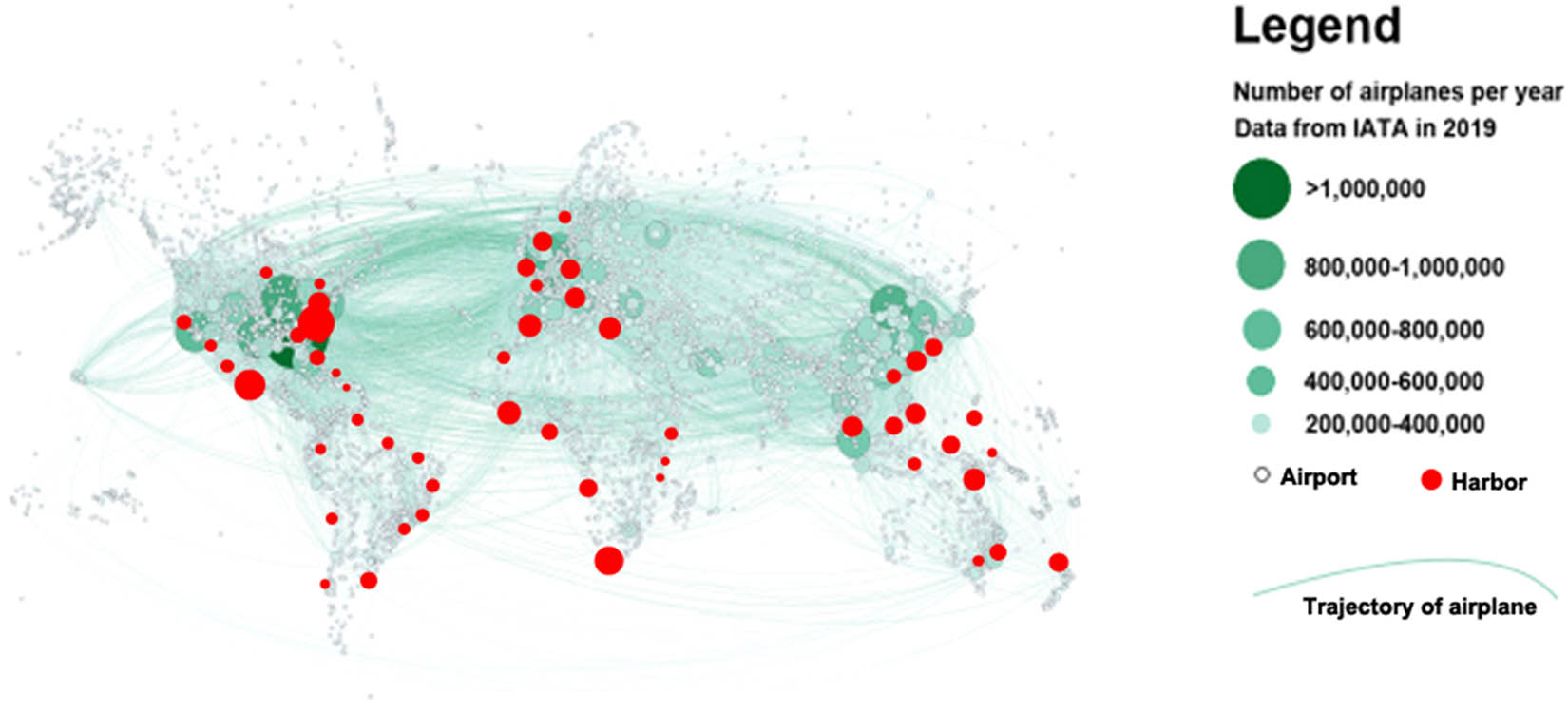
All airline routes in the world in 2019 with most connected harbors.
Using the methods of interpolation and buffer analysis, we obtained the belts which marked the length, i.e., the areas of 50, 100, and 200 km inland. The method of buffer analysis minimizes the estimation error. This way, the average population density is selected which gravitates around world harbors. In a similar way, using the methods of systematic GIS analysis, we obtained a complete image of 1,081 harbors connectivity with three modes of traffic and a population density that gravitates toward the coastlines. Finally, to test the the method in this work, the following procedures are introduced.
The first one concerns the determination of gravitational harbor nodes and their influence on geospace up to 50, 100, and 200 km. The second one is the determination of geographical position (geographical coordinates) concerning all the harbors examined and dealt with in this work. The third one is related to the determination of geographical azimuth and steep angle expressed in percentage. The geographical method with the help of GIS analysis has to show the general position of harbors in the world as well as their connectivity with means of transport up to 50, 100, and 200 km (see Figures 1–3).
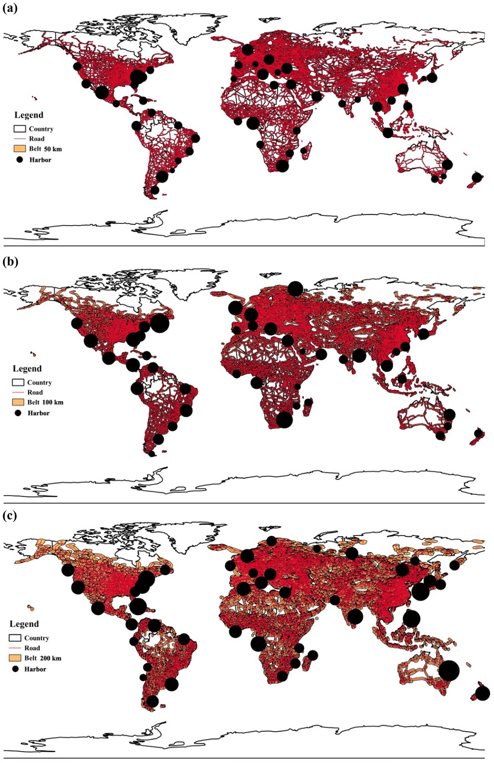
Road network and connect with harbors: (a) belt of the radius of 50 km, (b) belt of the radius of 100 km, and (c) the belt of the radius of 200 km.
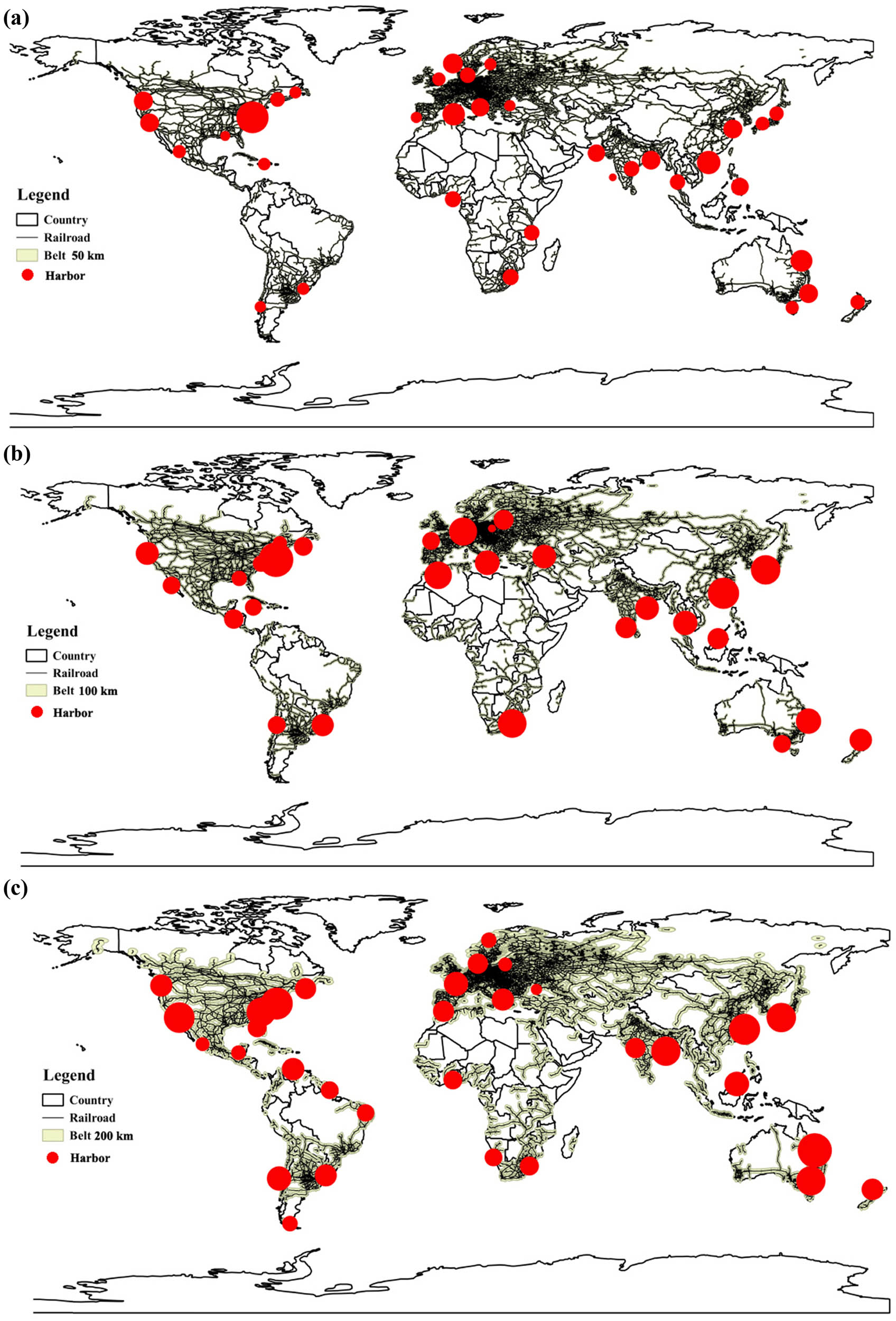
Railroad network and connect with harbors: (a) belt of the radius of 50 km, (b) belt of the radius of 100 km, and (c) the belt of the radius of 200 km.
2.1 GIS and numerical methods
In this research, GIS numerical methods have served as the basis for analyzing the position of harbors taken globally. Data modeling in the GIS environment represents a highly powerful tool for the calculation and analysis of harbor features all over the world. The position of harbors and their features are compared with the remaining modes of traffic using a precise GIS analysis. The method serving as support was the Interpolation Method. The software that served the purpose was SAGA. There are other procedures, algorithms, and methods which could be used for a similar purpose. The advantage of the Inverse Distance Algorithm is its minimization of error inside a spatial analysis. This means that the value may increase at a square distance. Due to the above-mentioned reasons, we have combined a multiple standard and untypical methods, so that when we calculate, we can reduce the errors to the minimum [27,28].
The analytics as well as the entire process is put into practice with the help of the open-source software. To determine the features and connectivity of railroad traffic as precisely as possible, in terms of their connectivity with marine harbors, the sophisticated Gephi 0.9.2. software has been used [29,30]. This software has a wide spectrum of possibilities since it reads 20 formats of mainly vector and compression extension. The nodes of all harbors as well as their networks (graphs) are decoded and analyzed by means of this software. In this software, all the available connecting linking points connected to the stream are analyzed to examine and analyze the accessibility of railroad and road hubs within the zones of 20, 50, and 100 km from the coast. With the help of advanced GIS and inside the QGIS software, we have initiated a highly precise algorithm or the function MMGIS. Inside the algorithm, it is possible to execute, along with the software Gephi 0.9, numerical analyses of high precision. The most important analysis carried out is proximity as well as semi-proximity, including the buffer classifying analysis that separates the results as belts. In total, after the demanding GIS and numerical, geo-static analysis, more complete data are obtained concerning the position values of world harbors [31].
3 Results and discussion
The results in this research show the maximum and minimum potential of traffic in comparison with harbors. The red spots present most connected harbors and airports. From Figure 1, we can see that the east coast of North America, west coast, north Europe, southern Europe, south-east Australia, a central part of Oceania, and south-east Africa have a good connection with harbors from the airplane traffic network; it can be seen that the total path length of all airplane lines in 2019 was 4.1 × 10¹⁵ km
The largest number of lines is between America and Europe (37%), then between Asia and Europe (33%), North America and South America (11%), Asia and East Asia (9%), Europe and Africa (5%), and others (5%). The total number of nodes (airports) is 5,623, and the total number of edges is 72,406. The results in modified Likert scale between airports and harbors are as follows: the mobility is 0.5; the connectivity is 0.4; the availability is 0.6; the density of graph which represents direct lines is 0.001; the modularity is 0.1; the average clustering coefficient is 0.270; and the centrality is 0.03 (see Table 1).
Properties of connection between Airplane network and harbors
| Continent | Centrality | Clustering coefficient | Modularity | Connectivity |
|---|---|---|---|---|
| Europe | 0.03 | 0.270 | 0.2 | Moderate |
| North America | 0.03 | 0.340 | 0.2 | Moderate |
| South America | 0.02 | 0.190 | 0.1 | Low |
| Asia | 0.03 | 0.330 | 0.2 | Moderate |
| Australia | 0.02 | 0.210 | 0.1 | Low |
| Africa | 0.01 | 0.190 | 0.1 | Low |
| Antarctica | 0.01 | 0.001 | 0.1 | Very low |
In USA, the biggest node is Atlanta’s airport, in Europe, the biggest nodes are identified in the UK (Heathrow), in Germany (Frankfurt Airport), in the Netherland (Schiphol), in France (Charles De Gaulle), and in Turkey (New International Airport). In Central Asia, the biggest nodes are (Sheremetyevo) in Russia (Beijing Capital International Airport) and (Shanghai Pudong International Airport) in China.
The densest road network is located in the eastern part of USA, western and central part of Europe, and east coast of China. The road traffic network between three continents, i.e., between North and South America across Central America is a closed network. The number of possible connected lines between main road nodes and harbors is 0.8 × 10⁹ per month (see Table 2). The roads of Europe, Asia, and Africa belong to the same closed network. The highest number of possible connected lines per month is in Europe 1.3 × 10⁸.
Properties of connection between road network and harbors
| Continent | Centrality | Clustering coefficient | Modularity | Connectivity |
|---|---|---|---|---|
| Europe | 0.05 | 0.430 | 0.6 | High |
| North America | 0.05 | 0.440 | 0.6 | High |
| South America | 0.03 | 0.310 | 0.4 | Moderate |
| Asia | 0.03 | 0.300 | 0.4 | Moderate |
| Australia | 0.02 | 0.280 | 0.3 | Moderate |
| Africa | 0.02 | 0.220 | 0.2 | Low |
| Antarctica | 0.00 | 0.000 | 0.1 | Very low |
The road networks in Australia and East Asia are isolated. The number of possible connected lines per month between harbors and road networks in Australia is 0.4 × 10⁷. In Asia, the number of possible connected lines per month is 1.2 × 10⁸. In South America, the number of possible connected lines per month is 0.6 × 10⁸ (see Table 2).
The railway traffic network has the following results: the mobility is 0.6; the connectivity is 0.3, and the availability is 0.8. The railway graph is relatively less connected in comparison with the road graph. The railway’s traffic network in North America represents the dependency graph. The number of possible connected lines per month between railroads and harbors is 1.3 × 10³.
The railway graph has the following characteristics: the average modularity is 0.3; the average clustering coefficient is 0.270; and the centrality is 0.04 (see Table 3).
Properties of connection between railroad network and harbors
| Continent | Centrality | Clustering coefficient | Modularity | Connectivity |
|---|---|---|---|---|
| Europe | 0.03 | 0.330 | 0.5 | High |
| North America | 0.03 | 0.310 | 0.5 | High |
| South America | 0.01 | 0.190 | 0.3 | Moderate |
| Asia | 0.02 | 0.220 | 0.3 | Low |
| Australia | 0.01 | 0.200 | 0.2 | Low |
| Africa | 0.01 | 0.280 | 0.2 | Low |
| Antarctica | 0.00 | 0.000 | 0.1 | Very low |
The number of possible connected lines per month in South America is 0.9 × 10². Europe has the largest railway network and the number of possible connected lines per month is 2.8 × 10³. In the railways of Asia, the number of possible connected lines per month is 0.9 × 10³ (see Table 3).
The results of the marine traffic network are as follows: the mobility is 0.2, the connectivity 0.1, and the availability 0.4. Harbors are highly distributed in Western Europe and the East of USA. GIS and numerical analysis have given the results related to the position of harbors and primary traffic features, i.e., mobility, connectivity, availability, density of connected lines, modularity, average clustering, and centrality. In total, the results of the whole 1,081 harbors are as follows: the mobility is 0.2; the connectivity is 0.1; the availability is 0.5, the density of connected lines, and the following ships (Cargo, Tankers, Tugs, Towing, Tugs-towing). The density of all the given lines according to the 2019 data is 0.0007 per square nautic mile (see Figure 4).
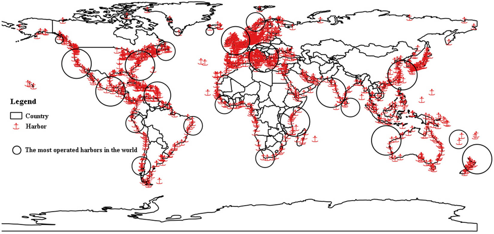
The distribution of the 1,081 harbors which used in this research with the most connected harbors.
The east coast of the United States of America has high connectivity and high potential of traffic flow with harbors. The following regions and countries exhibit similar results: Western Europe, South-east Europe, South East China, Japan, Central America, South Africa, South-east Australia, and all areas close to big agglomerations. The first belt with a radius of 50 km has high potential in the eastern parts of USA and Western Europe due to possible connectivity with other types of traffic. The belt of 100 km covers the same areas. Finally, the belt of 200 km radius covers 75% of the total connection with harbors.
According to the 2019 situation, the highest density is in the regions of Northern India, Central, and Western Europe, as well as the east coast of USA. The harbors are highly distributed in Western Europe and the East of USA. The remaining regions with a big population density are eastern China, eastern and south-east Australia, the Japanese archipelago, big agglomerations in Africa and South America. In these regions, the population density is 100 inhabitants per square kilometer. On average, these areas are 250 km distant from the major harbors. Only 15% of densely populated areas (100 inhabitants per square kilometer) are 100 km distant from the coastline. The biggest megalopolises in the world such as Tokyo (Japan), Delhi (India), Shanghai (China), Sao Paolo (Brazil), Mexico City (Mexico), Dhaka (Bangladesh), Cairo (Egypt), Beijing (China), Mumbai (India), Osaka (Japan), Karachi (Pakistan), Chongqing (China), Istanbul (Turkey), Buenos Aries (Argentina), Kolkata (India), Logos (Nigeria), Kinshasa (Congo), Manila (Philippines), Tianjin (China), and Rio De Janeiro (Brazil) have a density between 500 and 1,000 inhabitants per square kilometer. These most highly populated areas on the planet are, in average terms, 70 km away from the major world harbors and 90% are inside the belt of 100 km. Thus, the most densely populated areas are well connected with major harbors. This fact indicates changes that will occur in the future when urbanization and city expansion are concerned. More than 387,000,000 inhabitants gravitate within the best connectivity with major world sea harbors. On doing a GIS analysis according to the current UN prediction, we have calculated that more than 70% of the population will live at a distance less than 50 km away from world harbors (see Figure 5).
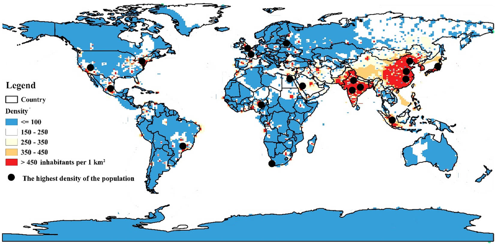
The density of population on a global scale.
After doing a GIS analysis, almost all sea harbors of the world show a good connection, apart from those which are on isolated islands and which are at the geographical latitude above 70°N I 70°S. If we expect the melting of ice after climate change, the good connectivity will have harbors on Greenland and Antarctica. Speaking of railroad connections, the densest network is by all means in western and central Europe. In one part of the United States as well as in Eastern Asia, on carrying out a GIS software analysis, we have concluded that 30% of railroad communications has a good connection with sea harbors taken globally. The countries with exceptional sea potentials due to their geographical positions are Mexico, Panama, and Cuba in Central America, Chile, Brazil, and Argentina in South America. The countries with the highest number of ports (nodes) are the United Kingdom, France, Italy, Spain, Greece, Turkey, Russia, Denmark, Norway, Finland, Ireland, and Island. In North America, the east coast has more ports than the west coast; Morocco, Egypt, and Algeria in North Africa; Angola and Nigeria in West Africa; the South African Republic in South Africa; Madagascar and Kenya in East Africa; and China, Indonesia, Saudi Arabia, Iran, Filipinas, South Korea, Japan, and the Asian part of the Russian Federation in Asia (Figure 5).
Regardless of the traffic mobility being low, the possibility of carrying a huge cargo as well as the notable presence of the population that will gravitate toward the harbor might be a huge advantage. GIS and geographical analysis, in this research, have shown that 70% of harbors have a good connectivity with regional and international roads. About 20% of the harbors have the best possible connectivity with railroad nodes. The best connectivity is with European harbors, harbors in the United States and southeast Asia, which includes all types of traffic. About 12% is extremely low connected, 62% displays medium connectivity, whereas 26% displays excellent connectivity. About 80% of the well-connected harbors with all modes of traffic belong to Asia, 10% to North America, and 10% to Europe. On carrying out the analyses, European harbors have the best connectivity with railroad nodes and the North American ones with roads. This research has shown that Africa, due to its prominent geographical position, has the biggest potential in the further development and the opening of sea harbors. The research has taken into consideration the geographical position of 1,081 harbors, their dispersion as well as their connectivity with all modes of traffic 200 km long. American east coast has the best connectivity up to 50 km, as well as harbors in South East Asia. Central American and Western American harbors have a connection; in South Africa, it is 0–50 km. In Eastern Australia and South Asia, the belt stretches to 50 km as well as in South America. North and East African harbors have an average distance of 100–200 km. Antarctic harbors as those on isolated islands are least connected with the network of all the three traffic modes whose distance exceeds 200 km. The buffer and interpolation models outline that GIS techniques, resources, and methods can be efficiently used for more effective investigation of geographical locations of harbors in the world (see Figure 4).
After finished buffer analysis, we have data and calculations for buffer zones in comparison with the positions of harbors. The most useful areas in the future are zones on the east coast in the United States, zones in the California Bay harbor on the west coast in the United States on the Pacific side, and zones of the east coast in USA. In the future, valuable geographic positions are situated in Mexico and Panama, westside of South America, and eastside of Chile and south part of Argentina. Europe has good potential in connecting harbors even in Scandinavia: in Africa, south parts of Africa, Madagascar, East Africa, Bay of Guinea, Durban, and Madagascar and in Asia, Persian Gulf, Gulf of Thailand, South China Sea, Bay Bengal, east part of Japan, western Australia, and southeast Australia. The road connection has 56% better connection than railroads with harbors on a global scale. The railroads at a global scale depend on low connectivity with the main harbors. Hence, we calculated that railroads have 35% fewer networks to the harbors than road networks. The main zones are the Gulf of Alaska, California, Gulf of Mexico, Florida, Philadelphia, New York, and Nova Scotia; in South America, Sao Paolo and Montevideo; in Africa, Cape Town and Durban; in Europe, we have a better connection almost with all harbors; in Asia, Mumbai, Calcutta, Hong Kong, east coast of China, Japan, Vladivostok. In Australia Melbourne, Sydney, and Brisbane.
4 Conclusion
GIS and the geographical analysis of the 1,081 biggest harbors in the world have shown their position and potential in relation to all modes of traffic within 200 km off the coast. Major traffic features such as connectivity, mobility, availability, centrality, and clustering coefficient have shown all the advantages and flaws of road, railroad, and marine traffic. All three types of traffic are compared with the order and position of sea harbors. In this paper, it was noted that air traffic in the future has numerous new airports and because of that a high possibility for mobility, especially in USA and Europe, as well as in Mainland China. The road traffic has good possibility in connection with harbors in 80% of the territories. The connectivity of harbors with other traffic networks is ranked as average – it is better with the road traffic system and less for 30% with railway traffic. The reason for this lies in the fact that the speed of air traffic is relatively high, and a number of new. Road traffic has high mobility, the highest connectivity, and reliable availability.
Advanced GIS methods as well as geographical analyses have displayed the weaknesses and advantages of the current harbor positions as well as their future potentials. The seven continents, including the Antarctic, have been included in the study. GIS methods such as clustering, buffer, zonality, kriging, and interpolation have helped in terms of better isolation and the characteristics of harbors themselves globally. This analysis has shown that old sea harbors are still important and that they are very well connected with traffic hubs. The analysis of harbors in relation to general population density, finalized with the 2019 situation, showed that world harbors were near great agglomerations, which might appear both as an advantage and a disadvantage. The advantage lies in a better industrial accessibility, including traffic and population, while the disadvantage is in the potential overburdening of traffic infrastructure in the future. The solution to the problem may be the opening of new harbors, along with the existing old ones, as well as the rebuilding of new traffic connections for the sake of better accessibility. The analysis has shown that Europe, the east coast of America, and southeast Asia are still main nodes, being solidly bound especially with road communications. The rest of the continents are less connected yet with the potentials that could be better in the future by building new communications. Africa, being a central continent with a good geographical position, might in the future, especially with its western part, become a major marine node having new harbors built. This work may represent a solid basis for further research related to world harbors. Other analysis, apart from GIS and geographical ones, would be a good foundation for creating a detailed analysis which besides this one would be a basis for further marine traffic development.
Finally, we know that this research has some limitations and disadvantages, but it would be good to extend with some new and different approaches. Regardless of everything, this research would be important for all spatial science, marine investigation, and geography. The buffer zones in this research showed that roads have a better possibility of connecting than railroads, especially in belts of 200 km from harbors. Good harbors must have an equal relationship between the density of population, commodity, and real necessity of marine traffic. This research in the future may be extended with a new database that is better connected on a local and regional scale.
Acknowledgment
The authors are grateful to the anonymous reviewers whose constructive comments and suggestions greatly improved the manuscript. Serbian Ministry of Education and Science is supported this work within the projects No III44006 and No III43007.
-
Author contribution: AV had the original idea for the manuscript and created all maps. AV, SŠ, and JG gave the methodology; DR, NB, NM, MI, created the tables, all authors organized and analyzed traffic data and structure of the manuscript.
-
Conflict of interest: Authors state no conflict of interest.
References
[1] Goss R. An early history of maritime economics. Int J Marit Econ. 2002;4:390–404. 10.1057/palgrave.ijme.9100052.Search in Google Scholar
[2] Jung PH, Kashiha M, Thill JC. Community structures in networks of disaggregated cargo flows to maritime ports. In: Popovich V, Schrenk M, Thill JC, Claramunt C, Wang T, editors. Information fusion and intelligent geographic information systems (IF&IGIS’17). Lecture notes in geoinformation and cartography. Cham: Springer; 2018. 10.1007/978-3-319-59539-9_13.Search in Google Scholar
[3] Fujita M, Tomoya M. The role of ports in the making of major cities: self-agglomeration and hub-effect. J Dev Econ. 1996;49(1):93–120. 10.1016/0304-3878(95)00054-2.Search in Google Scholar
[4] Carpenter A, Lozano R. Proposing a framework for anchoring sustainability relationships between ports and cities. In: Carpenter A, Lozano R, editors. European port cities in transition strategies for sustainability. Cham: Springer; 2020. 10.1007/978-3-030-36464-9_3.Search in Google Scholar
[5] Luan W, Chen H, Wang Y. Simulating mechanism of interaction between ports and cities based on system dynamics: a case of Dalian, China. Chin Geogr Sci. 2010;20:398–405. 10.1007/s11769-010-0413-5.Search in Google Scholar
[6] Noble M, Harasti D, Pittock J, Doran B. Linking the social to the ecological using GIS methods in marine spatial planning and management to support resilience: a review. Mar Policy. 2019;108:103657. 10.1007/s12517-011-0394-4.Search in Google Scholar
[7] Cohen P, Monaco K. Inter-county spillovers in California’s ports and roads infrastructure: the impact on retail trade. Lett Spat Resour Sci. 2009;2:77. 10.1007/s12076-009-0025-9.Search in Google Scholar
[8] Joseph M, Wang F. Population density patterns in Port-au-Prince, Haiti: a model of Latin American city? Cities. 2010;27(3):127–36. 10.1016/j.cities.2009.12.002.Search in Google Scholar
[9] Small C, Nicholls R. A global analysis of human settlement in coastal zones. J Coast Res. 2003;19(3):584–99.Search in Google Scholar
[10] Hu S, Zhang J. Risk assessment of marine traffic safety at coastal water area. Procedia Eng. 2012;45:31–7. 10.1016/j.proeng.2012.08.116.Search in Google Scholar
[11] Hashimoto A, Okushima T. Evaluating marine traffic safety at channels. Accid Anal Prev. 1990;22(5):421–42. 10.1016/0001-4575(90)90038-M.Search in Google Scholar
[12] De Langen W. Chapter 20 stakeholders, conflicting interests and governance in port clusters. Res Transport Econ. 2006;17:457–77.10.1016/S0739-8859(06)17020-1Search in Google Scholar
[13] Notteboom T. From multi-porting to a hub port configuration: the South African container port system in transition. Int J Shipping Transp Logist. 2010;2(2):224–45. 10.1504/IJSTL.2010.030868.Search in Google Scholar
[14] Silveira P, Teixeira A, Soares C. Use of AIS data to characterise marine traffic patterns and ship collision risk off the coast of Portugal. J Navigation. 2013;66(6):879–98. 10.1017/S037346331300051.Search in Google Scholar
[15] Ducruet C, Joly O, Le Cam M. Europe in global maritime flows: gateways, forelands and subnetworks. Changing urban and regional relations in a globalizing World Europe as a global macro-region. United Kingdom: Edward Elgar Publishing Limited; 2014. p. 164–80.10.4337/9781782544654.00016Search in Google Scholar
[16] Lotze K, Chénier R, Abado L, Sabourin O, Tardif L. Northern marine transportation corridors: creation and analysis of northern marine traffic routes in Canadian waters. Transit GIS. 2017;21(6):1085–97. 10.1111/tgis.12295.Search in Google Scholar
[17] Lasserrea F, Pelletierb S. Polar super seaways? Maritime transport in the Arctic: an analysis of shipowners’ intentions. J Transp Geogr. 2011;19(6):1465–73. 10.1016/j.jtrangeo.2011.08.006.Search in Google Scholar
[18] Lutz W, Sanderson W, Scherbov S. The end of world population growth. Nature. 2001;412:543–5. 10.1038/35087589.Search in Google Scholar PubMed
[19] Wang Z, Claramunt C, Wang Y. Extracting global shipping networks from massive historical automatic identification system sensor data: a bottom-up approach. Sensors. 2019;19(15):3363. 10.3390/s19153363.Search in Google Scholar PubMed PubMed Central
[20] https://www.marinetraffic.com/en/ais/home/centerx:-12.0/centery:25.0/zoom:4. Accessed on 05.07.2020.Search in Google Scholar
[21] Sullivan MA. Analyzing and interpreting data from likert-type scales. J Graduate Med Educ. 2013;5:541–2.10.4300/JGME-5-4-18Search in Google Scholar PubMed PubMed Central
[22] Aydogdu Y, Yurtoren C, Park J, Park YA. Study on local traffic management to improve marine traffic safety in the Istanbul strait. J Navigation. 2012;65(1):99–112. 10.1017/S0373463311000555.Search in Google Scholar
[23] Robinson A, Morrison J, Muehrcke P, Kimerling J, Guptill S. Elements of cartography. 6th ed. Ottawa, Canada: John Willey and Sons; 1995.Search in Google Scholar
[24] Wright K. Crossbreeding geographical quantiles. Geograph Rev. 1995;45:52–65.10.2307/211729Search in Google Scholar
[25] Nykiforuk C, Flaman L. Geographic information systems (GIS) for health promotion and public health: a review. Health Promot Pract. 2011;12(1):63–73. 10.1177/1524839909334624.Search in Google Scholar PubMed
[26] Wu S, Chen Y. Examining eco-environmental changes at major recreational sites in Kenting National Park in Taiwan by integrating SPOT satellite images and NDVI. Tour Manag. 2016;57:23–36. 10.1016/j.tourman.2016.05.006.Search in Google Scholar
[27] Valjarević A, Djekić T, Stevanović V, Ivanović R, Jandziković B. GIS numerical and remote sensing analyses of forest changes in the Toplica region for the period of 1953–2013. Appl Geogr. 2018;92:131–9. 10.1016/j.apgeog.2018.01.016.Search in Google Scholar
[28] Valjarević A, Filipović D, Milanović M, Valjarević D. New updated World maps of sea-surface salinity. Pure Appl Geophys. 2020;177:2977–92. 10.1007/s00024-019-02404-z.Search in Google Scholar
[29] Guo D. Visual analytics of spatial interaction patterns for pandemic decision support. Int J Geograph Inf Sci. 2007;21(8):859–77. 10.1080/13658810701349037.Search in Google Scholar
[30] Zhou C, Su F, Pei T, Zhang A, Du Y, Luo B, et al. COVID-19: challenges to GIS with big data. Geogr Sustain. 2020;1:77–87. 10.1016/j.geosus.2020.03.005.Search in Google Scholar
[31] Han X, Naeher L. A review of traffic-related air pollution exposure assessment studies in the developing world. Environ Int. 2006;32:106–20. 10.1016/j.envint.2005.05.020.Search in Google Scholar PubMed
© 2021 Aleksandar Valjarević et al., published by De Gruyter
This work is licensed under the Creative Commons Attribution 4.0 International License.
Articles in the same Issue
- Regular Articles
- Lithopetrographic and geochemical features of the Saalian tills in the Szczerców outcrop (Poland) in various deformation settings
- Spatiotemporal change of land use for deceased in Beijing since the mid-twentieth century
- Geomorphological immaturity as a factor conditioning the dynamics of channel processes in Rządza River
- Modeling of dense well block point bar architecture based on geological vector information: A case study of the third member of Quantou Formation in Songliao Basin
- Predicting the gas resource potential in reservoir C-sand interval of Lower Goru Formation, Middle Indus Basin, Pakistan
- Study on the viscoelastic–viscoplastic model of layered siltstone using creep test and RBF neural network
- Assessment of Chlorophyll-a concentration from Sentinel-3 satellite images at the Mediterranean Sea using CMEMS open source in situ data
- Spatiotemporal evolution of single sandbodies controlled by allocyclicity and autocyclicity in the shallow-water braided river delta front of an open lacustrine basin
- Research and application of seismic porosity inversion method for carbonate reservoir based on Gassmann’s equation
- Impulse noise treatment in magnetotelluric inversion
- Application of multivariate regression on magnetic data to determine further drilling site for iron exploration
- Comparative application of photogrammetry, handmapping and android smartphone for geotechnical mapping and slope stability analysis
- Geochemistry of the black rock series of lower Cambrian Qiongzhusi Formation, SW Yangtze Block, China: Reconstruction of sedimentary and tectonic environments
- The timing of Barleik Formation and its implication for the Devonian tectonic evolution of Western Junggar, NW China
- Risk assessment of geological disasters in Nyingchi, Tibet
- Effect of microbial combination with organic fertilizer on Elymus dahuricus
- An OGC web service geospatial data semantic similarity model for improving geospatial service discovery
- Subsurface structure investigation of the United Arab Emirates using gravity data
- Shallow geophysical and hydrological investigations to identify groundwater contamination in Wadi Bani Malik dam area Jeddah, Saudi Arabia
- Consideration of hyperspectral data in intraspecific variation (spectrotaxonomy) in Prosopis juliflora (Sw.) DC, Saudi Arabia
- Characteristics and evaluation of the Upper Paleozoic source rocks in the Southern North China Basin
- Geospatial assessment of wetland soils for rice production in Ajibode using geospatial techniques
- Input/output inconsistencies of daily evapotranspiration conducted empirically using remote sensing data in arid environments
- Geotechnical profiling of a surface mine waste dump using 2D Wenner–Schlumberger configuration
- Forest cover assessment using remote-sensing techniques in Crete Island, Greece
- Stability of an abandoned siderite mine: A case study in northern Spain
- Assessment of the SWAT model in simulating watersheds in arid regions: Case study of the Yarmouk River Basin (Jordan)
- The spatial distribution characteristics of Nb–Ta of mafic rocks in subduction zones
- Comparison of hydrological model ensemble forecasting based on multiple members and ensemble methods
- Extraction of fractional vegetation cover in arid desert area based on Chinese GF-6 satellite
- Detection and modeling of soil salinity variations in arid lands using remote sensing data
- Monitoring and simulating the distribution of phytoplankton in constructed wetlands based on SPOT 6 images
- Is there an equality in the spatial distribution of urban vitality: A case study of Wuhan in China
- Considering the geological significance in data preprocessing and improving the prediction accuracy of hot springs by deep learning
- Comparing LiDAR and SfM digital surface models for three land cover types
- East Asian monsoon during the past 10,000 years recorded by grain size of Yangtze River delta
- Influence of diagenetic features on petrophysical properties of fine-grained rocks of Oligocene strata in the Lower Indus Basin, Pakistan
- Impact of wall movements on the location of passive Earth thrust
- Ecological risk assessment of toxic metal pollution in the industrial zone on the northern slope of the East Tianshan Mountains in Xinjiang, NW China
- Seasonal color matching method of ornamental plants in urban landscape construction
- Influence of interbedded rock association and fracture characteristics on gas accumulation in the lower Silurian Shiniulan formation, Northern Guizhou Province
- Spatiotemporal variation in groundwater level within the Manas River Basin, Northwest China: Relative impacts of natural and human factors
- GIS and geographical analysis of the main harbors in the world
- Laboratory test and numerical simulation of composite geomembrane leakage in plain reservoir
- Structural deformation characteristics of the Lower Yangtze area in South China and its structural physical simulation experiments
- Analysis on vegetation cover changes and the driving factors in the mid-lower reaches of Hanjiang River Basin between 2001 and 2015
- Extraction of road boundary from MLS data using laser scanner ground trajectory
- Research on the improvement of single tree segmentation algorithm based on airborne LiDAR point cloud
- Research on the conservation and sustainable development strategies of modern historical heritage in the Dabie Mountains based on GIS
- Cenozoic paleostress field of tectonic evolution in Qaidam Basin, northern Tibet
- Sedimentary facies, stratigraphy, and depositional environments of the Ecca Group, Karoo Supergroup in the Eastern Cape Province of South Africa
- Water deep mapping from HJ-1B satellite data by a deep network model in the sea area of Pearl River Estuary, China
- Identifying the density of grassland fire points with kernel density estimation based on spatial distribution characteristics
- A machine learning-driven stochastic simulation of underground sulfide distribution with multiple constraints
- Origin of the low-medium temperature hot springs around Nanjing, China
- LCBRG: A lane-level road cluster mining algorithm with bidirectional region growing
- Constructing 3D geological models based on large-scale geological maps
- Crops planting structure and karst rocky desertification analysis by Sentinel-1 data
- Physical, geochemical, and clay mineralogical properties of unstable soil slopes in the Cameron Highlands
- Estimation of total groundwater reserves and delineation of weathered/fault zones for aquifer potential: A case study from the Federal District of Brazil
- Characteristic and paleoenvironment significance of microbially induced sedimentary structures (MISS) in terrestrial facies across P-T boundary in Western Henan Province, North China
- Experimental study on the behavior of MSE wall having full-height rigid facing and segmental panel-type wall facing
- Prediction of total landslide volume in watershed scale under rainfall events using a probability model
- Toward rainfall prediction by machine learning in Perfume River Basin, Thua Thien Hue Province, Vietnam
- A PLSR model to predict soil salinity using Sentinel-2 MSI data
- Compressive strength and thermal properties of sand–bentonite mixture
- Age of the lower Cambrian Vanadium deposit, East Guizhou, South China: Evidences from age of tuff and carbon isotope analysis along the Bagong section
- Identification and logging evaluation of poor reservoirs in X Oilfield
- Geothermal resource potential assessment of Erdaobaihe, Changbaishan volcanic field: Constraints from geophysics
- Geochemical and petrographic characteristics of sediments along the transboundary (Kenya–Tanzania) Umba River as indicators of provenance and weathering
- Production of a homogeneous seismic catalog based on machine learning for northeast Egypt
- Analysis of transport path and source distribution of winter air pollution in Shenyang
- Triaxial creep tests of glacitectonically disturbed stiff clay – structural, strength, and slope stability aspects
- Effect of groundwater fluctuation, construction, and retaining system on slope stability of Avas Hill in Hungary
- Spatial modeling of ground subsidence susceptibility along Al-Shamal train pathway in Saudi Arabia
- Pore throat characteristics of tight reservoirs by a combined mercury method: A case study of the member 2 of Xujiahe Formation in Yingshan gasfield, North Sichuan Basin
- Geochemistry of the mudrocks and sandstones from the Bredasdorp Basin, offshore South Africa: Implications for tectonic provenance and paleoweathering
- Apriori association rule and K-means clustering algorithms for interpretation of pre-event landslide areas and landslide inventory mapping
- Lithology classification of volcanic rocks based on conventional logging data of machine learning: A case study of the eastern depression of Liaohe oil field
- Sequence stratigraphy and coal accumulation model of the Taiyuan Formation in the Tashan Mine, Datong Basin, China
- Influence of thick soft superficial layers of seabed on ground motion and its treatment suggestions for site response analysis
- Monitoring the spatiotemporal dynamics of surface water body of the Xiaolangdi Reservoir using Landsat-5/7/8 imagery and Google Earth Engine
- Research on the traditional zoning, evolution, and integrated conservation of village cultural landscapes based on “production-living-ecology spaces” – A case study of villages in Meicheng, Guangdong, China
- A prediction method for water enrichment in aquifer based on GIS and coupled AHP–entropy model
- Earthflow reactivation assessment by multichannel analysis of surface waves and electrical resistivity tomography: A case study
- Geologic structures associated with gold mineralization in the Kirk Range area in Southern Malawi
- Research on the impact of expressway on its peripheral land use in Hunan Province, China
- Concentrations of heavy metals in PM2.5 and health risk assessment around Chinese New Year in Dalian, China
- Origin of carbonate cements in deep sandstone reservoirs and its significance for hydrocarbon indication: A case of Shahejie Formation in Dongying Sag
- Coupling the K-nearest neighbors and locally weighted linear regression with ensemble Kalman filter for data-driven data assimilation
- Multihazard susceptibility assessment: A case study – Municipality of Štrpce (Southern Serbia)
- A full-view scenario model for urban waterlogging response in a big data environment
- Elemental geochemistry of the Middle Jurassic shales in the northern Qaidam Basin, northwestern China: Constraints for tectonics and paleoclimate
- Geometric similarity of the twin collapsed glaciers in the west Tibet
- Improved gas sand facies classification and enhanced reservoir description based on calibrated rock physics modelling: A case study
- Utilization of dolerite waste powder for improving geotechnical parameters of compacted clay soil
- Geochemical characterization of the source rock intervals, Beni-Suef Basin, West Nile Valley, Egypt
- Satellite-based evaluation of temporal change in cultivated land in Southern Punjab (Multan region) through dynamics of vegetation and land surface temperature
- Ground motion of the Ms7.0 Jiuzhaigou earthquake
- Shale types and sedimentary environments of the Upper Ordovician Wufeng Formation-Member 1 of the Lower Silurian Longmaxi Formation in western Hubei Province, China
- An era of Sentinels in flood management: Potential of Sentinel-1, -2, and -3 satellites for effective flood management
- Water quality assessment and spatial–temporal variation analysis in Erhai lake, southwest China
- Dynamic analysis of particulate pollution in haze in Harbin city, Northeast China
- Comparison of statistical and analytical hierarchy process methods on flood susceptibility mapping: In a case study of the Lake Tana sub-basin in northwestern Ethiopia
- Performance comparison of the wavenumber and spatial domain techniques for mapping basement reliefs from gravity data
- Spatiotemporal evolution of ecological environment quality in arid areas based on the remote sensing ecological distance index: A case study of Yuyang district in Yulin city, China
- Petrogenesis and tectonic significance of the Mengjiaping beschtauite in the southern Taihang mountains
- Review Articles
- The significance of scanning electron microscopy (SEM) analysis on the microstructure of improved clay: An overview
- A review of some nonexplosive alternative methods to conventional rock blasting
- Retrieval of digital elevation models from Sentinel-1 radar data – open applications, techniques, and limitations
- A review of genetic classification and characteristics of soil cracks
- Potential CO2 forcing and Asian summer monsoon precipitation trends during the last 2,000 years
- Erratum
- Erratum to “Calibration of the depth invariant algorithm to monitor the tidal action of Rabigh City at the Red Sea Coast, Saudi Arabia”
- Rapid Communication
- Individual tree detection using UAV-lidar and UAV-SfM data: A tutorial for beginners
- Technical Note
- Construction and application of the 3D geo-hazard monitoring and early warning platform
- Enhancing the success of new dams implantation under semi-arid climate, based on a multicriteria analysis approach: Case of Marrakech region (Central Morocco)
- TRANSFORMATION OF TRADITIONAL CULTURAL LANDSCAPES - Koper 2019
- The “changing actor” and the transformation of landscapes