Constructing 3D geological models based on large-scale geological maps

Xuechao Wu; Gang Liu; Zhengping Weng; Yiping Tian; Zhiting Zhang; Yang Li; Genshen Chen

doi:10.1515/geo-2020-0270

Artikel Open Access

Constructing 3D geological models based on large-scale geological maps

Xuechao Wu , Gang Liu , Zhengping Weng , Yiping Tian , Zhiting Zhang , Yang Li und Genshen Chen

Veröffentlicht/Copyright: 9. August 2021

Veröffentlicht von

Veröffentlichen auch Sie bei De Gruyter Brill

Manuskript einreichen Informationen für Autor*innen

Aus der Zeitschrift Open Geosciences Band 13 Heft 1

Abstract

The construction of 3D geological models based on geological maps is a subject worthy of study. The construction of geological interfaces is the key process of 3D geological modeling. It is hard to build the bottom interfaces of quaternary strata only using boundaries in large-scale geological maps. Moreover, it is impossible to construct bedrock geological interfaces through sparse occurrence data in large-scale geological maps. To address the above-mentioned two difficulties, we integrated two key algorithms into a new 3D modeling workflow. The buffer algorithm was used to construct virtual thickness contours of quaternary strata. The Inverse Distance Weighted (IDW) algorithm was applied to occurrence interpolation. Using a regional geological map of a city in southern China, the effectiveness of our workflow was verified. The complex spatial geometry of quaternary bottom interfaces was described in detail through boundaries buffer. The extension trends of bedrock geological interfaces were reasonably constraint by occurrence interpolation. The 3D geological model constructed by our workflow accords with the semantic relationship of tectonics. Through the model, the complex spatial structure of urban shallow strata can be displayed stereoscopically. It can provide auxiliary basis for decision-making of urban underground engineering.

Keywords: 3D geological modeling; large-scale geological maps; geological interfaces; virtual thickness contours; occurrence interpolation

1 Introduction

3D geological modeling technology is the basic and supporting technology of many major research projects. 3D visualization of underground space can provide a more real and intuitive description of geological phenomena and structures [1,2]. In recent years, with the rapid development of urbanization, geological problems have become increasingly prominent. 3D geological models can not only describe underground geological information accurately, but also provide decision basis for urban resource analysis, underground engineering planning, and disaster prevention and reduction [3,4,5]. Urban underground 3D geological modeling has become an important topic in smart city research [6,7].

The existing 3D geological modeling methods are mainly based on underground data such as boreholes, sections, geophysical data, and integrated multisource data. Jiskani et al. built a 3D modeling of multiple coal seams effectively through drilling data [8]. Zhu et al. used an automatic method to build 3D solid models of sedimentary stratigraphic systems from borehole data [9]. Chen et al. proposed a locality-based MPS approach to reconstruct 3D geological models on the basis of 2D cross sections [10]. Wang et al. constructed the 3D geological model of Luanchuan ore region by combining geological knowledge with gravitational and magnetic data inversion [11]. Kaufmann and Martin presented a 3D modeling method by integrating boreholes, outcrops, cross sections, and geological maps and it has been well-applied in coal mines [12]. Qiao et al. proposed an approach to establish 3D strata model from DEM, borehole, section map, and geological map and the fast update of strata model can be realized with the new redefined cross section [13]. The 3D geological models established by underground data are relatively fine and accurate. However, due to the restriction of economy and other conditions, it is difficult to deploy enough underground projects in cities for exploration. As a result, these underground exploration data are very sparse or even absent in urban areas. Therefore, the 3D geological models of cities can hardly be constructed by sparse underground data. In this case, we need a kind of data which can support modeling and are easy to obtain. Geological maps are the main achievements of regional geological survey. They are produced by projecting various field geological survey data on topographic base map in a certain proportion. They contain a wealth of geological knowledge inferred from field survey data by geological experts. Moreover, they are a kind of data which are cheap and relatively easy to obtain [14]. Through geological maps, we can know the topography, lithology, occurrence data, the nature, and spatial distribution form of geological structures of an area directly [15]. After the analysis, geological maps can reveal the contact relationships between strata and strata, strata and structures, and structures and structures, which are incomparable with boreholes and sections [16]. What’s more, the occurrence data in geological maps can also reveal the extension trend of geological interfaces in the underground shallow strata [17]. Therefore, under the premise of lacking other geological data, the idea of constructing 3D geological framework models of shallow strata by using geological maps is feasible in theory.

In view of the above background, more and more scholars begin to pay attention to and study the 3D geological modeling method based on geological maps. Amorim et al. used sketches and annotations from geological maps to construct 3D geological models [18]. The annotations mainly refer to the occurrence information of strata. Under the constraint of occurrence data, the Hermite–Birkhoff Radial Basis function (HBRBF) was applied to construct implicit geological interfaces. Guo et al. used geological boundaries and attitudes from geological maps to construct 3D geological models [19]. Attitude is described by dip direction and dip angle. Under the constraint of attitudes, the geological boundaries were used to construct the implicit geological interfaces using the Hermite Radial Basis Function (HRBF) [20,21,22]. Zhou et al. proposed a 3D geological modeling method based on planar geological maps [23]. Under the control of occurrence data, a series of parallel map-cut-sections can be automatically drawn. The geological boundaries and parallel map-cut-sections were combined to constrain and reconstruct the geological interfaces. Lin et al. presented a method for constructing a detail 3D model from 2D geological maps [24]. A series of cross map-cut-sections were created with the help of occurrence data in geological maps. The geological boundaries and cross map-cut-sections were combined to construct geological interfaces. Zhang et al. constructed a 3D geological model of metallogenic geological bodies based on a planar geological map [25]. A series of parallel map-cut-sections were constructed with the participation of occurrence data. The geological boundaries on the geological map and outlines in parallel map-cut-sections were combined to reconstruct geological interfaces.

According to the above methods, the core work of establishing 3D geological models with geological maps is the construction of geological interfaces. The geological maps they have used are small-scale. In small-scale geological maps, there is no complex quaternary and the occurrence data are relatively complete. Therefore, they can construct geological interfaces successfully through implicit surface construction method or map-cut-sections method. In this paper, we discuss the construction of 3D geological models based on large-scale geological maps. Large-scale geological maps usually contain extensive quaternary characterized by complex morphology, uneven distribution, and thin thickness [26]. The occurrence data of bedrock in large-scale geological maps are often very sparse. So there are two main difficulties in constructing geological interfaces based on large-scale geological maps. First, it is difficult to construct quaternary bottom interfaces only depending on boundaries. The reason is that there is no other underground data to constrain the extremely complex morphology of quaternary bottom interfaces. Second, bedrock geological interfaces cannot be constructed only by sparse occurrence data. The reason is that the sparse occurrence data can not constrain the extension of bedrock geological interfaces in the underground.

The main purpose of this work is to put forward an effective 3D modeling workflow based on large-scale geological maps. This workflow will apply two key algorithms to solve the above two difficulties. The internal buffer algorithm of closed lines will creatively adopt to generate virtual thickness contours of quaternary overburden. The virtual thickness contours will be used to construct the bottom interfaces of quaternary strata with complex morphology. The Inverse Distance Weighted (IDW) algorithm will be used to interpolate the occurrence information of the control points on the bedrock geological boundaries. Through the occurrence interpolation, we will have enough occurrence information to reasonably constrain the extension of bedrock interfaces in the underground. In order to verify the effectiveness of this workflow, a large-scale geological map will be used to construct a 3D geological framework model of a city in southern China. The geological model can provide auxiliary basis for decision-making of urban underground engineering.

2 Modeling workflow

In the absence of boreholes, sections, and geophysical data, we propose a new modeling workflow to build 3D geological framework models of shallow strata by using large-scale geological maps (Figure 1). This workflow mainly includes the data organization of geological maps, the integration of two key algorithms and the construction of geological interfaces, and the extraction of geological bodies.

Figure 1

Modeling workflow based on large-scale geological maps.

The 3D geological modeling units are the geological bodies separated by the geological interfaces, so the construction of geological interfaces is a key link in the workflow of 3D geological modeling. Therefore, we will focus on the methods of constructing geological interfaces of different geological units.

2.1 Construction of quaternary bottom interfaces

The geological boundaries and average thickness of quaternary overburden can be obtained from geological maps. Referring to the idea of drawing strata planar thickness contour map, the planar virtual thickness contours of quaternary overburden can be constructed by using the internal buffer algorithm of closed lines. According to the corresponding thickness value, the planar virtual thickness contours can be sunk into 3D space to form the 3D virtual thickness contours. Finally, the 3D virtual thickness contours are used to constrain the bottom interfaces of quaternary with complex morphology. Figure 2 shows the flow chart of building quaternary bottom interfaces based on the internal buffer algorithm of closed lines.

Figure 2

The flow chart of building quaternary bottom interfaces based on the internal buffer algorithm of closed lines.

In this work, the internal buffer algorithm of closed lines is based on convex angle arc. In the process of buffering, when the shape of the geological boundary is simple, it can be directly buffered to the interior to obtain the ideal planar virtual thickness contours (Figure 3a). When the shape of the geological boundary is complex, if only buffer it to the interior as a whole, the effect of planar virtual thickness contours is not ideal. Therefore, we took the strategy of combining the integral buffer with the local buffer for geological boundaries with complex shape. Then the planar virtual thickness contours of quaternary with uniform distribution can be obtained (Figure 3b).

Figure 3

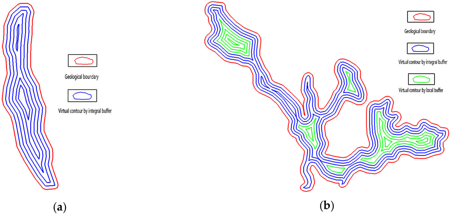
Planar virtual thickness contours of quaternary. (a) Planar virtual thickness contours of quaternary constructed by integral buffer and (b) planar virtual thickness contours of quaternary constructed by integral buffer and local buffer.

Figure 4 shows the flow chart of building the quaternary bottom interfaces and design sketches. In Figure 4a, the closed geological boundaries of quaternary were set as 0 m thickness contours. The appropriate buffer distance R was set according to the spatial coordinate range of each geological boundary. According to the set buffer distance R, we buffered the quaternary geological boundaries to the interior and recorded the maximum buffer times n (n is a positive integer). The average thickness H of quaternary recorded on the comprehensive stratigraphic column chart was divided by n, and the result was recorded as H/n. From the outside to the inside, the corresponding thickness values of planar virtual thickness contours were H/n, 2 H / n , … , H . Thus, a series of planar virtual thickness contours with a thickness difference of H/n were obtained (Figure 4b).

Figure 4

The flow chart of building quaternary bottom interfaces and design sketches. (a) Quaternary geological boundaries; (b) planar virtual thickness contours of quaternary; (c) virtual thickness contours of quaternary projected to topography; (d) 3D virtual thickness contours of quaternary; (e) triangular network of quaternary bottom interfaces; (f) quaternary bottom interfaces and topography.

Figure 4c shows the projection effect of the virtual thickness contours of quaternary on topography. The thickness value of the virtual thickness contours projected on topography was linearly transformed to the corresponding depth value H/n, 2 H / n , … , H . Thus, the 3D virtual thickness contours as shown in Figure 4d can be obtained.

As shown in Figure 4e, the Delaunay triangulation algorithm was used to process the 3D virtual thickness contours. In order to ensure that the quaternary bottom interfaces can cut the bedrock geological bodies, the quaternary bottom interfaces constructed must rise above the topography along the geological boundaries. Therefore, before triangulation of each group of 3D virtual thickness contours, it is necessary to copy the quaternary geological boundary and raise it by linear transformation for a certain distance. In Figure 4f, the triangular surface below the topography is the quaternary bottom interfaces.

2.2 Construction of bedrock interfaces

IDW is the most commonly used local spatial interpolation method in geological data processing. The basic idea of IDW spatial interpolation is that the closer the sample is to the point to be evaluated, the greater the weight obtained; otherwise, the smaller the weight obtained. In this paper, the geological map we discussed is characterized by large-scale and complex geological conditions. The occurrence data points are very sparse. Therefore, the IDW method is used to interpolate the occurrence data of the control points of bedrock geological boundaries. The attributes of occurrence data points include dip direction and dip angle.

Formula (1) is used to calculate the attributes of occurrence points to be estimated. Z*(x) represents the dip direction or dip angle value of the occurrence points to be estimated on the geological boundaries of bedrock. n is the number of actual occurrence points involved in the valuation. The specific value of n should be set according to the actual situation. Each control point on the geological boundaries is set to the center of the search sphere. The sphere is used to search for the n measured occurrence points nearest to the current control point of geological boundaries. Z(x _i) is the dip direction or dip angle attribute value of the measured occurrence point x _i searched in the sphere. λ _i is the weight assigned to x _i. Formula (2) is a classical formula for calculating λ _i; d _i is the distance between the measured occurrence point x _i and the estimated occurrence point x. The power exponent p of d _i can be any natural number or decimal; the larger the power p is, the greater the weight of occurrence points is; p is usually taken as 2.

(1) z ⁎ ( x ) = ∑ i = 1 n [ λ ⋅ z ( x i ) ]

(2) λ i = 1 d i p ∑ i = 1 n 1 d i p

Through the occurrence interpolation algorithm based on IDW, the control points on the geological boundaries obtain the occurrence attribute values of dip direction and dip angle. The occurrence data can be converted into occurrence tangent vector (X, Y, Z). Under the constraint of the occurrence tangent vectors, the bedrock geological boundaries extend to the underground to construct the bedrock geological interfaces. Figure 5 shows the flow chart of building bedrock geological interfaces based on IDW occurrence interpolation algorithm.

(3) X = cos(radians( β )) ⋅ sin(radians( α )) Y = cos(radians( β )) ⋅ cos (radians( α )) Z = − sin(radians( β ))

(4) X 2 = X 1 + D sin ( radians ( β ) ) ⋅ X = X 1 + ∣ H − Z 1 ∣ cot ( radians ( β ) ) ⋅ sin ( radians ( α ) ) Y 2 = Y 1 + D sin ( radians ( β ) ) ⋅ Y = Y 1 + ∣ H − Z 1 ∣ cot ( radians ( β ) ) ⋅ cos ( radians ( α ) ) Z 2 = H

Figure 5

The flow chart of building bedrock geological interfaces based on IDW.

It is assumed that the occurrence data are expressed as “α < β” (0° ≤ α < 360° and 0° < β ≤ 90°), α is dip direction, and β is dip angle. In Figure 6a, N points to the north, L1 represents the geological boundary, M1 (X1, Y1, Z1) is the control point on L1, and α and β represent the dip direction and dip angle of M1, respectively. M2 (X2, Y2, Z2) is the intersection point between the occurrence tangent direction of M1 and the bottom interface of the model. Suppose that the elevation of the bottom interface of the model is H, the elevation of M2 is H too. The vertical distance D of M1 and M2 is | H − Z1|. According to the formula (3), the occurrence of M1 (α < β) is converted into tangent vector (X, Y, Z). The occurrence tangent vector of M1 is brought into formula (4) to calculate the spatial coordinate of M2. Figure 6b shows the bedrock interfaces constructed under the constraint of occurrence tangent vectors.

Figure 6

(a) The sketch map of occurrence tangent vector and (b) the bedrock interfaces constructed under the constraint of occurrence tangent vectors.

The flow chart of building bedrock interfaces based on IDW and design sketches is shown Figure 7. The geological boundaries and the distribution of occurrence points are shown in Figure 7a. First, the geological boundaries and actual occurrence points need to be projected on topography (Figure 7b). Second, we apply the IDW occurrence interpolation algorithm to estimate the occurrence of the control points on geological boundaries (Figure 7c). Lastly, we construct the bedrock interfaces under the constraint of occurrence tangent vectors (Figure 7d).

Figure 7

The flow chart of building bedrock geological interfaces based on IDW and design sketches. (a) Bedrock geological boundaries and actual occurrence points; (b) bedrock geological boundaries and actual occurrence points projected on topographic surface; (c) discrete control points on bedrock geological boundaries; (d) bedrock geological interfaces.

2.3 Construction of fault interfaces

The construction method of fault interfaces is similar to that of bedrock interfaces. The extension trends of fault interfaces in underground are controlled by the tangent vectors of fault occurrence points. Figure 8 shows the construction example of fault interfaces. There is only one actual measured occurrence point near Fault A. The extension trend of Fault A is controlled by the same occurrence tangent vector value. There are two actual measured occurrence points near Fault B. The IDW interpolation algorithm can be used to interpolate the occurrence data of the control points on Fault line B. The extension trend of Fault B is controlled by multiple different occurrence tangent vector values.

Figure 8

Construction example of fault interfaces.

The intersection of faults in underground space is complex. We will use Binary Space Partitioning vector cutting algorithm to deal with the topological relationship between faults. Figure 9 presents the treatment of topological relationship between Fault C and Fault D. There is only one actual occurrence point near Fault C and three actual occurrence points near Fault D. The actual occurrence data of Fault C and Fault D are listed in Table 1. The IDW occurrence interpolation algorithm is used to estimate the occurrence data of control points on fault D. Table 2 presents the occurrence data of control points on Fault D.

Figure 9

The treatment of topological relationship between faults. (a) Fault C and fault d before treatment; (b) Fault C and fault d after treatment.

Table 1

The actual measured occurrence data of Fault C and Fault D

Fault name	Occurrence points	Dip direction	Dip angle
Fault C	M	30	38
Fault D	M1	145	36
	M2	150	25
	M3	155	30

Table 2

The estimated occurrence data of control points on Fault D

Fault name	Control points	Dip direction	Dip angle
Fault D	B-p1	153.594	29.565
	B-p2	153.747	29.593
	B-p3	154.023	29.654
	B-p4	154.315	29.735
	B-p5	154.49	29.791
	B-p6	154.747	29.886
	B-p7	154.863	29.931
	B-p8	154.788	29.886
	B-p9	154.256	29.553
	B-p10	153.113	28.724
	B-p11	151.683	27.474
	B-p12	150.602	26.254
	B-p13	150.121	25.462
	B-p14	150.021	25.234
	B-p15	149.934	25.608
	B-p16	149.489	27.02
	B-p17	148.424	29.517
	B-p18	146.951	32.49
	B-p19	146.135	34.013
	B-p20	145.297	35.5
	B-p21	145.027	35.957
	B-p22	145.055	35.912
	B-p23	145.272	35.576
	B-p24	145.346	35.463

2.4 Construction of 3D geological bodies

The construction sequences of 3D geological bodies are the construction of initial geological body, quaternary geological bodies, and bedrock geological bodies. Figure 10 shows the flow chart of constructing 3D geological bodies and design sketches. First, the top surface of the model is topography, and the bottom surface of the model is set to a uniform elevation depth. As shown in Figure 10a, the top and bottom surfaces are closed to construct the initial 3D geological body. Second, the vector cutting algorithm based on Binary Space Partitioning tree is used to deal with the shear operation between the quaternary bottom interfaces and the initial geological body (Figure 10b). As shown in Figures 10c and d, the quaternary geological bodies are extracted. Finally, the vector cutting algorithm based on Binary Space Partitioning tree is used to deal with the shear operation between bedrock interfaces and residual initial geological body (Figure 10e). The 3D geological modeling units of bedrock are constructed (Figure 10f).

Figure 10

The flow chart of constructing 3D geological bodies and design sketches. (a) Initial geological body; (b) quaternary bottom interfaces and initial geological body; (c) quaternary geological bodies and residual geological body; (d) separate quaternary geological bodies and residual geological body; (e) bedrock geological interfaces and residual geological body; (f) bedrock geological bodies.

3 Data organization of geological maps

According to the working standard of China Geological Survey [27], a complete geological map usually includes the main body (planar geological map), geological section map, comprehensive stratigraphic column chart, title, scale, legend, and other auxiliary elements. Figure 11 is the conceptual model of a geological map. The data in planar geological map can be divided into basic geographic data and geological data. The former mainly includes water system, traffic, residential area, boundaries, and topography, while the latter mainly includes strata, volcanic rocks, informal stratigraphic units, intrusive rocks, and other auxiliary elements. The geological section map can reflect the geological structure of deep strata. The comprehensive stratigraphic column chart is a map compiled according to the stratigraphic age sequence, contact relationship, and thickness in a region.

Figure 11

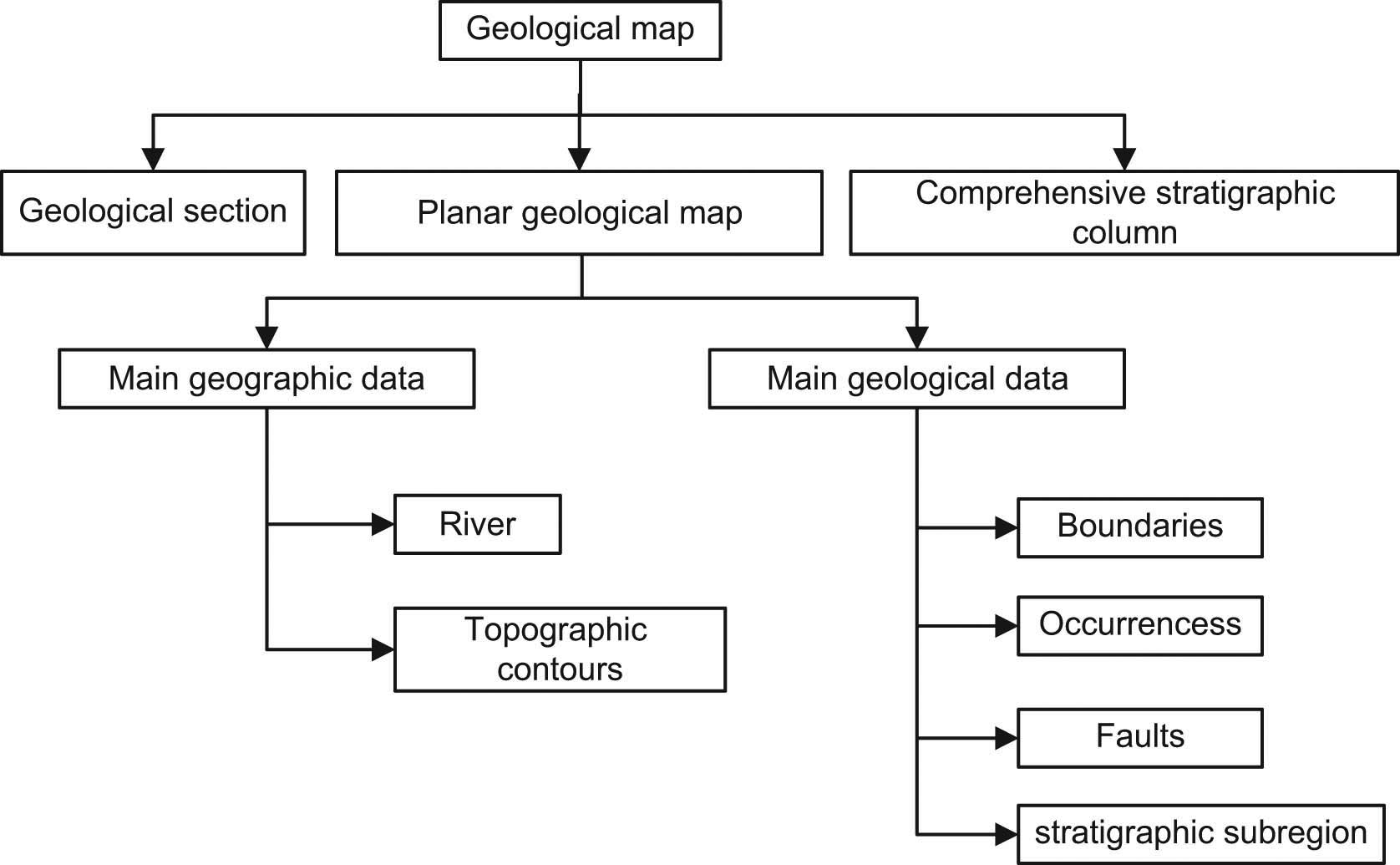
Conceptual model of geological maps.

According to different element types, the information in a geological map can be organized by point, line, and surface data. The point data are mainly occurrence marking points, which are generally located near the stratigraphic boundaries and fault lines. The line data mainly include stratigraphic boundaries, fault lines, topographic contours, and map border line. The surface data are mainly the stratigraphic surfaces, which contain the stratigraphic age, lithology, and other information.

4 A real application

In this paper, we have integrated two algorithms into a new workflow to construct 3D geological framework models of shallow strata by using large-scale geological maps. This modeling workflow has been implemented on QuanytView3D. Quantyview3D is a 3D visualization development platform for Geosciences. In order to verify the effectiveness of this modeling workflow, we built a 3D geological framework model of underground 300 m based on a geological map of a city in southern China.

4.1 Data

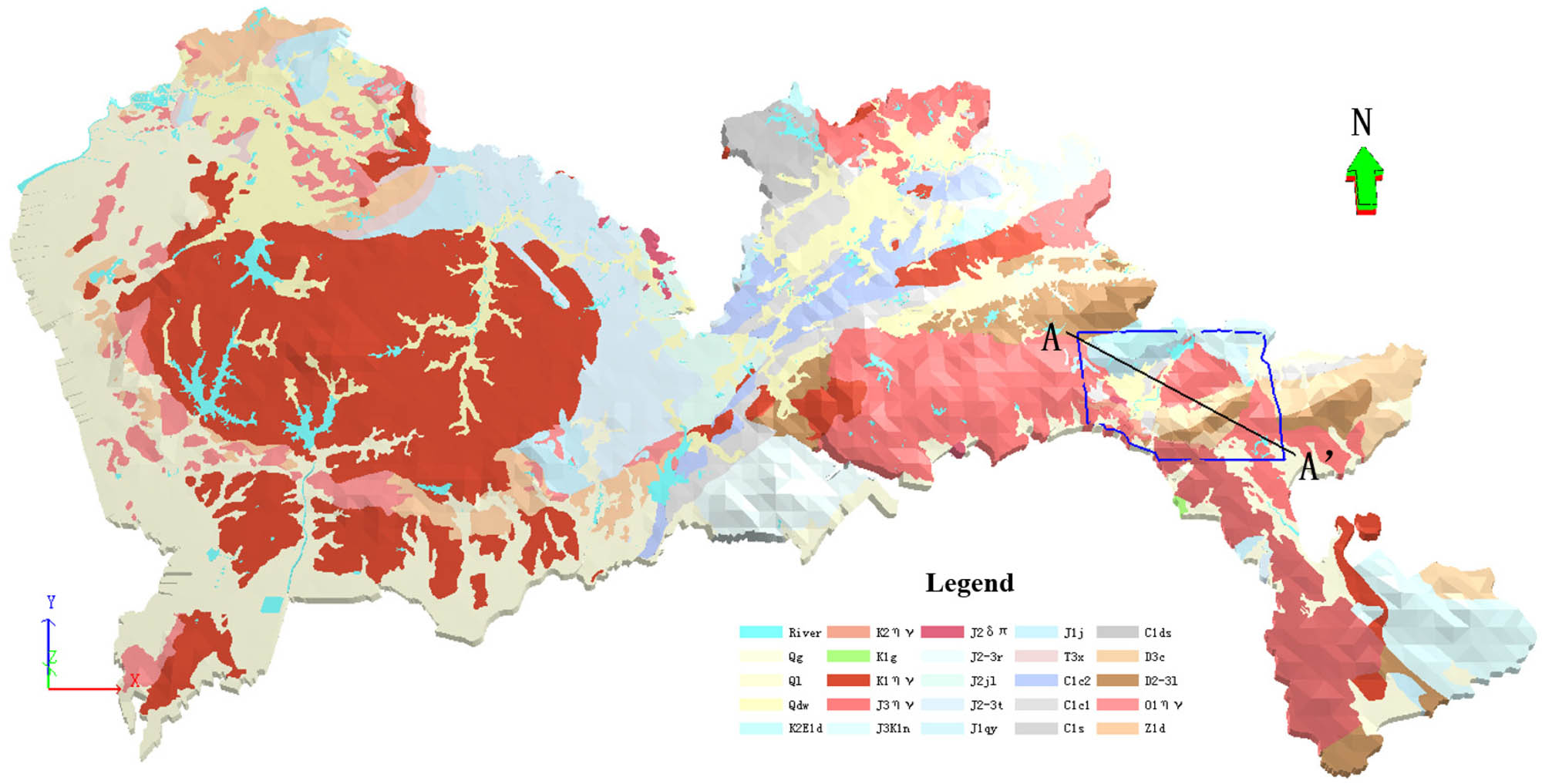
The geological map of a city in southern China is shown in Figure 12. The area of the whole city is 1,991 km². The lithology-stratigraphy mainly includes quaternary, igneous, and carbonate rocks. The average thickness of quaternary overburden is 0.5–28.6 m. The types and quantities of points, lines, and surfaces data in the planar geological map of the city are listed in Table 3.The data characteristics of the urban geological map are summarized as follows: (1) the spatial scale is large and the measured strata occurrence points are sparse; (2) the quaternary overburden with complex spatial morphology is widely distributed. In this paper, the quaternary is defined as overburden, other strata are defined as bedrock.

Figure 12

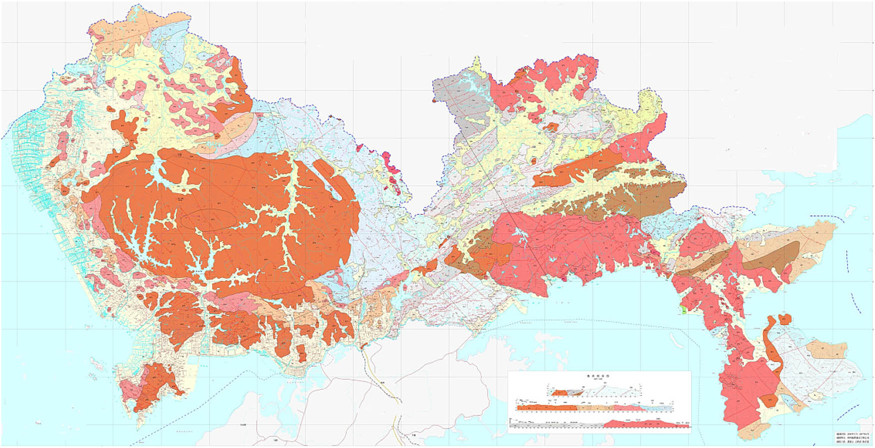
The geological map of a city in southern China.

Table 3

Data organization of the geological map of a city in southern China

Data set	Data item	Data type	Number
Geographic data set	River system	Line and surface
Geographic data set	Topographic contour	Line	12,753
Geological data set	Stratigraphic boundary	Line	662
	Fault line	Line	300
	Strata occurrence point	Point	234
	Fault occurrence point	Point	300
	Stratigraphic subregion	Surface	984

Figure 13 depicts the data processing results of the geological map of a city in southern China. The data were transferred to QuantyView3D through 2D to 3D spatial mapping relationship. The original attribute values were added for each element by using the information marked on the geological map.

Figure 13

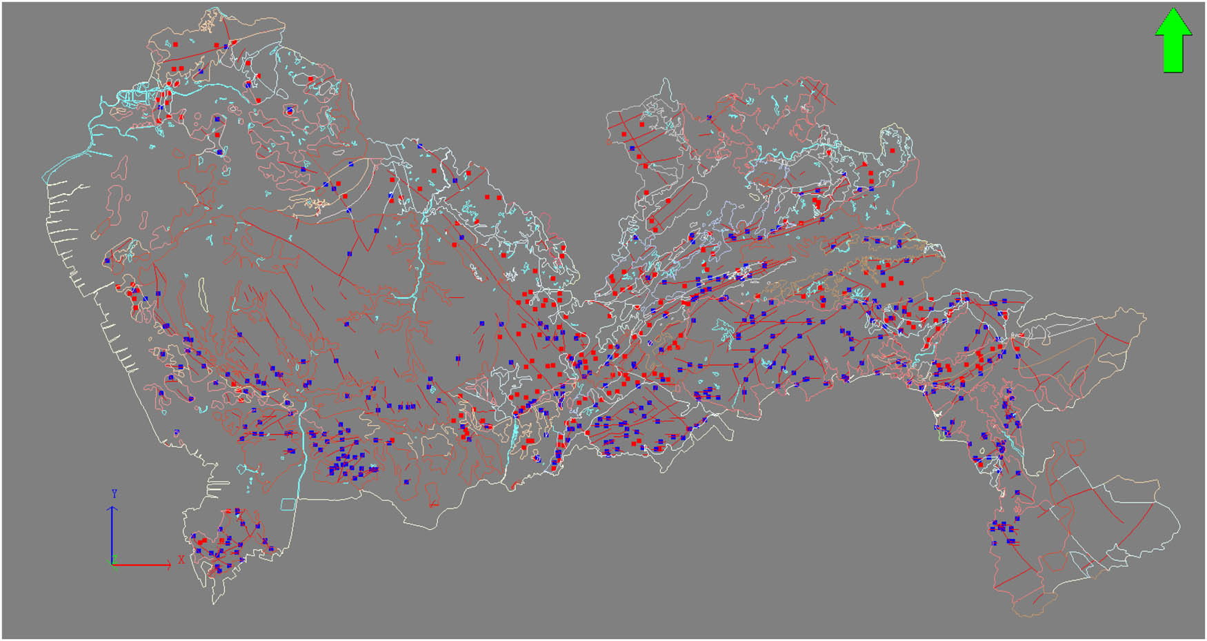
The data processing results of the geological map of a city in southern China.

4.2 Results and analysis

Because the depth of geological interfaces extending underground under the control of occurrence is limited, it is necessary to set a reasonable elevation depth for the bottom surface of the model. According to the geological background of the city and knowledge of geological experts, it is reasonable to set the elevation of the bottom of the model as −300 m. Figure 14 presents the 3D geological framework model of 300 m underground of a city in southern China. The model includes 69 quaternary geological bodies, 162 igneous geological bodies, 155 carbonate geological bodies, 83 other types of geological bodies, and 300 fault surfaces.

Figure 14

3D geological framework model of 300 m underground of a city in southern China.

The model of the whole city is relatively large; we extract the local model in the blue border from the whole model for analysis and verification. The fault network of local model is shown in Figure 15. The extension trends of the faults in the underground space are strictly restricted by the occurrences of the faults. The intersection relationships between the faults are also well-handled. We can cut the 3D geological model from any direction and get geological sections in any direction. The locations of 8 × 8 cross slices and AA’ slice are shown in Figure 16. And Figure 17 presents the 8 × 8 cross geological sections and AA’ geological section. From the geological sections, we can more intuitively understand the development form and spatial contact relationship of underground geological bodies. We select AA’ section to illustrate the effectiveness of the modeling results. Figure 18 shows the AA’ geological section of the local geological model. Figure 19 is the AA’ map-cut-section of the local geological map made by geological expert. The range and thickness of quaternary strata in Figure 18 are basically the same as those in Figure 19. The virtual thickness contour constructed by buffer algorithm can well-simulate the complex morphologies of the quaternary. The contact relationship between the quaternary overburden and the bedrock is also described in detail. The underground extension of bedrock geological interfaces in Figure 18 is similar to that in Figure 19. Through IDW occurrence interpolation, the geological interfaces of bedrock are reasonably constrained. In a word, the modeling results are consistent with the urban geological map interpreted by experts, which verifies the effectiveness of our modeling workflow. So we can build underground tunnels along the planned lines to provide auxiliary basis for urban planning. An example of tunnel excavation of the local model area is shown in Figure 20.

Figure 15

The fault network of zone B.

Figure 16

The 8 × 8 cross slices and AA’ slice of local model.

Figure 17

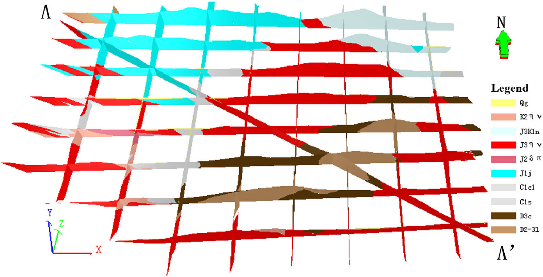
The 8 × 8 cross geological sections and AA’ geological section of local model.

Figure 18

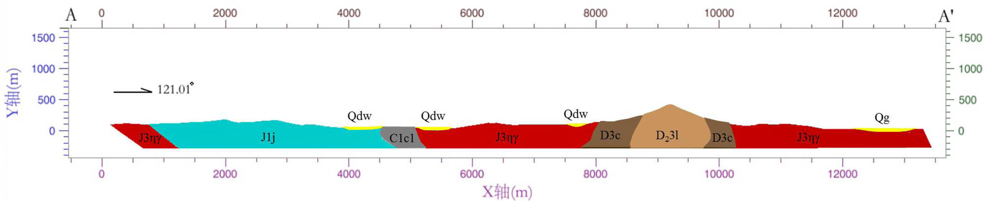
AA’ geological section of the local model.

Figure 19

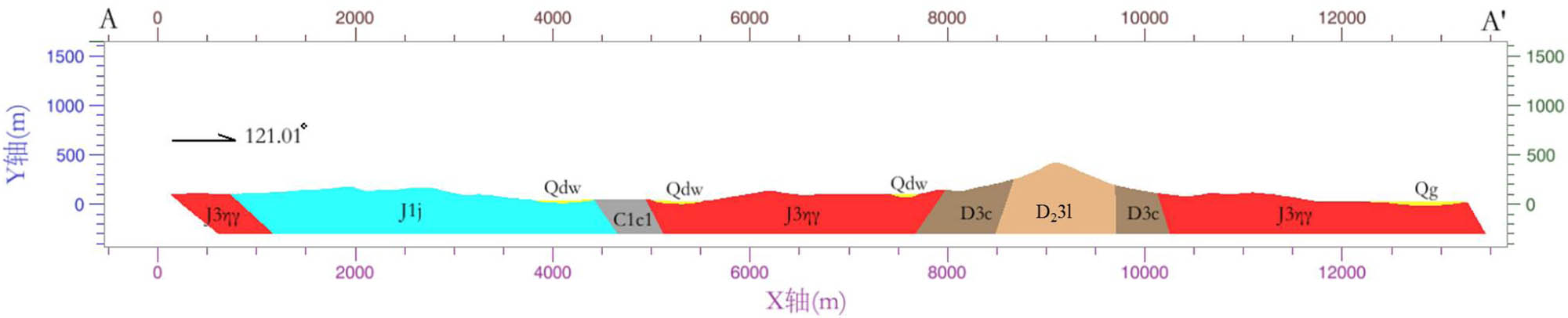
AA’ map-cut-section of the local geological map.

Figure 20

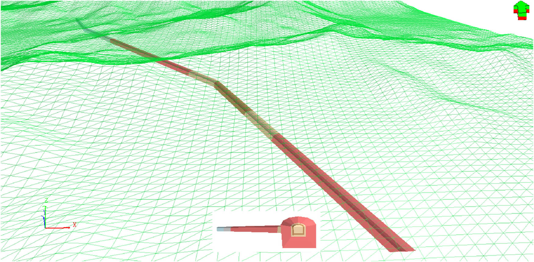
An example of tunnel excavation of the local model.

5 Conclusion

For the large-scale geological maps, we propose a new modeling workflow of constructing 3D geological framework models of shallow strata. We have integrated and implemented the modeling workflow on QuantyView3D. Taking a city in southern China as the data source, we have constructed a 3D geological framework model of underground 300 m by this workflow successfully. Through the virtual thickness contours constructed by the internal buffer algorithm of closed lines, we have effectively simulated the complex bottom interfaces of quaternary overburden. The complex contact relationships between quaternary overburden and bedrock were described in detail. The occurrence interpolation algorithm based on IDW has been used to constrain the extended trends of bedrock geological interfaces in the underground reasonably. The topological relations between different geological objects have been treated effectively by using the Binary Space Partitioning vector cutting algorithm. The 3D geological framework models of urban shallow strata constructed by our workflow accord with the semantic relationship of tectonics. The effectiveness of our modeling workflow has been verified. Through the 3D geological framework model, we can get the 3D geological sections in any direction. From the 3D geological sections, we can more intuitively understand the complex spatial structure of shallow strata. Through the analysis of underground tunnel excavation, it can provide auxiliary basis for urban planning. The construction of this 3D geological framework model also lays a foundation for the fine modeling after adding boreholes and sections. Therefore, we will study multisource data fusion technology and local dynamic updating technology of models in the next work, so as to build a more refined 3D geological model of urban shallow strata quickly.

Acknowledgements

This research was funded by Natural Science Foundation of China (U1711267, 41942039), Hubei Province Innovation Group Project (2019CFA023), the Fundamental Research Funds for the Central Universities (CUGL180823, CUG2019ZR03, CUGCJ1810). State Key Laboratory of Biogeology and Environmental Geology, China University of Geoscience.

Author contributions: Conceptualization: Gang Liu and Zhengping Weng; methodology: Xuechao Wu, Zhengping Weng, Yiping Tian, and Zhiting Zhang; software: Xuechao Wu; validation: Gang Liu and Zhengping Weng; formal analysis: Xuechao Wu; data curation: Yang Li and Xuechao Wu; writing-original draft preparation: Xuechao Wu; visualization: Xuechao Wu and Genshen Chen; supervision: Gang Liu. All authors have read and agreed to the published version of the manuscript.
Conflicts of interest: The authors declare no conflict of interest.

References

[1] Houlding SW. 3D geoscience modeling-computer techniques for geological characterization. New York & Heidelburg: Springer-Verlag; 1994. p. 1–30910.1007/978-3-642-79012-6Suche in Google Scholar

[2] Chen QY, Liu G, Li XC, Zhang ZT, Li Y. A corner-point-grid-based voxelization method for the complex geological structure model with folds. J Vis. 2017;20(4):875–88.10.1007/s12650-017-0433-7Suche in Google Scholar

[3] He HH, He J, Xiao JZ, Zhou YX, Liu Y, Li C. 3D geological modeling and engineering properties of shallow superficial deposits: a case study in Beijing, China. Tunn Undergr Sp Tech. 2020;100:103390.10.1016/j.tust.2020.103390Suche in Google Scholar

[4] Zhang XY, Zhang JQ, Tian YP, Li ZL, Zhang Y, Xu LR, et al. Urban geological 3D modeling based on papery Borehole log. ISPRS Int J Geo-Inf. 2020;9(6):389.10.3390/ijgi9060389Suche in Google Scholar

[5] Chen QY, Liu G, Mao XG, Yao Z, Tian YP, Wang HL. A virtual globe-based integration and visualization framework for aboveground and underground 3D spatial objects. Earth Sci Inf. 2018;11(4):591–603.10.1007/s12145-018-0350-xSuche in Google Scholar

[6] Miquel V, Pau T, Roser P, David A, Ona M. The role of 3D modeling in the urban geological map of Catalonia. Z Dtsch Ges Geowiss. 2016;167(4):389–403.10.1127/zdgg/2016/0095Suche in Google Scholar

[7] Xiong ZM, Guo JT, Xia YP, Lu H, Wang MY, Shi SS. A 3D multi-scale geology modeling method for tunnel engineering risk assessment. Tunn Undergr Sp Tech. 2018;73:71–81.10.1016/j.tust.2017.12.003Suche in Google Scholar

[8] Jiskani IM, Siddiqui FI, Pathan AG. Integrated 3D geological modeling of Sonda-Jherruck coal field, Pakistan. J Sustain Min. 2018;17(3):111–9.10.1016/j.jsm.2018.06.001Suche in Google Scholar

[9] Zhu LF, Zhang CJ, Li MJ, Pan X, Sun JZ. Building 3D solid models of sedimentary stratigraphic systems from borehole data: an automatic method and case studies. Eng Geol. 2012;127:1–13.10.1016/j.enggeo.2011.12.001Suche in Google Scholar

[10] Chen QY, Mariethoz G, Liu G, Comunian A, Ma XG. Locality-based 3-D multiple-point statistics reconstruction using 2-D geological cross sections. Hydrol Earth Syst Sci. 2018;22(12):6547–66.10.5194/hess-22-6547-2018Suche in Google Scholar

[11] Wang GW, Zhu YY, Zhang ST, Yan CH. 3D geological modeling based on gravitational and magnetic data inversion in the Luanchuan ore region, Henan Province, China. J Appl Geophys. 2012;80(5):1–11.10.1016/j.jappgeo.2012.01.006Suche in Google Scholar

[12] Kaufmann O, Martin T. 3D geological modeling from boreholes, cross-sections and geological maps, application over former natural gas storages in coal mines. Comput Geosci-UK. 2008;34:278–90.10.1016/j.cageo.2007.09.005Suche in Google Scholar

[13] Qiao JH, Pan M, Li ZL, Yi J. 3D Geological modeling from DEM, boreholes, cross-sections and geological maps. 2011 19th International Conference on Geoinformatics, Shanghai, China: IEEE; 2011. p. 1–5.10.1109/GeoInformatics.2011.5980941Suche in Google Scholar

[14] Wu ZC, Guo FS, Li JT. The 3D modelling techniques of digital geological mapping. Arab J Geosci. 2019;12:467.10.1007/s12517-019-4615-6Suche in Google Scholar

[15] Benoît D, Hassan T, Fatima EL, Abdel-Ali C, Ahlam M, Meriam L, et al. Engineering geology for society and territory. Cham, Switzerland: Springer. Vol. 6; 2015. p. 101–5.10.1007/978-3-319-09060-3_18Suche in Google Scholar

[16] Zanchi A, Francesca S, Stefano Z, Simone S, Graziano G. 3D reconstruction of complex geological bodies: examples from the Alps. Comput Geosci-Uk. 2009;35(1):49–69.10.1016/j.cageo.2007.09.003Suche in Google Scholar

[17] Jiskani IM, Siddiqui FI. Fault orientation modeling of Sonda-Jherruck coalfield, Pakistan. JME. 2019;10(2):305–13.Suche in Google Scholar

[18] Amorim R, Brazil E, Samavati F, Sousa M. 3D geological modeling using sketches and annotations from geologic maps. Proceedings of the 4th Joint Symposium on Computational Aesthetics, Non-Photorealistic Animation and Rendering, and Sketch-Based Interfaces and Modeling. Aire-la-Ville, Switzerland: Eurographics Association; 2014. p. 17–2510.1145/2630407.2630411Suche in Google Scholar

[19] Guo JT, Wu LX, Zhou WH, Jiang JZ, Li CL. Towards automatic and topologically consistent 3D regional geological modeling from boundaries and attitudes. ISPRS Int J Geo-Inf. 2016;5(2):17.10.3390/ijgi5020017Suche in Google Scholar

[20] Macêdo I, Gois JP, Velho L. Hermite radial basis functions implicits. Computer graphics forum. Oxford, UK: Blackwell Publishing; 2011.10.1111/j.1467-8659.2010.01785.xSuche in Google Scholar

[21] Guo JT, Wu LX, Zhou WH, Jiang JZ, Li CL, Li FD. Section-constrained local geological interface dynamic updating method based on the HRBF surface. J Struct Geol. 2018;107:64–72.10.1016/j.jsg.2017.11.017Suche in Google Scholar

[22] Wang JM, Hui Z, Lin BX, Wang LG. Implicit 3D modeling of ore body from geological boreholes data using hermite radial basis functions. Minerals. 2018;8(10):443.10.3390/min8100443Suche in Google Scholar

[23] Zhou LC, Lin BX, Wang D, Lv GL. 3D geological modeling method based on planar geological map. J Geo-Inf Sci. 2013;15:46–54.10.3724/SP.J.1047.2013.00046Suche in Google Scholar

[24] Lin BX, Zhou LC, Lv GN, Zhu AX. 3Dgeological modelling based on 2D geological map. Ann GIS. 2017;23(2):117–29.10.1080/19475683.2017.1304450Suche in Google Scholar

[25] Zhang BY, Li Y, Chen XY, Hao D, Mao XC. Regional metallogenic geo-bodies 3D modeling and mineral resource assessment based on geologic map cut cross-sections: a case study of manganese deposits in southwestern Guangxi, China. J Jilin Univ (Earth Sci Ed). 2017;47:933–48.Suche in Google Scholar

[26] Chen QY, Liu G, Ma XG, Li XC, He ZW. 3D stochastic modeling framework for Quaternary sediments using multiple-point statistics: a case study in Minjiang Estuary area. Southeast China Comput Geosci-UK. 2020;136:104404.10.1016/j.cageo.2019.104404Suche in Google Scholar

[27] China Geological Survey. DD 2019-01 Technical requirement for regional geological survey (1:50,000), Beijing; 2019.Suche in Google Scholar

Received: 2020-11-16

Revised: 2021-06-04

Accepted: 2021-06-21

Published Online: 2021-08-09

This work is licensed under the Creative Commons Attribution 4.0 International License.

Artikel in diesem Heft

https://doi.org/10.1515/geo-2020-0270

Schlagwörter für diesen Artikel

3D geological modeling; large-scale geological maps; geological interfaces; virtual thickness contours; occurrence interpolation

Creative Commons

BY 4.0