Semi-analytical approximation of time-fractional telegraph equation via natural transform in Caputo derivative
-
Mamta Kapoor
 and
Samanyu Khosla
and
Samanyu Khosla

Abstract
In the present research study, time-fractional hyperbolic telegraph equations are solved iteratively using natural transform in one, two, and three dimensions. The fractional derivative is considered in the Caputo sense. These equations serve as a model for the wave theory process of signal processing and transmission of electric impulses. To evaluate the validity and effectiveness of the suggested strategy, a graphical comparison of approximated and exact findings is performed. Convergence analysis of the approximations utilising
Graphical abstract

1 Introduction
Fractional calculus is a branch of mathematics that deals with partial order integrals, derivatives, and their equations. It was initially alluded to in a letter written by L’ Hospital to Leibnitz, essentially asking about a derivative with order ½ [1]. As fractional calculus is further developed, it found its application in many domains, which includes variational calculus [2], random walks [3], optimal control theory [4], image processing [5], etc.
Second-order hyperbolic partial differential equations (PDE) known as telegraph equation, developed by Oliver Heaviside [6], is used to elaborate voltage and current in an electric transmission line. Further generalizing such equations, we come across a particular kind of equation, known as the fractional hyperbolic telegraph equation (FHTE). Being a type of fractional PDE (FPDE), it is quite a challenge to solve such an equation without using advanced numerical and analytical techniques. FPDEs have multiple methods developed by many researchers due to their importance, e.g., Kudryashov method, Bäcklund transformation method based on the Riccati equation, and a new auxiliary ordinary differential equation have been used to obtain obtaining optical soliton solutions for the Lakshmanan–Porsezian–Daniel model with Kerr law nonlinearity [7]. Laplace transform method has been used to solve constructive equations of the fractional second grade fluid [8]. An extension of homotopy analysis method using Laplace transform, called q-homotopy analysis transform method, was used to solve time and space fractional coupled Burgers’ equations [9]. The fractional reduced differential transform method has been used to obtain approximate solutions of time fractional gas dynamics equation [10]. A hybrid method of decomposition method and Elzaki transformation has been used to solve Navier–Stokes equation [11]. Fractional order diffusion equations were solved using natural transform decomposition [12]. Shallow water forced Korteweg–DeVries equation describing free surface critical flow over a hole has been solved using q-homotopy analysis transformed technique [13]. Variable-order time-space fractional KdV–Burgers–Kuramoto equation has been solved using a pseudo-operational collocation scheme [14]. A Vieta-Fibonacci collocation method has been used to solve fractional delay integro-differential equations [15]. A method based on Laplace transform and homotopy analysis method has been used to obtain approximate solutions of time fractional nonlinear water wave equation [16]. The homotopy analysis transform method using Laplace transform has been used to obtain the approximate solution of nonlinear time-fractional Cauchy reaction–diffusion equation [17].
Multiple techniques have been used to solve FHTEs. Khan et al. [18] used a new technique of adomian decomposition method (ADM) to solve fractional order hyperbolic telegraph equations. Sweilam et al. [19] approached time-fractional telegraph equations using the Sinc-Legendre collocation method. Saadatmandi and Mohabbati [20] employed a computational tau technique based on Legendre polynomials to solve time-fractional telegraph equations. A hybrid technique using Sumudu and Fourier transforms has been used to solve time fractional telegraph equation [21]. Shehu transform has been used to obtain series solution of FHTE [22]. For solving linear time-fractional telegraph equations, two-variable Vieta-Fibonacci polynomials have been constructed and coupled with a matrix collocation scheme [23].
1.1 One-dimensional fractional telegraph equation [ 22 ]
Here,
1.2 Two-dimensional fractional telegraph equation [ 22 ]
where
1.3 Three-dimensional fractional telegraph equation [22]
where
There exist different approaches to tackle FHTEs, and one such way is to apply an integral transform on the equation and obtain an iterative solution. Several integral transforms exist, such as Sumudu transform [24], natural transform [25], Shehu transform [26], and Elzaki transform [27]. These transforms can be applied on various techniques, such as homotopy perturbation method [28], ADM [29], reduced differential transform method [30], and generalized differential transform method [31] to obtain solutions to FHTEs. For example, Laplace Transform has been used for solving telegraph equations by implementing q-Homotopy Analysis Transform Method [32]. Natural transform was developed by Khan and Khan [25] in 2008 and was used to solve a certain kind of the fluid flow problem. Since then, it has found its application in many different cases, one such case being natural transform decomposition method (NTDM). NTDM has been used to solve fractional order partial differential equations [33] and Burgers’ equations [34]. In the present article, natural transform would be used to obtain an iterative semi analytical solution to FHTEs. Fractional order has been considered because of it being a more generalized form of hyperbolic telegraph equations, which means the integer order solutions can also be obtained using the appropriate value of fractional order. The approach is based on the one used in solving FHTEs using Shehu transform [22]. When developing the general formula, natural transform is applied on the equation. Linear and nonlinear operators are separated into sum of terms inverse natural transform is applied, which is then used to develop an iterative scheme (Tables 1 and 2).
Natural transform of common functions [36]
|
|
|
|
|---|---|---|
| 1 |
|
|
| 2 |
|
|
| 3 |
|
|
| 4 |
|
|
| 5 |
|
|
| 6 |
|
|
| 7 |
|
|
Inverse natural transform of common functions [36]
|
|
|
|
|---|---|---|
| 1 |
|
|
| 2 |
|
|
| 3 |
|
|
| 4 |
|
|
| 5 |
|
|
| 6 |
|
|
| 7 |
|
|
1.4 Basics of natural transform
Definition 1
Natural transform of a function [35].
where
Definition 2
Natural transform of fractional derivative in Caputo sense [35].
Theorem 1
Linearity property of natural transform [25].
where
Theorem 2
Change of scale property of natural transform [36].
where
Definition 3
Fractional derivative of a function in Caputo sense [37].
where
2 Development of the formula
2.1 Implementation upon 1D time-fractional telegraph equation
The form of 1D time-fractional telegraph equation is as follows [22]:
where
Now,
Therefore,
2.2 Implementation upon 2D time-fractional telegraph equation
The form of 2D time-fractional telegraph equation is as follows [22]:
See Appendix A.
2.3 Implementation upon 3D time-fractional telegraph equation
The form of 3D time-fractional telegraph equation is as follows [22]:
See Appendix B.
3 Examples and calculation
Example 1. Considered following 1D time-fractional telegraph equation [22]:
where
By applying natural transform on Eq. (1), we obtain:
By using Eq. (3), we obtain:
By using Eq. (3), we obtain:
By using Eq. (3), we obtain:
By using Eq. (3), we obtain:
By using Eq. (3), we obtain:
By considering
Example 2. Consider the following 1D time-fractional telegraph equation [22]:
where
By applying natural transform on Eq. (4), we obtain:
By using Eq. (6):
By using Eq. (6):
By using Eq. (6), we obtain:
By using Eq. (6), we obtain:
By using Eq. (6), we obtain:
By substituting
Example 3. Considered following nonlinear 1D time-fractional telegraph equation [22]:
where
By applying natural transform on Eq. (7), we obtain:
Consider Eq. (8):
By using Eq. (9), we obtain:
By using Eq. (10), we obtain:
By using Eq. (10), we obtain:
By using Eq. (10), we obtain:
By using Eq. (10), we obtain:
By using Eq. (10), we obtain:
By substituting
Example 4. Considered following nonlinear 1D time-fractional telegraph equation [22]:
where
Applying natural transform on Eq. (11):
By using Eq. (13), we obtain:
By using Eq. (13), we obtain:
By using Eq. (13), we obtain:
By using Eq. (13), we obtain:
By using Eq. (13), we obtain:
By substituting
Example 5. Considered following nonlinear 2D time-fractional telegraph equation [22]:
where
By applying natural transform on Eq. (14):
By using Eq. (16), we obtain:
By using Eq. (16), we obtain:
By using Eq. (16), we obtain:
By using Eq. (16), we obtain:
By using Eq. (16), we obtain:
By substituting
Example 6. Considered following nonlinear 3D time-fractional telegraph equation [22]:
where
By applying natural transform on Eq. (17), we obtain:
By using Eq. (19), we obtain:
By using Eq. (19), we obtain:
By using Eq. (19), we obtain:
By using Eq. (19), we obtain:
By using Eq. (19), we obtain:
By substituting
4 Graphical and tabular discussion
Figure 1 compares approximate and exact findings for Example 1 at

Examining the differences between approximate and exact findings for Example 1 at

Comparison of approximate and exact findings for Example 2 at

Comparison of approximate and exact findings for Example 3 at

Comparison of approximate and exact findings for Example 4 at

Comparison of findings for Example 5 at
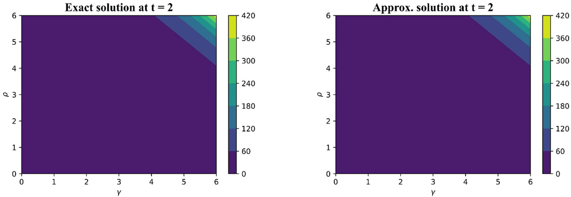
A comparison of roughly and precise outcomes for Example 5 at

Comparison of findings for Example 5 at
We define
Analysis of the errors in Examples 1 and 4
| N |
|
||
|---|---|---|---|
|
|
|
|
|
| 10 |
|
|
|
| 20 |
|
|
|
| 30 |
|
|
|
| ↓ | ↓ | ↓ | |
| Up to
|
Up to
|
Up to
|
|
Analysis of the errors in Example 2
|
|
|
||
|---|---|---|---|
|
|
|
|
|
| 10 |
|
|
|
| 20 |
|
|
|
| 30 |
|
|
|
| ↓ | ↓ | ↓ | |
| Up to
|
Up to
|
Up to
|
|
Analysis of the errors in Example 3
|
|
|
||
|---|---|---|---|
|
|
|
|
|
| 10 |
|
|
|
| 20 |
|
|
|
| 30 |
|
|
|
| ↓ | ↓ | ↓ | |
| Up to
|
Up to
|
Up to
|
|
Analysis of the errors in Example 5
|
|
|
||
|---|---|---|---|
|
|
|
|
|
| 10 |
|
|
|
| 15 |
|
|
|
| 20 |
|
|
|
| ↓ | ↓ | ↓ | |
| Up to
|
Up to
|
Up to
|
|
5 Conclusion
In the present article, the approximated and exact solutions of FHTEs in 1D, 2D, and 3D were obtained using an iterative approach using natural transform. Via graphical representation, it was observed that the approximate and exact graphs of Examples 1, 2 3, and 4 each taken at
-
Funding information: The authors state no funding involved.
-
Author contributions: All authors have accepted responsibility for the entire content of this manuscript and approved its submission.
-
Conflict of interest: The authors have no conflict of interest.
-
Data availability statement: All the data are included within the manuscript.
Appendix A
A.1 Implementation upon 2D time-fractional telegraph equation
The form of 2D time-fractional telegraph equation is as follows [22]:
where
Now,
Therefore,
Appendix B
A.2 Implementation upon 3D time-fractional telegraph equation
The form of 3D time-fractional telegraph equation is as follows [22]:
where
Now,
Therefore,
References
[1] Leibniz GW. Letter from Hanover, Germany to GFA L’Hospital, September 30, 1695. Math Schriften. 1849;2:301–2.Search in Google Scholar
[2] El‐Nabulsi RA, Torres DF. Necessary optimality conditions for fractional action‐like integrals of variational calculus with Riemann–Liouville derivatives of order (α, β). Math Methods Appl Sci. 2007;30(15):1931–9.10.1002/mma.879Search in Google Scholar
[3] Hilfer R, Anton L. Fractional master equations and fractal time random walks. Phys Rev E. 1995;51(2):R848.10.1103/PhysRevE.51.R848Search in Google Scholar
[4] Frederico GS, Torres DF. Fractional conservation laws in optimal control theory. Nonlinear Dyn. 2008;53:215–22.10.1007/s11071-007-9309-zSearch in Google Scholar
[5] Yi-Fei PU. Fractional differential analysis for texture of digital image. J Algorithms Comput Technol. 2007;1(3):357–80.10.1260/174830107782424075Search in Google Scholar
[6] Saad A, Brahim N. An efficient algorithm for solving the conformable time-space fractional telegraph equations. Moroccan J Pure Appl Anal. 2021;7(3):413–29.10.2478/mjpaa-2021-0028Search in Google Scholar
[7] Rezazadeh H, Kumar D, Neirameh A, Eslami M, Mirzazadeh M. Applications of three methods for obtaining optical soliton solutions for the Lakshmanan–Porsezian–Daniel model with Kerr law nonlinearity. Pramana. 2020;94:1.10.1007/s12043-019-1881-5Search in Google Scholar
[8] Sene N. Second-grade fluid with Newtonian heating under Caputo fractional derivative: analytical investigations via Laplace transforms. Math Model Numer Simul Appl. 2022;2(1):13–25.10.53391/mmnsa.2022.01.002Search in Google Scholar
[9] Singh J, Kumar D, Swroop R. Numerical solution of time-and space-fractional coupled Burgers’ equations via homotopy algorithm. Alex Eng J. 2016;55(2):1753–63.10.1016/j.aej.2016.03.028Search in Google Scholar
[10] Singh BK, Kumar P. Numerical computation for time-fractional gas dynamics equations by fractional reduced differential transforms method. J Math Syst Sci. 2016;6(6):248–59.10.17265/2159-5291/2016.06.004Search in Google Scholar
[11] Khan H, Khan A, Kumam P, Baleanu D, Arif M. An approximate analytical solution of the Navier–Stokes equations within Caputo operator and Elzaki transform decomposition method. Adv Differ Equ. 2020;2020:1–23.10.1186/s13662-020-02839-ySearch in Google Scholar
[12] Shah R, Khan H, Mustafa S, Kumam P, Arif M. Analytical solutions of fractional-order diffusion equations by natural transform decomposition method. Entropy. 2019;21(6):557.10.3390/e21060557Search in Google Scholar PubMed PubMed Central
[13] Veeresha P, Yavuz M, Baishya C. A computational approach for shallow water forced Korteweg–De Vries equation on critical flow over a hole with three fractional operators. An Int J Optim Control Theories Appl (IJOCTA). 2021;11(3):52–67.10.11121/ijocta.2021.1177Search in Google Scholar
[14] Sadri K, Hosseini K, Hinçal E, Baleanu D, Salahshour S. A pseudo‐operational collocation method for variable‐order time‐space fractional KdV–Burgers–Kuramoto equation. Math Methods Appl Sci. 2023.10.1002/mma.9015Search in Google Scholar
[15] Sadri K, Hosseini K, Baleanu D, Salahshour S, Park C. Designing a matrix collocation method for fractional delay integro-differential equations with weakly singular kernels based on Vieta–Fibonacci polynomials. Fractal Fract. 2022;6(1):2.10.3390/fractalfract6010002Search in Google Scholar
[16] Hosseini K, Ilie M, Mirzazadeh M, Yusuf A, Sulaiman TA, Baleanu D, et al. An effective computational method to deal with a time-fractional nonlinear water wave equation in the Caputo sense. Math Comput Simul. 2021;187:248–60.10.1016/j.matcom.2021.02.021Search in Google Scholar
[17] Hosseini K, Ilie M, Mirzazadeh M, Baleanu D. An analytic study on the approximate solution of a nonlinear time‐fractional Cauchy reaction–diffusion equation with the Mittag–Leffler law. Math Methods Appl Sci. 2021;44(8):6247–58.10.1002/mma.7059Search in Google Scholar
[18] Khan H, Khan Q, Kumam P, Tchier F, Singh G, Sitthithakerngkiet K, et al. A new modified technique to study the dynamics of fractional hyperbolic-telegraph equations. Open Phys. 2022;20(1):764–77.10.1515/phys-2022-0072Search in Google Scholar
[19] Sweilam NH, Nagy AM, El-Sayed AA. Solving time-fractional order telegraph equation via Sinc–Legendre collocation method. Mediterr J Math. 2016;13:5119–33.10.1007/s00009-016-0796-3Search in Google Scholar
[20] Saadatmandi A, Mohabbati M. Numerical solution of fractional telegraph equation via the tau method. Math Rep. 2015;17(67):2.Search in Google Scholar
[21] Dubey RS, Goswami P, Belgacem FB. Generalized time-fractional telegraph equation analytical solution by Sumudu and Fourier transforms. J Fract Calculus Appl. 2014;5(2):52–8.Search in Google Scholar
[22] Kapoor M, Shah NA, Saleem S, Weera W. An analytical approach for fractional hyperbolic telegraph equation using Shehu transform in one, two and three dimensions. Mathematics. 2022;10(12):1961.10.3390/math10121961Search in Google Scholar
[23] Sadri K, Hosseini K, Baleanu D, Salahshour S. A high-accuracy Vieta-Fibonacci collocation scheme to solve linear time-fractional telegraph equations. Waves Random Complex Media. 2022;1–24.10.1080/17455030.2022.2135789Search in Google Scholar
[24] Watugala G. Sumudu transform: a new integral transform to solve differential equations and control engineering problems. Integr Educ. 1993 Jan 1;24(1):35–43.10.1080/0020739930240105Search in Google Scholar
[25] Khan ZH, Khan WA. N-transform-properties and applications. NUST J Eng Sci. 2008;1(1):127–33.Search in Google Scholar
[26] Maitama S, Zhao W. New integral transform: Shehu transform a generalization of Sumudu and Laplace transform for solving differential equations. arXiv preprint. arXiv:1904.11370; 2019 Apr 19.Search in Google Scholar
[27] Elzaki TM. The new integral transform Elzaki transform. Glob J Pure Appl Math. 2011;7(1):57–64.Search in Google Scholar
[28] Yıldırım A. He’s homotopy perturbation method for solving the space-and time-fractional telegraph equations. Int J Comput Math. 2010;87(13):2998–3006.10.1080/00207160902874653Search in Google Scholar
[29] Garg M, Sharma A. Solution of space-time fractional telegraph equation by Adomian decomposition method. J Inequal Spec Funct. 2011;2(1):1–7.Search in Google Scholar
[30] Srivastava VK, Awasthi MK, Kumar S. Analytical approximations of two and three dimensional time-fractional telegraphic equation by reduced differential transform method. Egypt J Basic Appl Sci. 2014;1(1):60–6.10.1016/j.ejbas.2014.01.002Search in Google Scholar
[31] Garg M, Manohar P, Kalla SL. Generalized differential transform method to space-time fractional telegraph equation. Int J Differ Equ. 2011;2011:548982.10.1155/2011/548982Search in Google Scholar
[32] Prakash A, Veeresha P, Prakasha DG, Goyal M. A homotopy technique for a fractional order multi-dimensional telegraph equation via the Laplace transform. Eur Phys J Plus. 2019;134:1–8.10.1140/epjp/i2019-12411-ySearch in Google Scholar
[33] Eltayeb H, Abdalla YT, Bachar I, Khabir MH. Fractional telegraph equation and its solution by natural transform decomposition method. Symmetry. 2019;11(3):334.10.3390/sym11030334Search in Google Scholar
[34] Aljahdaly NH, Agarwal RP, Shah R, Botmart T. Analysis of the time fractional-order coupled burgers equations with non-singular kernel operators. Mathematics. 2021;9(18):2326.10.3390/math9182326Search in Google Scholar
[35] Zhou MX, Kanth AR, Aruna K, Raghavendar K, Rezazadeh H, Inc M, et al. Numerical solutions of time fractional Zakharov-Kuznetsov equation via natural transform decomposition method with nonsingular kernel derivatives. J Funct Spaces. 2021;2021:1–7.10.1155/2021/9884027Search in Google Scholar
[36] Belgacem FB, Silambarasan R. Theory of natural transform. Math Engg Sci Aeros. 2012;3:99–124.10.1063/1.4765477Search in Google Scholar
[37] Srivastava VK, Awasthi MK, Tamsir M. RDTM solution of Caputo time fractional-order hyperbolic telegraph equation. AIP Adv. 2013;3(3):032142.10.1063/1.4799548Search in Google Scholar
© 2023 the author(s), published by De Gruyter
This work is licensed under the Creative Commons Attribution 4.0 International License.
Articles in the same Issue
- Research Articles
- The regularization of spectral methods for hyperbolic Volterra integrodifferential equations with fractional power elliptic operator
- Analytical and numerical study for the generalized q-deformed sinh-Gordon equation
- Dynamics and attitude control of space-based synthetic aperture radar
- A new optimal multistep optimal homotopy asymptotic method to solve nonlinear system of two biological species
- Dynamical aspects of transient electro-osmotic flow of Burgers' fluid with zeta potential in cylindrical tube
- Self-optimization examination system based on improved particle swarm optimization
- Overlapping grid SQLM for third-grade modified nanofluid flow deformed by porous stretchable/shrinkable Riga plate
- Research on indoor localization algorithm based on time unsynchronization
- Performance evaluation and optimization of fixture adapter for oil drilling top drives
- Nonlinear adaptive sliding mode control with application to quadcopters
- Numerical simulation of Burgers’ equations via quartic HB-spline DQM
- Bond performance between recycled concrete and steel bar after high temperature
- Deformable Laplace transform and its applications
- A comparative study for the numerical approximation of 1D and 2D hyperbolic telegraph equations with UAT and UAH tension B-spline DQM
- Numerical approximations of CNLS equations via UAH tension B-spline DQM
- Nonlinear numerical simulation of bond performance between recycled concrete and corroded steel bars
- An iterative approach using Sawi transform for fractional telegraph equation in diversified dimensions
- Investigation of magnetized convection for second-grade nanofluids via Prabhakar differentiation
- Influence of the blade size on the dynamic characteristic damage identification of wind turbine blades
- Cilia and electroosmosis induced double diffusive transport of hybrid nanofluids through microchannel and entropy analysis
- Semi-analytical approximation of time-fractional telegraph equation via natural transform in Caputo derivative
- Analytical solutions of fractional couple stress fluid flow for an engineering problem
- Simulations of fractional time-derivative against proportional time-delay for solving and investigating the generalized perturbed-KdV equation
- Pricing weather derivatives in an uncertain environment
- Variational principles for a double Rayleigh beam system undergoing vibrations and connected by a nonlinear Winkler–Pasternak elastic layer
- Novel soliton structures of truncated M-fractional (4+1)-dim Fokas wave model
- Safety decision analysis of collapse accident based on “accident tree–analytic hierarchy process”
- Derivation of septic B-spline function in n-dimensional to solve n-dimensional partial differential equations
- Development of a gray box system identification model to estimate the parameters affecting traffic accidents
- Homotopy analysis method for discrete quasi-reversibility mollification method of nonhomogeneous backward heat conduction problem
- New kink-periodic and convex–concave-periodic solutions to the modified regularized long wave equation by means of modified rational trigonometric–hyperbolic functions
- Explicit Chebyshev Petrov–Galerkin scheme for time-fractional fourth-order uniform Euler–Bernoulli pinned–pinned beam equation
- NASA DART mission: A preliminary mathematical dynamical model and its nonlinear circuit emulation
- Nonlinear dynamic responses of ballasted railway tracks using concrete sleepers incorporated with reinforced fibres and pre-treated crumb rubber
- Two-component excitation governance of giant wave clusters with the partially nonlocal nonlinearity
- Bifurcation analysis and control of the valve-controlled hydraulic cylinder system
- Engineering fault intelligent monitoring system based on Internet of Things and GIS
- Traveling wave solutions of the generalized scale-invariant analog of the KdV equation by tanh–coth method
- Electric vehicle wireless charging system for the foreign object detection with the inducted coil with magnetic field variation
- Dynamical structures of wave front to the fractional generalized equal width-Burgers model via two analytic schemes: Effects of parameters and fractionality
- Theoretical and numerical analysis of nonlinear Boussinesq equation under fractal fractional derivative
- Research on the artificial control method of the gas nuclei spectrum in the small-scale experimental pool under atmospheric pressure
- Mathematical analysis of the transmission dynamics of viral infection with effective control policies via fractional derivative
- On duality principles and related convex dual formulations suitable for local and global non-convex variational optimization
- Study on the breaking characteristics of glass-like brittle materials
- The construction and development of economic education model in universities based on the spatial Durbin model
- Homoclinic breather, periodic wave, lump solution, and M-shaped rational solutions for cold bosonic atoms in a zig-zag optical lattice
- Fractional insights into Zika virus transmission: Exploring preventive measures from a dynamical perspective
- Rapid Communication
- Influence of joint flexibility on buckling analysis of free–free beams
- Special Issue: Recent trends and emergence of technology in nonlinear engineering and its applications - Part II
- Research on optimization of crane fault predictive control system based on data mining
- Nonlinear computer image scene and target information extraction based on big data technology
- Nonlinear analysis and processing of software development data under Internet of things monitoring system
- Nonlinear remote monitoring system of manipulator based on network communication technology
- Nonlinear bridge deflection monitoring and prediction system based on network communication
- Cross-modal multi-label image classification modeling and recognition based on nonlinear
- Application of nonlinear clustering optimization algorithm in web data mining of cloud computing
- Optimization of information acquisition security of broadband carrier communication based on linear equation
- A review of tiger conservation studies using nonlinear trajectory: A telemetry data approach
- Multiwireless sensors for electrical measurement based on nonlinear improved data fusion algorithm
- Realization of optimization design of electromechanical integration PLC program system based on 3D model
- Research on nonlinear tracking and evaluation of sports 3D vision action
- Analysis of bridge vibration response for identification of bridge damage using BP neural network
- Numerical analysis of vibration response of elastic tube bundle of heat exchanger based on fluid structure coupling analysis
- Establishment of nonlinear network security situational awareness model based on random forest under the background of big data
- Research and implementation of non-linear management and monitoring system for classified information network
- Study of time-fractional delayed differential equations via new integral transform-based variation iteration technique
- Exhaustive study on post effect processing of 3D image based on nonlinear digital watermarking algorithm
- A versatile dynamic noise control framework based on computer simulation and modeling
- A novel hybrid ensemble convolutional neural network for face recognition by optimizing hyperparameters
- Numerical analysis of uneven settlement of highway subgrade based on nonlinear algorithm
- Experimental design and data analysis and optimization of mechanical condition diagnosis for transformer sets
- Special Issue: Reliable and Robust Fuzzy Logic Control System for Industry 4.0
- Framework for identifying network attacks through packet inspection using machine learning
- Convolutional neural network for UAV image processing and navigation in tree plantations based on deep learning
- Analysis of multimedia technology and mobile learning in English teaching in colleges and universities
- A deep learning-based mathematical modeling strategy for classifying musical genres in musical industry
- An effective framework to improve the managerial activities in global software development
- Simulation of three-dimensional temperature field in high-frequency welding based on nonlinear finite element method
- Multi-objective optimization model of transmission error of nonlinear dynamic load of double helical gears
- Fault diagnosis of electrical equipment based on virtual simulation technology
- Application of fractional-order nonlinear equations in coordinated control of multi-agent systems
- Research on railroad locomotive driving safety assistance technology based on electromechanical coupling analysis
- Risk assessment of computer network information using a proposed approach: Fuzzy hierarchical reasoning model based on scientific inversion parallel programming
- Special Issue: Dynamic Engineering and Control Methods for the Nonlinear Systems - Part I
- The application of iterative hard threshold algorithm based on nonlinear optimal compression sensing and electronic information technology in the field of automatic control
- Equilibrium stability of dynamic duopoly Cournot game under heterogeneous strategies, asymmetric information, and one-way R&D spillovers
- Mathematical prediction model construction of network packet loss rate and nonlinear mapping user experience under the Internet of Things
- Target recognition and detection system based on sensor and nonlinear machine vision fusion
- Risk analysis of bridge ship collision based on AIS data model and nonlinear finite element
- Video face target detection and tracking algorithm based on nonlinear sequence Monte Carlo filtering technique
- Adaptive fuzzy extended state observer for a class of nonlinear systems with output constraint