Operative production planning utilising quantitative forecasting and Monte Carlo simulations
-
Jana Fabianova
 ,
Peter Kacmary
,
Peter Kacmary

Abstract
Demand forecasting is very often used in production planning, especially, when a manufacturer needs in a longer production cycle to respond flexibly to market demands. Production based on longer-term forecasts means bearing the risk of forecast unreliability in the form of finished product inventory deficit or excess. The use of computer simulation allows us to improve the planning process and optimise the plan for the intended goal. This paper presents the use of quantitative forecasting and computer simulations to create the production plan. Two approaches to production plan creation are demonstrated in a model case study. Products are characterized by varying demand and are produced on a single production line in continuous operation. The first approach uses ARIMA(2,0,2) (Auto-Regressive Integrated Moving Average) prognostic method selected as the most reliable method based on MAPE (Mean Absolute Percent Error). The second method applies Monte Carlo simulations and optimisation. The aim of the plan optimisation is minimisation the total costs connected with line rebuilding and storage of products. The comparison of the two approaches shows that planning using computer simulations and optimisation leads to lower total costs.
1 Introduction
The industrial production has undergone significant changes in recent decades. The changes relate to the scale and complexity of production and technologies used. Manufacturers to be competitive must produce high-quality products at low cost while being flexible in meeting rapidly changing customer needs [1]. The key role in solving this problem is the planning of production, where forecasting, optimization and simulation can be used.
The forecasting method is accurate when generating forecasts in line with actual requirements. Accurate forecasts in production planning reduce risk and improve business performance of a company [2]. The authors of an article [3] have expanded the use of Bootstrap (Bagging) combination aggregations and prognostic methods in the electric energy sector to obtain more accurate demand forecasts. Pedro and Coimbra [4] examined prognostic methods of the Persistent Model, Auto-Regressive Integrated Moving Average (ARIMA), k-Nearest Neighbours (kNN), Artificial Neural Networks (ANN) and ANN optimized by Genetic Algorithms (GA/ANN). Findings have shown that forecasting models based on the ANN principle have better results than other prognostic techniques. The article [5] compares the forecasting performance of state space models and ARIMA models. The prognosis was applied to a case study of five categories of women’s footwear. Authors [6] predict sales of plastic products using ARIMABox-Jenkins method. Measuring the accuracy of forecasting results was performed using the MAPE value (Mean Absolute Percentage Error). The accuracy of responses ranged from 68 to 74%. The application of the ARIMA method in practice is also addressed in [7, 8] and the seasonal ARIMA method in [9]. Pant and Attri [10] inform about -of movements in the index. It is simple to model, uses real-time data and provides accurate forecasts. The index is suitable for small businesses.
Production planning problems have been resolved as optimization problems since the early 1950s. Missbauer and Uzsoy [11] focused on optimization models that support decision-making on production volumes and the ordering process. Optimization of production processes using the Yamazumi method is solved by [12]. Authors [13] developed an analytical model for a multi-period production planning problem with dual supply sources of production capacity, where the supply price of one source is random, and the supply capacity of the other source is limited. The paper by [14] represented the methodology for the multi-criteria evaluation and selection of manufacturing processes at the stage of conceptual process planning.
Hierarchical production planning was dealt with by Gansterer et al. [15]. They surveyed three planning parameters, delivery times, insurance stocks and frequency, using optimization based on simulation. Six optimization methods were used to investigate parameters with systematic quantification of parameter combinations. The Variable Neighbourhood Search (VNS) lead to best results.
Jeon and Kim [1] processed an overview of simulation techniques used on production planning and control, from 2002 to 2014. The overview covers three types of simulation techniques (system dynamic, discrete event simulation and agent-based simulation) and eight production planning and control issues (facility resource planning, capacity planning, job planning, process planning, scheduling, inventory management, production and process design, purchase and supply management). Practical applications of computer simulation are dealt with in many research works, eg, for improvement of production logistics’ efficiency in [16], to identify the occurrence of failures in [17], to reach data for economic analysis of logistic systems in [18]. Li et al. [19] developed a metamodel Monte Carlo simulation method that captures the dynamic stochastic behaviour of a production system and enables real-time evaluation of performance of the release plan. The quality of this method and the results of optimization of the production plan were verified in semiconductor production. In the paper [20], the authors presented Data envelopment analysis (DEA) and Monte Carlo simulation approach that allows to find optimal assortment of production over a given period of time, due to inaccurate time series of data, and helps in prognosis and estimating of business efficiency. Monte Carlo simulation is also addressed by the authors of the articles [21, 22].
In this paper, the issue of the operational planning of mass production is addressed. We present and compare two approaches to creating an operational plan. The first approach uses quantitative forecasting, at which based on a time series the forecast of sales for the next planning period is determined. In the second approach, a method of production optimizing by using Monte Carlo simulations is applied.
2 Problem description
Creation of an operational plan is part of the operative - lowest level - management of the production process. However, from the point of view of ensuring market requirements and economic efficiency of production, it is a significant, yet key management level. The goal of each business is to reduce costs and increase the efficiency of capital, thus creating a better cash flow. Optimizing an operational production plan to minimize production and storage costs is one of the ways to achieve this goal. Obstacles are variable and difficult to predict demand, accidental impacts of the environment and other production factors.
2.1 Research problem definition
The issuewe are addressing in this paper is the operational planning of production for diverse mass production. Approaches to plan creation are demonstrated in a model case study. In our case study, products are characterized by varying demand and are produced on a single production line in continuous operation. Rebuilding the production line before entering individual types of products into production requires up to a few hours shutdown of the line. On the other hand, long intervals between production cause a high state of inventory of finished production. The inaccuracy of the demand forecast results in maintaining insurance stock. In stock, the capital is tied up and also the cost of storage increases with their increase. With long lead-in intervals, the problem is to predict demand and respond flexibly to its change. When optimizing the production plan, the total cost of rebuilding the production line and storing finished production is minimal.
Analysis of the problem is based on identifying cost sources and setting the desired goal. The basis is the demand report for 3 selected products for 30 weeks.
The source of the monitored costs is:
downtime caused by rebuilding of the equipment,
storage of finished products,
creating of insurance stock.
The goal is to create an operational production plan to ensure that customer requirements are met at minimum cost.
2.2 Case study description
The analysed company is engaged in the production and sale of paper hygienic products. It mainly supplies its products to all countries of Europe and markets in North America and Asia. The case study concerns the line production of hygienic products and is a mass continuous production. At present, the production plant plans its production based on predictions that are highly inaccurate (MAPE for the 2-week forecast is 50-60%). The company does not make its own sales forecast, but it receives through the information system forecasts at the level of 2 weeks and 6 weeks from the parent company. The 2-week forecast is the average length of the production cycle, the 6-week forecast is important for ordering materials as raw material supplies are fixed 6 weeks in advance. The production plant can respond to sales forecast fluctuations in range of ±20%. Therefore, the company maintains insurance reserve stock at about 80% of the maximum deviation of the 2-week forecast from actual sales.
Determination of cost components:
Line conversion costs represent the value of unprocessed production during line breakdown.
Storage costs are determined as the value of average stock of finished production.
Insurance inventory costs are determined as the value of the insurance inventory at the level of 80% of the maximum negative deviation of the forecast from the real demand.
2.3 Data used in the case study
Based on the production data of products A, B, C observed for 30 weeks (Table 1, Figure 1). The sale of these products is neither seasonal nor trendy character. In addition to sales, the input parameters are also capacity and time parameters of the production, price and scrap of the production (Table 2).
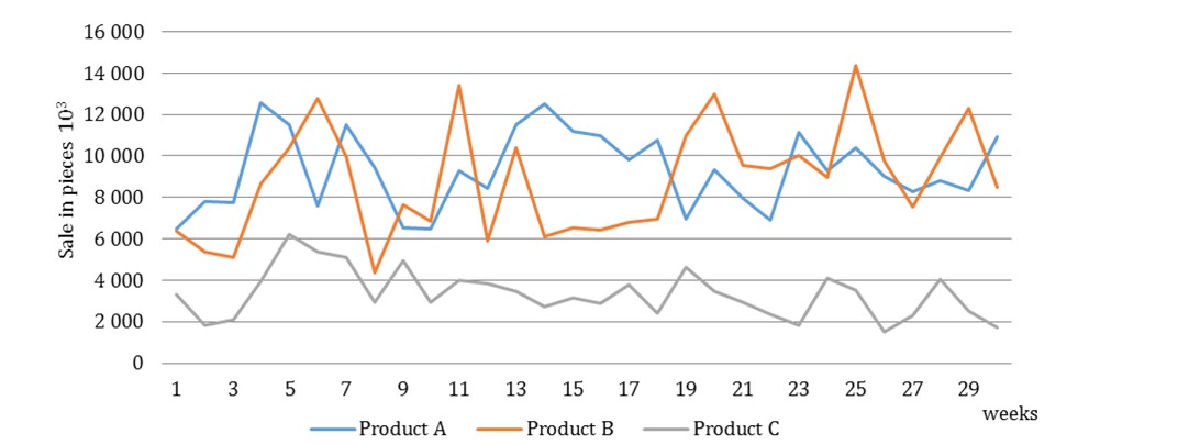
Real sales of the products A, B, C.
Demand for products A, B, C observed for 30 weeks.
| Week | Production [103 pcs] | Week | Production [103 pcs] | ||||
|---|---|---|---|---|---|---|---|
| A | B | C | A | B | C | ||
| 1 | 6,370 | 6,350 | 3,295 | 16 | 10,965 | 6,415 | 2,899 |
| 2 | 7,908 | 5,387 | 1,814 | 17 | 9,807 | 6,801 | 3,764 |
| 3 | 7,659 | 5,122 | 2,091 | 18 | 10,768 | 6,938 | 2,403 |
| 4 | 12,541 | 8,624 | 3,963 | 19 | 6,964 | 10,969 | 4,616 |
| 5 | 11,484 | 10,411 | 6,205 | 20 | 9,339 | 13,011 | 3,484 |
| 6 | 7,610 | 12,749 | 5,382 | 21 | 7,952 | 9,552 | 2,929 |
| 7 | 11,508 | 9,965 | 5,108 | 22 | 6,907 | 9,402 | 2,328 |
| 8 | 9,433 | 4,367 | 2,960 | 23 | 11,133 | 10,021 | 1,849 |
| 9 | 6,623 | 7,660 | 4,968 | 24 | 9,197 | 8,947 | 4,105 |
| 10 | 6,495 | 6,842 | 2,953 | 25 | 10,372 | 14,364 | 3,522 |
| 11 | 9,089 | 13,404 | 3,971 | 26 | 8,996 | 9,772 | 1,508 |
| 12 | 8,437 | 5,911 | 3,850 | 27 | 8,281 | 7,534 | 2,297 |
| 13 | 11,488 | 10,395 | 3,450 | 28 | 8,822 | 9,919 | 4,062 |
| 14 | 12,186 | 6,092 | 2,732 | 29 | 8,234 | 12,275 | 2,503 |
| 15 | 11,201 | 6,546 | 3,144 | 30 | 10,898 | 8,482 | 1,712 |
Entry variables related to the production of products A, B, C.
| Parameter | Unit | Value |
|---|---|---|
| Line production capacity A | ths.pcs/h | 168 |
| Line production capacity B | ths.pcs/h | 153 |
| Line production capacity C | ths.pcs/h | 173 |
| Average time of rebuilding | h | 4 |
| Price A | EUR/ths.pcs | 125 |
| Price B | EUR/ths.pcs | 118 |
| Price C | EUR/ths.pcs | 180 |
| Scrap | coeff. | 0 |
| Minimal production batch A | ths.pcs | 100 |
| Minimal production batch B | ths.pcs | 100 |
| Minimal production batch C | ths.pcs | 70 |
3 Methodology and methods
The purpose of this paper is to present two approaches to creation of a production plan for a production line. The first approach is based on forecasts and the second is based on simulations. The suitability of these approaches is compared on the basis of the selected criterion - total cost. The cost of rebuilding the line and the cost of storing finished production is considered to be the total cost.
When designing a production plan proposal, we use these two approaches:
The first approach utilizes quantitative forecasting. On the basis of the time series data analysis, the demand forecast for the production cycle time period and input raw material supply cycle, i.e. 2 and 6 weeks, is calculated. It is assumed to enter production in 1-week intervals in a volume based on a 2-week forecast. The level of safety inventory of finished products is on the level of 80% of the maximum difference of the 6-week forecast and actual sales. Total costs consist of the line breakdown costs (value of unprocessed production) and storage costs of finished production (1). An extra group of costs is the cost of safety stock. These are not dependent on production intervals and are maintained at a constant level of 80% of maximum forecast deviation from actual sales (2).
Where: CT is total cost, C hPi is capacity per hour for i-th product, Pi is price for i-th product, TR is average time for line rebuild in hours, ni is number of rebuilds for the monitored period, Bi is batch size for i-th product, m is number of products, CSF is safety cost based on forecasts, ᐃQi is maximum deviation of 2-week forecast and sales for i-th product, and F i is sales forecast for i-th product.
The second approach implements cost optimization method based on Harris-Wilson’s model using Monte Carlo simulations. The basis for optimization is the mathematical model of the cost function of total costs (4). The total costs consist of the cost of rebuilding the line (5) and the storage costs (6). The goal of optimization is to determine a production batch at which the total cost will be minimal. Subsequently, additional dependent parameters such as the production input interval (7) and the continuous production time (8) result from the optimal production batch. In modelling the cost function, it is considered that the consumption of the finished production is uniform and its stocks are supplemented at regular intervals by a constant volume of the production batch. The production batch is considered as the mean value for a given distribution. The production plan is at the mean value. Safety stock will be considered at the level of the difference of 1.5 times the standard deviation and the mean value. This is a level comparable to the level of safety stock when forecasting. Their value represents the cost of safety stocks (9).
Where: CRi is cost to rebuild the line for i-th product, CSi is storage cost for i-th product, Di is average demand for i-th product for the monitored period, ti is production input interval, tPi is continuous production time, CSS is safety cost based on simulation, σi is standard deviation, and meani is mean value.
The basis of Monte Carlo simulations is the definition of uncertainty for variable parameters in the form of appropriate distribution functions. In order to optimize production, decision variables and forecast variables have to be determined. Since demand is considered a key uncertain input variable, the distribution function is defined by using the FIT function of the Crystal Ball simulation tool. This feature allows, based on a specific time series, to describe the stochastic character of the variable by the most appropriate distribution function, including its statistical characteristics. The distribution functions of other variables are determined by estimation. Defined distributions for input and output variables are presented in Table 3. Optimization is done through the OptQuest software tool using Monte Carlo simulations.
Definition of input and output variables.
| Variable | Unit | Type | Statistical characteristics | Distribution function |
|---|---|---|---|---|
| Demand A | pcs | Input variable | using FIT | - |
| Demand B | pcs | Input variable | using FIT | - |
| Demand C | pcs | Input variable | using FIT | - |
| Time of line rebuild | h | Input variable | Mean 4; St. dev. 0.4 | Normal |
| Scrap rate | % | Input variable | Rate 5,000%; 90%=0,1; 10%=4,61 | Exponential |
| Production batch A | pcs | Decision variable | - | |
| Production batch B | pcs | Decision variable | - | |
| Production batch C | pcs | Decision variable | - | |
| Total costs | EUR | Forecast variable | - |
4 Results
4.1 Analysis of data time series
On the basis of time series analysis, an optimal prognostic method was selected to provide a prognosis for 2 and 6 weeks (Table 4, Figure 2-4) with min. MAPE (Mean Absolute Percentage Error) value. The ARIMA (2,0,2) was proposed as the most accurate predictive method. Prognoses were worked out only for weeks 17-30 due to the use of a sufficiently long time series (min. 15 data) to prepare the forecast. Subsequently, according to the formula (3), deviations of the forecast and demand for the determination of safety stock were evaluated. Table 4 presents the calculated forecasts and max. deviations of ᐃQi for individual products.
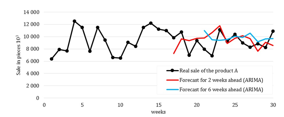
Real sale of the product A and forecasts by ARIMA.
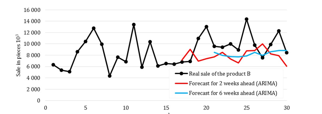
Real sale of the product B and forecasts by ARIMA.
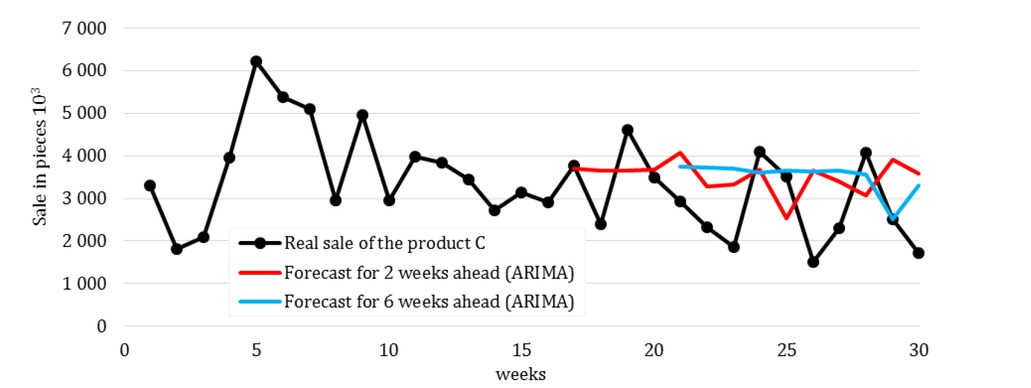
Real sale of the product C and forecasts by ARIMA.
Forecast for 2 and 6 weeks.
| Week | Forecast [103 pcs] | |||||
|---|---|---|---|---|---|---|
| A | B | C | ||||
| 2w | 6w | 2w | 6w | 2w | 6w | |
| 17 | 7,282 | 7,165 | 3,698 | |||
| 18 | 9,651 | 9,019 | 3,650 | |||
| 19 | 9,353 | 6,983 | 3,644 | |||
| 20 | 9,721 | 7,416 | 3,674 | |||
| 21 | 9,786 | 10,991 | 7,690 | 8,527 | 4,076 | 3,742 |
| 22 | 10,639 | 9,478 | 8,519 | 7,982 | 3,276 | 3,716 |
| 23 | 11,792 | 9,419 | 7,343 | 7,773 | 3,324 | 3,691 |
| 24 | 8,906 | 9,552 | 6,667 | 7,715 | 3,682 | 3,606 |
| 25 | 9,729 | 10,038 | 8,758 | 7,893 | 2,523 | 3,648 |
| 26 | 10,144 | 9,867 | 8,803 | 8,521 | 3,662 | 3,633 |
| 27 | 9,697 | 10,575 | 10,022 | 7,957 | 3,391 | 3,649 |
| 28 | 7,631 | 9,175 | 8,266 | 8,605 | 3,068 | 3,563 |
| 29 | 9,067 | 9,635 | 7,904 | 8,851 | 3,917 | 2,522 |
| 30 | 8,583 | 9,677 | 6,055 | 8,803 | 3,584 | 3,298 |
| MAPE | 17.26% | 16.75% | 25.62% | 17.04% | 47.09% | 50.82% |
| Max deviation ᐃQi | 2,525 | 5,606 | 999 | |||
4.2 Production plan based on forecasts
When planning production based on 2-week forecasts, we are considering entering the production in 7-day intervals in volume according to the forecast. This volume may be adjusted for each period either by increasing the safety stock or by reducing the overproduction from the previous cycle. Given that the volume produced is different in each period,we only consider average production over the monitored period of 30 weeks when calculating total costs. Also adjustments of production, due to replenishment of safety stock or overproduction, are not taken into account in the calculation. These deviations are offset over a longer period of time and have a negligible impact on the final cost level. The calculation of line rebuild costs and storage costs presented in Table 5 is based on formulas (5) and (6). Safety stock costs represent a value of production volume of 80% max. forecasting and sales deviations. Costs quantified in Table 5 are a period of 10 weeks.
Production costs for production planning according to forecasts.
| Costs item | For individual product [EUR] | For the whole production [EUR] |
|---|---|---|
| Line rebuild costs A | 840,000 | 2,807,760 |
| Line rebuild costs B | 722,160 | |
| Line rebuild costs C | 1,245,600 | |
| Storage costs A | 5,805,562 | 13,998,037 |
| Storage costs B | 5,196,464 | |
| Storage costs C | 2,996,010 | |
| Total costs | - | 16,805,797 |
| Safety stock value A | 252,500 | 925,485 |
| Safety stock value B | 529,188 | |
| Safety stock value C | 143,797 |
4.3 Production plan based on simulations
The distribution functions of the "sell" variable are designed through FIT function. The best functions describing sale were selected based on the chi-square test. Sales of product A optimally expressed the beta distribution, sales of product B lognormal distribution and sales of product C weibull division. Figure 5-7 present distribution functions for product sales including 1.5 standard deviation.
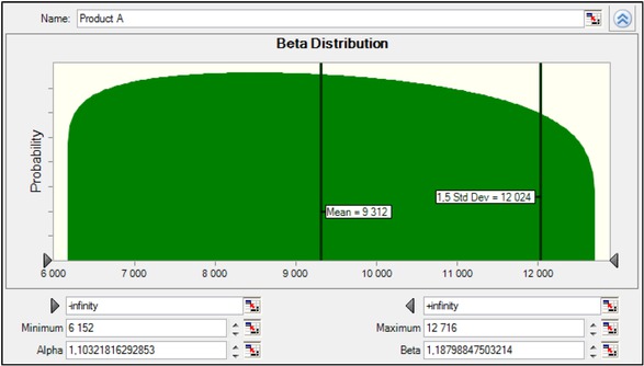
Distribution function for sale of product A.
Using OptQuest, production has been optimized with the aim to achieve a minimum mean value for forecast variable - total costs. Simulation for OptQuest was set to 10,000 trials. As shown in the graph, already at an experiment of about 1,620 the optimal solution was reached, which did not change during further simulations. Figure 8 presents the results of optimization of production, including optimal production volume. Production parameters are in Table 6 and production costs are presented in Table 7. Costs quantified in Table 7 are for a period of 10 weeks.
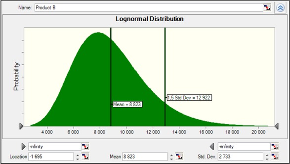
Distribution function for sale of product B.
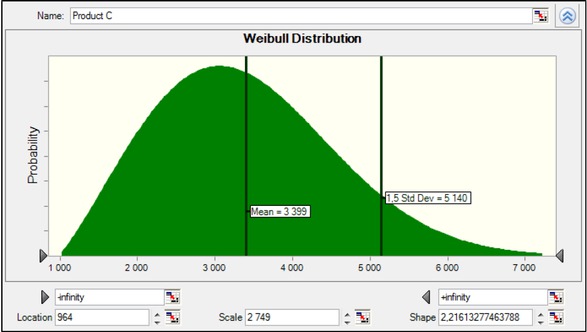
Distribution function for sale of product C.
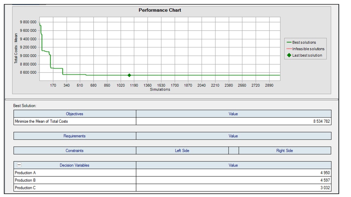
Graph of production optimization with resulting values.
Production parameters after optimization.
| Parameter | Unit | Product A | Product B | Product C |
|---|---|---|---|---|
| Production batch | pcs 103 | 4,950 | 4,957 | 3,032 |
| Interval of production input | week | 0.53 | 0.52 | 0.91 |
| Safety stock value | pcs 103 | 2,712 | 4,099 | 1,741 |
Cost of production after optimization.
| Costs item | For individual product [EUR] | For the whole production [EUR] |
|---|---|---|
| Line rebuild costs A | 1,580,218 | 4,362,626 |
| Line rebuild costs B | 1,386,038 | |
| Line rebuild costs C | 1,396,370 | |
| Storage costs A | 1,546,875 | 4,267,390 |
| Storage costs B | 1,356,115 | |
| Storage costs C | 1,364,400 | |
| Total costs | - | 8,534,782 |
| Safety stock value A | 339,000 | 1,136,062 |
| Safety stock value B | 483,682 | |
| Safety stock value C | 313,380 |
Figure 9 presents a Monte Carlo simulation histogram for Total costs. In addition to the mean value, the confidence interval is 80% is distinguished, which means that with 80% reliability it can be expected that the costs will not be less than about EUR 7,500,000 and will not exceed the level of EUR 9,600,000.
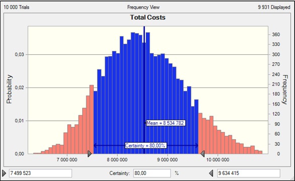
Forecast of Total costs.
Other outputs from Monte Carlo simulations allow an analysis of the impact of input variables on the output reliability. In our case study, sensitivity analysis showed that the reliability of simulation results was influenced mainly by the variability of the sale C (Figure 10). By reducing the impact of inputs variability on the output, we reduce the risk that our expected output will be different from reality. The main benefit of Monte Carlo simulation is its possible application in risk management. The identification of risk factors makes it possible to apply a selective approach in decisions about controlled variables. In our case study, there is high variability in the sale of C product, which is the strongest risk factor threatening the target by variability (Figure 10). Another strong risk factor is line rebuild time and sale of the product B.
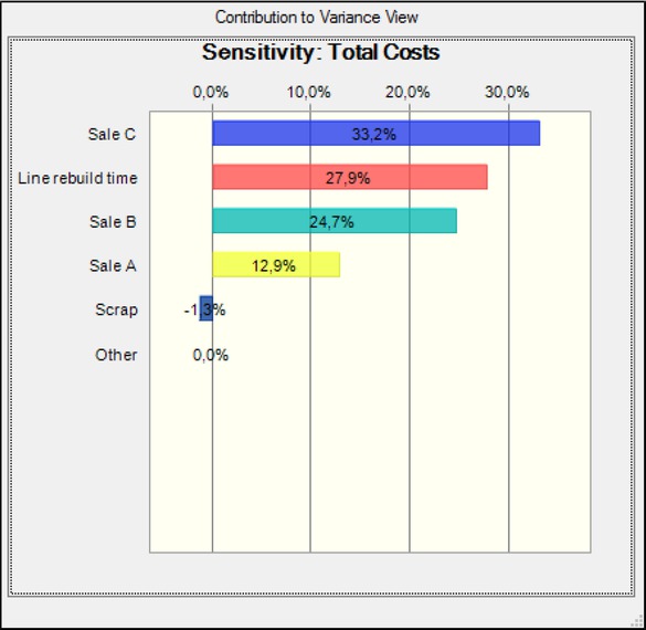
Sensitivity analysis of total costs.
5 Conclusions and future directions
Two approaches to creating an operational plan were presented in the paper. The first method used quantitative forecasting, at which based on a time series the forecast of sales for the next planning period was determined. The ARIMA (2,0,2) prognostic method was selected based on MAPE as the most reliable. Because the forecast inaccuracy required the maintenance of safety stock, in our case study, for the reason given in section 2, the safety stock was set at 80% of the maximum deviation of the forecast from reality. Production was performed at weekly intervals. Uncertainty of other input variables such as production time, line rebuild time, costs and others have not been taken into account. Costs and the amount of safety stock are presented in Table 8.
Production costs and safety stock.
| Planning method | Total costs [EUR] | Safety stock [EUR] |
|---|---|---|
| Prognoses | 16,805,797 | 925,485 |
| Simulations | 8,630,016 | 1,136,062 |
The second method applied a method of optimizing production using Monte Carlo simulations aiming to minimize costs. The stochastic character of demand was utilizing the Crystal Ball software tool captured with a suitable distribution function. Based on the estimate, the variability of the other input variables was also determined. By the means of the OptQuest, production parameters were optimized so that the total costs associated with production line rebuild and storage of finished production were minimal. Total costs and safety stock are shown in Table 8.
Production planning based on demand forecasting is always associated with the risk of low forecast accuracy. Time-series forecasting is used in planning most frequently. In production planning, where many input variables are of stochastic character, Monte Carlo simulations allow to include this stochasticity in the plan preparation, optimization and as well as to use the simulation outputs in the risk analysis. We consider this as the highest benefit of applying of Monte Carlo simulations in planning. However, there are many limitations. Also in our case study, we saw that high variability of several variables sharply reduced the plan reliability. Simulations can be used effectively in the case where input variability is low. It is important to precisely select the input variables where it is reasonable to define their stochastic character and which of them consider as constants.
Utilization of simulations and optimization by means of software tools represents an alternative to traditional approaches to production planning. The availability of software tools allows enterprises to use simulations even in such processes where quantitative prognosis is applied that requires the availability of historical data (which is not always available) and does not allow for inclusion into planning of uncertainties of other variables. Monte Carlo simulations allow to implement the uncertainty of the planned parameter (based on estimates or historical data) along with the uncertainty of other variables in the plan creation.
In the case study, we presented planning for a constant data model when data is moving within a narrow range of values. This model occurs in stabilized processes. Another character has data in unstable or cyclic processes. Therefore, further research in this area will focus on the use of simulations in production planning of products with seasonal and trend-driven demand model.
Acknowledgement
This work has been supported by grant projects VEGA 1/0708/16, VEGA 1/0063/16, VEGA 1/0638/19, KEGA 012TUKE-4/2019 and APVV SK-SRB-18-0053.
References
[1] Jeon S. M., Kim G., A survey of simulation modeling techniques in production planning and control (PPC), Prod. Plan. Control, 2016, 27(5), 360-37710.1080/09537287.2015.1128010Search in Google Scholar
[2] Ha C., Seok H., Ok C., Evaluation of forecasting methods in aggregate production planning: A Cumula-tive Absolute Forecast Error (CAFE), Comput. Ind. Eng, 2018, 118, 329–33910.1016/j.cie.2018.03.003Search in Google Scholar
[3] de Oliveira E. M., Cyrino Oliveira F. L., Forecasting mid-long term electric energy consumption through bagging ARIMA and exponential smoothing methods, Energy, 2018, 144, 776–78810.1016/j.energy.2017.12.049Search in Google Scholar
[4] Pedro H. T. C., Coimbra C. F. M., Assessment of forecasting techniques for solar power production with no exogenous inputs, Sol. Energy, 2012, 86(7), 2017–202810.1016/j.solener.2012.04.004Search in Google Scholar
[5] Ramos P., Santos N., Rebelo R., Performance of state space and ARIMA models for consumer retail sales forecasting, Robot. Comput. Integr. Manuf., 2015, 34, 151–16310.1016/j.rcim.2014.12.015Search in Google Scholar
[6] Siregar B., Nababan E. B., Yap A., Andayani U., Fahmi, Forecasting of raw material needed for plastic products based in income data using ARIMA method’, In: Proceeding - 2017 5th International Conference on Electrical, Electronics and Information Engineering: Smart Innovations for Bridging Future Technologies, ICEEIE 2017, 2018, 135–13910.1109/ICEEIE.2017.8328777Search in Google Scholar
[7] Khashei M., Hajirahimi Z., A comparative study of series arima/mlp hybrid models for stock price forecasting, Commun. Stat. Simul. Comput, 2018, 1–1610.1080/03610918.2018.1458138Search in Google Scholar
[8] Rangel-González J. A., Frausto-Solis J., Javier González-Barbosa J., Pazos-Rangel R. A., Fraire-Huacuja, H. J., Comparative study of ARIMA methods for forecasting time series of the Mexican stock exchange, In: Castillo O., Melin P., Kacprzyk J. (Eds), Fuzzy Logic Augmentation of Neural and Optimization Algorithms: Theoretical Aspects and Real Applications. Studies in Computational Intelligence, Springer, Cham, 2018, 749, 475-48510.1007/978-3-319-71008-2_34Search in Google Scholar
[9] Mircetic D., Nikolicic S.,Maslaric M., Ralevic N., Debelic B., Development of S-ARIMA Model for Forecasting Demand in a Beverage Supply Chain, Open Eng., 2016, 6(1), 407-41110.1515/eng-2016-0056Search in Google Scholar
[10] Pant M., Attri A. K., Index of industrial production: Coincident indicators and forecasting, Econ. Polit. Wkly, 2018, 53(17), 97–104Search in Google Scholar
[11] Missbauer H., Uzsoy R., Optimization Models of Production Planning Problems, In: Kempf K., Keskinocak P., Uzsoy R. (Eds.), Planning Production and Inventories in the Extended Enterprise. International Series in Operations Research & Management Science, Springer, Boston, MA, 2011, 151, 437–50710.1007/978-1-4419-6485-4_16Search in Google Scholar
[12] Sabadka D., Molnar V., Fedorko G., Jachowicz T., Optimization of Production Processes Using the Yamazumi Method, Adv. Sci. Technol. Res. J., 2017, 11(4), 175–18210.12913/22998624/80921Search in Google Scholar
[13] Huang D., Lin Z.K., Wei W., Optimal production planning with capacity reservation and convex capacity costs, Adv. Prod. Eng. Manag., 2018, 13(1), 2018, 31-4310.14743/apem2018.1.271Search in Google Scholar
[14] Lukic D., Milosevic M., Antic A., Borojevic S., Ficko M., Multi-criteria selection of manufacturing processes in the conceptual process planning, Adv. Prod. Eng. Manag, 12(2), 2017, 151-16210.14743/apem2017.2.247Search in Google Scholar
[15] Gansterer M., Almeder C., Hartl R. F., Simulation-based optimization methods for setting production planning parameters, Int. J. Prod. Econ., 2014, 151, 206–21310.1016/j.ijpe.2013.10.016Search in Google Scholar
[16] Straka M., Malindzakova M., Trebuna P., Rosova A., Pekarcikova M., Fill M., Application of EX-TENDSIM for improvement of production logistics’ efficiency, Int. J. Simul. Model., 2017, 16(3), 422–43410.2507/IJSIMM16(3)5.384Search in Google Scholar
[17] Fedorko G., Molnar V., Honus S., Neradilova H., Kampf R., The Application of Simulation Model of a Milk Run to Identify the Occurrence of Failures, Int. J. Simul. Model., 2018, 17(3), 444–45710.2507/IJSIMM17(3)440Search in Google Scholar
[18] Neradilová H. Fedorko G., The Use of Computer Simulation Methods to Reach Data for Economic Analysis of Automated Logistic Systems, Open Eng., 2016, 6(1), 700-71010.1515/eng-2016-0085Search in Google Scholar
[19] Li M., Yang F., Uzsoy R., Xu J., A metamodel-based Monte Carlo simulation approach for responsive production planning of manufacturing systems, J. Manuf. Syst., 2016, 38, 114–13310.33915/etd.6071Search in Google Scholar
[20] Soroush H., Shirouyehzad H., Performance evaluation of production companies using data envelopment analysis and Monte Carlo simulation: A case study, Int. J. Product. Qual. Manag., 2014, 13(4), 395–41310.1504/IJPQM.2014.062219Search in Google Scholar
[21] Betterton C. E., Cox J. F., Production rate of synchronous transfer lines using Monte Carlo simulation, J. Prod. Res., 2012, 50(24), 7256–727010.1080/00207543.2011.645081Search in Google Scholar
[22] Fazlollahtabar H., Es’Haghzadeh A., Hajmohammadi H., Taheri-Ahangar A., A Monte Carlo simulation to estimate TAGV production time in a stochastic flexible automated manufacturing system: A case study, Int. J. Ind. Syst. Eng., 2012, 12(3), 243–25810.1504/IJISE.2012.049410Search in Google Scholar
© 2019 J. Fabianova et al., published by De Gruyter
This work is licensed under the Creative Commons Attribution 4.0 International License.
Articles in the same Issue
- Regular Article
- Exploring conditions and usefulness of UAVs in the BRAIN Massive Inspections Protocol
- A hybrid approach for solving multi-mode resource-constrained project scheduling problem in construction
- Identification of geodetic risk factors occurring at the construction project preparation stage
- Multicriteria comparative analysis of pillars strengthening of the historic building
- Methods of habitat reports’ evaluation
- Effect of material and technological factors on the properties of cement-lime mortars and mortars with plasticizing admixture
- Management of Innovation Ecosystems Based on Six Sigma Business Scorecard
- On a Stochastic Regularization Technique for Ill-Conditioned Linear Systems
- Dynamic safety system for collaboration of operators and industrial robots
- Assessment of Decentralized Electricity Production from Hybrid Renewable Energy Sources for Sustainable Energy Development in Nigeria
- Seasonal evaluation of surface water quality at the Tamanduá stream watershed (Aparecida de Goiânia, Goiás, Brazil) using the Water Quality Index
- EFQM model implementation in a Portuguese Higher Education Institution
- Assessment of direct and indirect effects of building developments on the environment
- Accelerated Aging of WPCs Based on Polypropylene and Plywood Production Residues
- Analysis of the Cost of a Building’s Life Cycle in a Probabilistic Approach
- Implementation of Web Services for Data Integration to Improve Performance in The Processing Loan Approval
- Rehabilitation of buildings as an alternative to sustainability in Brazilian constructions
- Synthesis Conditions for LPV Controller with Input Covariance Constraints
- Procurement management in construction: study of Czech municipalities
- Contractor’s bid pricing strategy: a model with correlation among competitors’ prices
- Control of construction projects using the Earned Value Method - case study
- Model supporting decisions on renovation and modernization of public utility buildings
- Cements with calcareous fly ash as component of low clinker eco-self compacting concrete
- Failure Analysis of Super Hard End Mill HSS-Co
- Simulation model for resource-constrained construction project
- Getting efficient choices in buildings by using Genetic Algorithms: Assessment & validation
- Analysis of renewable energy use in single-family housing
- Modeling of the harmonization method for executing a multi-unit construction project
- Effect of foam glass granules fillers modification of lime-sand products on their microstructure
- Volume Optimization of Solid Waste Landfill Using Voronoi Diagram Geometry
- Analysis of occupational accidents in the construction industry with regards to selected time parameters
- Bill of quantities and quantity survey of construction works of renovated buildings - case study
- Cooperation of the PTFE sealing ring with the steel ball of the valve subjected to durability test
- Analytical model assessing the effect of increased traffic flow intensities on the road administration, maintenance and lifetime
- Quartz bentonite sandmix in sand-lime products
- The Issue of a Transport Mode Choice from the Perspective of Enterprise Logistics
- Analysis of workplace injuries in Slovakian state forestry enterprises
- Research into Customer Preferences of Potential Buyers of Simple Wood-based Houses for the Purpose of Using the Target Costing
- Proposal of the Inventory Management Automatic Identification System in the Manufacturing Enterprise Applying the Multi-criteria Analysis Methods
- Hyperboloid offset surface in the architecture and construction industry
- Analysis of the preparatory phase of a construction investment in the area covered by revitalization
- The selection of sealing technologies of the subsoil and hydrotechnical structures and quality assurance
- Impact of high temperature drying process on beech wood containing tension wood
- Prediction of Strength of Remixed Concrete by Application of Orthogonal Decomposition, Neural Analysis and Regression Analysis
- Modelling a production process using a Sankey diagram and Computerized Relative Allocation of Facilities Technique (CRAFT)
- The feasibility of using a low-cost depth camera for 3D scanning in mass customization
- Urban Water Infrastructure Asset Management Plan: Case Study
- Evaluation the effect of lime on the plastic and hardened properties of cement mortar and quantified using Vipulanandan model
- Uplift and Settlement Prediction Model of Marine Clay Soil e Integrated with Polyurethane Foam
- IoT Applications in Wind Energy Conversion Systems
- A new method for graph stream summarization based on both the structure and concepts
- “Zhores” — Petaflops supercomputer for data-driven modeling, machine learning and artificial intelligence installed in Skolkovo Institute of Science and Technology
- Economic Disposal Quantity of Leftovers kept in storage: a Monte Carlo simulation method
- Computer technology of the thermal stress state and fatigue life analysis of turbine engine exhaust support frames
- Statistical model used to assessment the sulphate resistance of mortars with fly ashes
- Application of organization goal-oriented requirement engineering (OGORE) methods in erp-based company business processes
- Influence of Sand Size on Mechanical Properties of Fiber Reinforced Polymer Concrete
- Architecture For Automation System Metrics Collection, Visualization and Data Engineering – HAMK Sheet Metal Center Building Automation Case Study
- Optimization of shape memory alloy braces for concentrically braced steel braced frames
- Topical Issue Modern Manufacturing Technologies
- Feasibility Study of Microneedle Fabrication from a thin Nitinol Wire Using a CW Single-Mode Fiber Laser
- Topical Issue: Progress in area of the flow machines and devices
- Analysis of the influence of a stator type modification on the performance of a pump with a hole impeller
- Investigations of drilled and multi-piped impellers cavitation performance
- The novel solution of ball valve with replaceable orifice. Numerical and field tests
- The flow deteriorations in course of the partial load operation of the middle specific speed Francis turbine
- Numerical analysis of temperature distribution in a brush seal with thermo-regulating bimetal elements
- A new solution of the semi-metallic gasket increasing tightness level
- Design and analysis of the flange-bolted joint with respect to required tightness and strength
- Special Issue: Actual trends in logistics and industrial engineering
- Intelligent programming of robotic flange production by means of CAM programming
- Static testing evaluation of pipe conveyor belt for different tensioning forces
- Design of clamping structure for material flow monitor of pipe conveyors
- Risk Minimisation in Integrated Supply Chains
- Use of simulation model for measurement of MilkRun system performance
- A simulation model for the need for intra-plant transport operation planning by AGV
- Operative production planning utilising quantitative forecasting and Monte Carlo simulations
- Monitoring bulk material pressure on bottom of storage using DEM
- Calibration of Transducers and of a Coil Compression Spring Constant on the Testing Equipment Simulating the Process of a Pallet Positioning in a Rack Cell
- Design of evaluation tool used to improve the production process
- Planning of Optimal Capacity for the Middle-Sized Storage Using a Mathematical Model
- Experimental assessment of the static stiffness of machine parts and structures by changing the magnitude of the hysteresis as a function of loading
- The evaluation of the production of the shaped part using the workshop programming method on the two-spindle multi-axis CTX alpha 500 lathe
- Numerical Modeling of p-v-T Rheological Equation Coefficients for Polypropylene with Variable Chalk Content
- Current options in the life cycle assessment of additive manufacturing products
- Ideal mathematical model of shock compression and shock expansion
- Use of simulation by modelling of conveyor belt contact forces