Measurement and simulation validation of numerical model parameters of fresh concrete

Ke Zhang; Wenda Yu; Dong Li; Defang Zou; Shiying Zhang

doi:10.1515/secm-2021-0042

Artikel Open Access

Measurement and simulation validation of numerical model parameters of fresh concrete

Ke Zhang , Wenda Yu , Dong Li , Defang Zou und Shiying Zhang

Veröffentlicht/Copyright: 5. August 2021

Veröffentlicht von

Veröffentlichen auch Sie bei De Gruyter Brill

Manuskript einreichen Informationen für Autor*innen

Aus der Zeitschrift Science and Engineering of Composite Materials Band 28 Heft 1

Abstract

In the numerical simulation of the macroscopic flow of the concrete, it can optimize the performance indicators of the screw conveyor and improve the uniformity of the material to be discharged in the batch production. The discrete element method is effective. The accuracy of physical parameters of this method is a key issue for the reliability of the simulation results of concrete. In this study, we measured the parameters describing the interaction between gravel, mortar, as well as between these two materials and the wall (steel). The experimentally determined parameters include the particle density, size, shape, coefficient of restitution, coefficients of static, and rolling friction. The cohesion coefficient of mortar particles for batch time was obtained by comparing the spread diameter and flow time in V-funnel experiments and simulation. After these calibration steps, the DEM parameters were validated by comparison of the mass flow rate and driving power by the batch production of screw conveying in simulations and experiments. The calculated results are proved to be close to the experimental data, which demonstrates that the measured DEM parameters are of sufficient accuracy to be used in the simulation of concrete flow performance (mass flow rate, energy consumption) in the screw conveyors.

Keywords: discrete element method; fresh concrete; model parameters; time-dependence; calibration

1 Introduction

The screw conveyor is the main equipment for the industrial production of precast concrete components, its performance directly affects the construction efficiency, cost, and quality of concrete parts. Recently, due to higher requirements of precast concrete components, an increase in the performance of screw conveyors has become an important issue to reduce costs and to accomplish intelligent and efficient operation at low waste levels. For a long, the concrete conveying process and the phenomena in the screw conveyor were difficult to understand. The discrete element method (DEM) has recently been applied extensively to gain an understanding of the internal phenomena of the screw conveyor, to control the operation. This method can provide information about the location, velocity, stress, and energy of each particle in a granular system [1,2,3]. Some researchers have used DEM to study the concrete flowability of the handling equipment (pump, screw conveyor, mixer truck) to tackle the practical problem, including discharging, mixing, segregation behaviors, and particle deposition in the pump [4,5].

In the DEM calculation, the physical parameters are principal particle properties, which affect the simulated motion of the granular matter [6]. Some of the DEM parameters are affected by shape, roughness, and size of particles [7]. Many researchers have explored the relationship between the physical parameters and the simulation results. For instance, the effects of physical parameters on the repose angle [8,9], flow time [10], and packing density (or porosity) [11,12]: all investigators found that the DEM parameters clearly affect the results, and particularly when the parameter values are varied in certain ranges.

In screw conveyor simulations by DEM, the physical parameters of concrete in different batch times (or rest times) are very different. In many DEM studies, the investigators simply used parameter values taken from the open literature in their studies without making any attempt to “measure” the parameters. There are still some investigators who use the mathematical method to determine or reduce the variation range of DEM parameters, for example, the K-means, Plackett-Burman, and Gauss-Newton iterative method [13]. If the parameters used are inappropriate, the findings of the studied parameters may be incorrect. Furthermore, the DEM parameters may be influenced not only by particle properties but also by the environment (e.g., moisture of particles and cohesion of the particles). Therefore, it is motivated to design procedures by which these DEM parameters could be “measured.”

The physical parameters can be divided into two main categories. One includes contact parameters, mainly coefficients of static and rolling friction, coefficient of restitution, and cohesion of coefficient. The other includes particle properties, e.g., particle density and size, Poisson’s ratio, and Young’s modulus. The physical parameters can be measured directly or indirectly in the experiment. For indirect measurements, Li et al. [14] described in the literature that the coefficient of friction between particles and contact wall was calibrated using a concrete standard flow test. Bouziani and Benmounah [10] stated in the literature that by measuring the flow time of concrete particles in the V-funnel, the cohesion of coefficient between particles was calibrated. According to the test of slump and expansion for concrete, the response surface optimization method is used to reverse the DEM model parameters [15]. For direct measurements, the Gaussian curve of the size distribution was measured by a particle size screening experiment in literature [16]. The volume displacement method was used to directly measure the density of rock particles in the literature [17]. The coefficient of restitution of the particles was measured with a drop test in the literature [18]. The coefficient of friction between particles and contact materials can be measured by shear experiments [19], slope experiments [20], and others.

In the current physical parameters of concrete measurement, calibration experiments are usually done at a shorter time scale rather than satisfying actual production conditions. For instance, the time-dependence of concrete resulting from the batch production mode of the screw conveyor. The physical parameter measurement in a shorter time scale is difficult to reflect the effect of the batch production mode on the parameters of the concrete DEM model. Especially, the performance of screw conveyors is influenced by the workability of concrete in batch production. Therefore, it is difficult to get the concrete physical parameters that can accurately describe the performance index of screw conveyed by the above methods. It can be seen that it not only has important theoretical significance but also has considerable practical value to establish a check method of DEM model parameters for concrete considering the influence of batch production.

Given the measurement of the physical parameters of the DEM model for concrete affected by time-dependence, it makes a systematic study for the measurement methods and results of gravel and mortar physical parameters. We first report the measurement methods and the results of determining the main physical parameters, such as particle shape, size, density, coefficient of restitution, and coefficient of static and rolling friction of gravel and mortar. Then, the coefficient of rolling friction of gravel and the coefficient of cohesion of the mortar was calibrated by comparison of the macro parameters such as the angle of repose, flow time, and spread radius of the particles built-in experiments and in simulation. At the same time, the time function of the coefficient of cohesion for mortar is fitted. Eventually, the “measured” DEM parameters are validated by comparison of the mass flow rate of concrete by the batch production of screw conveying in simulations and experiments.

2 Discrete element model of concrete

To accurately simulate the flow state of conveying concrete, an appropriate mathematical model is needed to describe the particle–particle and particle–contact wall interaction of fresh concrete. In the numerical simulation of concrete, gravel and mortar are considered as solid phases [21,22], where gravel is a non-cohesive particle and the mortar is a cohesive particle. In the DEM numerical simulation, the Hertz–Mindlin slip-free model is adopted for gravel particles [17,23]. The Johnson–Kendall–Roberts model is adopted for mortar particles [24,25]. The normal elastic contact force is calculated for the overlapping contact radius a and the coefficient of cohesion γ. In the model of fresh concrete composed of gravel and mortar, the equations of particle–particle interaction forces and moments are listed in Table 1.

Table 1

The equations of particle–particle interaction forces and moments

Force and torque	Equation
Normal elastic force, f _en,ij	− 4 π γ E ⁎ α 3 / 2 + 4 E ⁎ 3 R ⁎ α 3 , δ = − 4 π γ α E ⁎ + α 2 R ⁎
Normal damping force, f _dn,ij	− c n ( 6 m i j E ⁎ R ⁎ δ n ) 1 / 2 ν n , i j
Tangential elastic force, f _et,ij	− μ s ∣ f e n , i j ∣ ( 1 − ( 1 − δ t / δ t , max ) 3 / 2 ) δ t ˆ
Tangential damping force, f _dt,ij	− c t 6 m i j μ s ∣ f e n , i j ∣ 1 − δ t / δ t , max δ t , max 1 / 2 ν t , i j
Coulomb friction force, f _t,ij	− μ s ∣ f e n , i j ∣ δ t ˆ
Torque by tangential forces, T _ij	R i j × ( f e t , i j + f d t , i j )
Rolling friction torque, M _ij	μ r , i j ∣ f e n , i j ∣ ω ⌢ i j n

where 1 / m i j = 1 / m i + 1 / m j , 1 / R ⁎ = 1 / R i + 1 / R j , E ⁎ = E / [ 2 ( 1 − ν 2 ) ] , ω ˆ i j n = ω i j n / ∣ ω i j n ∣ , δ t = ∣ δ t ∣ , δ ˆ = δ t / ∣ δ t ∣ , R i j = R i ( r j − r i ) / ( R i − R j ) , δ t , max = μ s δ n ( 2 − ν ) / ( 2 ( 1 − ν ) ) , ν i j = ν j − ν i + ω j × R j − ω i × R i , ν n , i j = ( ν i j ⋅ n ) ⋅ n , ν t , i j = ( ν i j × n ) × n .

Note that tangential forces (f _et,ij + f _dt,ij) should be replaced by f _t,ij when δ t ≥ δ t , max .

The translation and rotation of particle–particle and particle–contact wall under the interaction are calculated by Newton’s second law. During the calculation period t, the equation of the motion of controlling particle i with mass m _i and radius R _i can be written as follows:

(1) m i d ν i d t = ∑ j = 1 k i ( f e , i j + f d , i j ) + m i g ,

(2) I i d ω i d t = ∑ j = 1 k i ( T i j + M i j ) ,

where m _i, I _i, V _i, and ω _i are the mass, moment of inertia, translational velocity, and rotational velocity of particle i, respectively, g is the acceleration due to gravity, j represents a particle i, F _e represents the elastic force, which is the summation of the normal and tangential forces F _cn,ij and F _ct,ij, respectively, at the contact point with particle j, F _d represents the damping force, which is the summation of the normal and tangential damping forces, F _dn,ij and F _dt,ij, at the contact point, T _ij and M _ij are the torque due to the tangential components of the contact forces and rolling friction torque on particle i form particle j, respectively. Moreover, I i = 2 / 5 m i R i 2 and m i = ρ × V i are the moment of the inertia and mass of the particle, respectively. The equations for the contact forces and torques in equations (1) and (2) are given elsewhere [26].

3 Measure physical parameters of the concrete

For the numerical model of gravel and mortar, physical parameters such as particle size, shape, density, the coefficient of friction, and the coefficient of cohesion have an important influence on the flowability and viscosity of simulated concrete [14]. Therefore, this section will explain the measurement methods and results of the above parameters. Among them, the Poisson’s ratio and shear modulus of gravel and mortar are obtained through literature [10,27].

3.1 Particle size and shape

The shape of the gravel is irregular and the size is random [28,29]. In this paper, the gravel particles studied were obtained from an aggregate company in China. To reduce the influence of particle size and shape on the reliability of numerical simulation, the pass rate of the particle size of the gravel was obtained through the screen test, as shown in Figure 1.

Figure 1

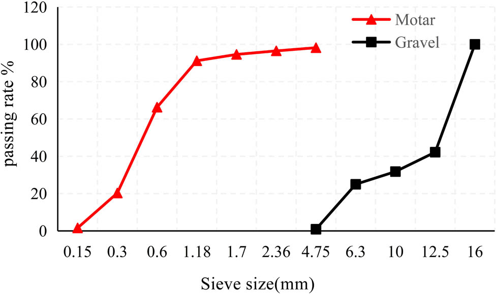
Particle size sieving pass rate.

According to the particle size distribution curve, the average value of the particle size of the gravel is 12.5 mm and the standard deviation is 2.9. To reduce the amount of calculation, three typical shapes of particles were selected through the observation method. After the three sample particles were categorized accordingly, the size of each particle was estimated using the particular shape’s DEM equivalent [2,30], as shown in Figure 2. There are many types of mortar raw materials, among which the largest particle size is the sand. By sieving the sand, it can be seen that the particle size is uniform and the maximum particle size is less than 4.75 mm. In this paper, the particle size of the mortar was uniformly set at 5 mm spherical particles [31].

Figure 2

Particle shape representation for DEM modeling of gravel. Non-spherical particles models based on a multisphere method for gravel [2].

3.2 Particle density

In order to make sure that the mass of the concrete particles in the numerical simulation is consistent with that in the experimental, the particle densities of the gravel and mortar are measured separately. Particle density is the ratio of the mass of a particle to its own volume. The density of the gravel was measured by volume displacement using a measuring cup [32]. The density of the mortar was obtained indirectly from the bulk density. When the mortar was filled with a measuring cup, the net weight of the mortar is measured as m. In this paper, the mortar model is 5 mm spherical particles, so the experiment used 5 mm glass sphere filled with measuring cup and measured the total volume of glass sphere is V = n ⋅ V 5 mm , in which n is the number of spheres and V 5 mm is the volume of a single sphere. The particle density of the mortar is calculated according to the formula ρ motar = m / V . The particle density and bulk density results of gravel and mortar are shown in Table 2.

Table 2

Density of gravel and mortar

Particle type	Diameter (mm)	Bulk density (kg/m³)	Particle density (kg/m³)
Gravel	5–15	1,425	2,591
Mortar	5	1,835	3,210

3.3 Coefficient of restitution

The coefficient of restitution is the ratio of the height of the particle before and after the collision contact material, refer Table 3. It reflects the elasticity of particles after the collision. The coefficient of restitution between gravel, mortar, and steel plates is generally measured using a drop test. The experimental device is shown in Figure 3. To reduce the statistical errors of the coefficient of restitution, the “particle plate” plane is as smooth as possible during the measurement. Meanwhile, only the motion of the particles in the vertical direction is considered in the measurement, ignoring the rotational motion. The gravel and mortar particles were randomly selected, as shown in Figure 3, each is tested 3 times, and then the average value is calculated. The results of the coefficient of restitution measurements are shown in Table 3.

Table 3

Coefficient of restitution of the particles

Particle type	Coefficient of restitution			Equation
Particle type	Steel	Gravel	Mortar	Equation
Gravel	0.1	0.05	0.04	e w = H 1 / H 2
Mortar	0.01	0.04	0.01	e w = H 1 / H 2

Note: H ₁ is the starting drop height, H ₂ is the height of the bounce after impact.

Figure 3

Measurement of the coefficient of restitution: particle plates: (1) gravel, (2) steel, (3) mortar, (4) selected particle, and (5) measuring drop height ruler.

3.4 Coefficient of friction

The coefficients of static and rolling friction are the two main parameters in the DEM model [33,34]. According to the definition of friction coefficient, the coefficient is measured by a self-made friction coefficient measuring device, as shown in Figure 4. To measure the friction coefficient between gravel, mortar and steel plate, particle plates of different materials are used, as shown in Figure 3.

Figure 4

Measurement device of the coefficient of friction: (a) three-dimensional representation of device and (b) experimental device. The upper slope rotated to the position where particles started slipping on the surface. The angle of the upper slope, the height of the particle, and the horizontal distance are measured [34]. Particle plates are shown in Figure 3.

3.4.1 Coefficient of static friction

To reduce the error caused by the rotation of the particles when measuring the static friction coefficient, the gravel and mortar balls (non-sticky) are fixed on the acrylic plate with glass glue. In the experiment, the moving speed of the slider is as low as possible to ensure that the high-speed camera can accurately capture the position where the particles start to move. The particles were placed at three different positions on the inclined surface and the experiment was repeated 5 times. After removing the abnormal value in the result, the average value and dispersion are obtained. Table 4 summarizes the value of the static friction coefficient.

Table 4

Coefficient of static friction of gravel and mortar

Particle type	Means value of the coefficient of static friction			Equation
Particle type	Steel	Gravel	Mortar	Equation
Gravel	0.43	0.47	0.52	μ s = tan θ
Mortar	0.18	0.52	0.25	μ s = tan θ

Note: The standard deviation of the coefficient of static friction of the gravel is 0.05 and the mortar is 0.043.

3.4.2 Coefficient of rolling friction

To reduce the influence of particle shape and surface roughness on the measurement results, the gravel particles with smooth surface and nearly spherical shape were screened. The particles were placed at three different positions on the inclined surface and the experiment was repeated 5 times. After removing the abnormal value in the result, the average value and dispersion are obtained. Table 5 summarizes the value of the rolling friction coefficient. See the literature for a detailed derivation of the formula [34].

Table 5

Coefficient of rolling friction of gravel and mortar

Particle type	Means value of the coefficient of rolling friction			Equation
Particle type	Steel	Gravel	Mortar	Equation
Gravel	0.08	0.1	0.13	μ r = h / d
Mortar	0.06	0.13	0.08	μ r = h / d

Note: The standard deviation of the coefficient of static friction of the gravel is 0.037 and the mortar is 0.03.

The rolling friction coefficient of the above-mentioned measured particles is an idealized case, ignoring the errors caused by the shape and surface roughness of the particles. The angle of repose experiment was carried out on the gravel, to correct the error of rolling friction coefficient during the measurement. By adjusting the rolling friction coefficient, make sure that the simulation values of the angle of repose are in agreement with the experimental values. The device consists of a slump cone and a spread length tester, as shown in Figure 5(a). The slump cone is filled with gravel particles, and it is quickly lifted after the particles piled up smoothly. The particles collapsed and accumulated on the spread diameter tester (steel plate) to form a stable angle of repose.

Figure 5

Schematic diagram of slump and v-funnel test (a–b), experimental instrument diagram (c).

3.5 Coefficient of cohesion

The bonding property of mortar directly affects whether the mortar can effectively coat the gravel particles, thereby affecting the workability of the concrete. The cohesion coefficient of the mortar particles is mainly used to simulate the cohesion of the mortar macroflow. By comparing the flow time of the V-funnel experiment and simulation, the methods are used to calibrate the cohesion coefficient of mortar particle–particle [35]. The cohesion coefficient of the particles and the contact wall is calibrated by the self-compacting spread diameter after the mortar flows. The V-funnel experiment is repeated every 10 min, recording the discharge time and self-compacting spread diameter of mortar on the time scale. The device is shown in Figure 5(b), and the experimental results are shown in Figure 6.

Figure 6

Discharge time and spread diameter with different batch time through V-funnel experiment for mortar.

It can be seen that as the batch time scale increases, the mortar discharge time from the V-funnel becomes longer and the cohesion becomes stronger. In contrast, the self-compacting spread diameter of the mortar on the Spread tester decreases, and the deformability of the mortar is also decreased. This is the macroscopic flow change rule of mortar. According to this rule, in the numerical simulation of the V-funnel experiment, the combination of the cohesion coefficients of mortar particle–particle and particle–contact wall is modified so that the discharge time and the self-compacting spread diameter are consistent with the trend of experimental results. Another purpose is to reduce the measurement error of the above parameter through the correction of the cohesive coefficient of mortar.

The calibration process of the above parameters will affect the measurement efficiency and accuracy, so that they cannot be determined by a single experiment, but requires a certain logical order. Since the coefficients of friction and cohesion interact, and the particle model parameters are idealized in the measurement. Therefore, the measurement errors are revised in the determination of the last parameter such as the coefficient of cohesion for mortar particles and the coefficient of rolling friction for gravel particles. The steps to determine the model parameters are shown in Figure 7.

Figure 7

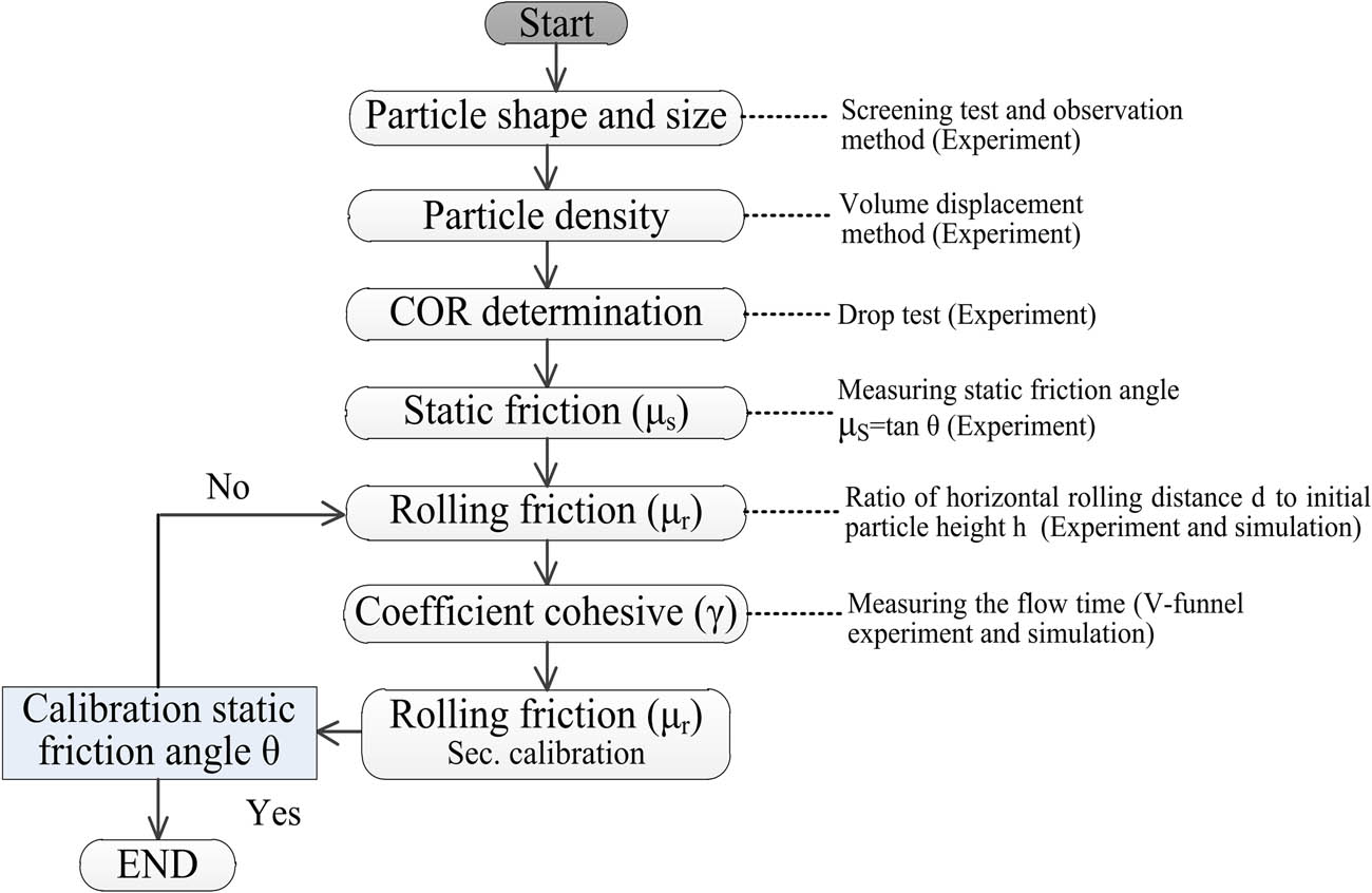
DEM parameter verification process of particles.

4 Result and discussion

Based on the physical parameters of the gravel and mortar in the experiment, by contrast with the angle of repose, the discharging time, and spread diameter experimental and simulation value, verify the reliability of the DEM model for the gravel and mortar, respectively. At the same time, the time function of the coefficient of cohesion of mortar is fitted in the DEM simulation. The calibrated physical parameters of concrete were used to analyze the flow performance of different batch processes for screw conveyors. And the DEM model of concrete was proved by comparing the mass flow rate of the simulation result with the measured result.

The simulations were calculated on a desktop computer whose CPU, RAM, and GPU are 3.7 GHz (Inter Xeon 6126), 64 GB, and NVIDIA P4000, respectively. The discharge process for V-funnel took 20 process seconds and the simulation finished within 40 h for each case. The simulation contained 87,000 particles. The slump process for the cone took five process seconds and the simulation finished within 4 h for each case. The simulation contained 2,800 particles. The discharge process for the screw conveyor took 15 process seconds and the simulation finished within 45 h for each case. The simulation contained 88,000 particles.

4.1 Research on slump cone test of gravel

The experimental results of physical parameters of gravel are used for numerical simulation of the collapse process of gravel in the slump cone. The DEM model parameters are corrected by comparing the simulation values and experimental values of the angle of repose and spread diameter.

When measuring the angle of repose, the image processing method is used to collect the image of the piled-up shape of the gravel from the horizontal direction [36,37]. Then, the boundary contour of the image is processed by using MATLAB and fits the coordinate data, the results are shown in Figure 8(a). According to the fitted linear equations, the angle of repose of simulation and experiment are solved, which are 14.1° and 17.6°, respectively, and the error is 19.8%. The spread diameter is measured directly with a ruler to obtain simulation and experimental results of 498 and 442 mm, respectively, with an error of 11.2%. This is mainly due to the selection of relatively smooth particles to measure the coefficient of rolling friction. While the actual gravel is polygonal and angular with rough surface particles, thus, it makes the measurement result error relatively large.

Figure 8

Fitting results of the angle of repose for gravel (a) and simulation and experimental diagram of repose angle (b).

Taking the experimental measurement results of the angle of repose and the spread diameter as the target values, a single variable method is used to modify the rolling friction coefficient of the particle–particle and particle–contact wall. The variation curves of the obtained angle of repose and the spread diameter are shown in Figure 9. It can be seen from the figure that as the rolling friction coefficient increases, the angle of repose increases while the spread diameter decreases. According to the slope of the linear fitting equation, the rolling friction coefficient from particle–particle is more sensitive to the angle of repose and the spread diameter than the particle–contact wall. Therefore, in the numerical simulation, the rolling friction coefficient from particle–particle is preferentially determined, and then the particle–contact wall is fine adjusted. When the rolling friction coefficients of the particle–particle and particle–contact wall are 0.1 and 0.08, respectively, the maximum error between the angle of repose and spread diameter obtained from the simulation and the measurement result is 6.4%, as shown in Figure 8(b). Therefore, the shape and surface roughness of the gravel have a great influence on the measurement of the rolling friction coefficient of the particles and cannot be ignored.

Figure 9

Variation curve of rolling friction coefficient, angle of repose, and spread diameter.

4.2 Research on V-funnel experiment of mortar

Without considering the effect of time-dependence on the physical properties of the mortar, the parameters measured experimentally are called preliminary parameters. The numerical simulation of the discharging of mortar from the V-funnel is carried out based on the mortar model parameters. The timing starts when the funnel outlet is opened, and the mortar particles flow out until it is empty, and the timing ends. The relationship between the cohesion coefficient of mortar particles and the emptying time, self-compacting expansion diameter is shown in Figure 10.

Figure 10

Variation curves of cohesion coefficient, discharge time, and spread diameter.

It can be seen from Figure 10 that as the cohesion coefficient of the mortar particles increases, the discharge time increases and the self-compacting spread diameter decreases. To reduce the calibration workload of the cohesion coefficient, the change interval of the coefficient of cohesion for the particle–particle and particle–contact wall was first determined in the simulation. Then the cohesion coefficient was fine-tuned so that the mortar of the discharging time and self-compacting spread diameter has consistency on the experimental measurement results. When the coefficient of cohesion of particle–particle and particle–contact wall for the mortar are r _pp = 0.25j and r _pw = 0.15j, respectively, the emptying time is 3.2 s and the self-compacting spread diameter is 608 mm. It can be considered that parameters can accurately describe the mortar (T _rest = 5 min) macroscopic flow.

To further verify the model parameters, the mortar was filled into the slump cone freely, and the average bulk density was 1,886 kg/m³ in simulation, and the experimental measurement result was 1,835 kg/m³, with an error of 2.7%. This slight error is due to the magnification of the mortar particle size in the simulation so that there is porosity between the particles. For cohesive materials such as mortar, the above calibration method will reduce the workload. At the same time, because the parameters of the mortar model are idealized in the measurement, the resulting errors are compensated in the calibration of the cohesion coefficient.

4.2.1 Time function of cohesion coefficient of mortar

According to the V-funnel test results in Section 3.5, the batch time causes the discharging time to increase and the self-compacting deformability to decrease, which indicates that the cohesion of mortar gradually increases. To simulate the change of macroscopic flow of mortar, the cohesion coefficient at T _rest = 5 is taken as the benchmark, and the cohesion coefficient is modified so that the measured average mass flow rate and self-compacting spread diameter are close to the experimental values at different batch times. The simulation and experiment of mortar flow through the V-funnel at different batch times are shown in Figure 11(a)–(c).

Figure 11

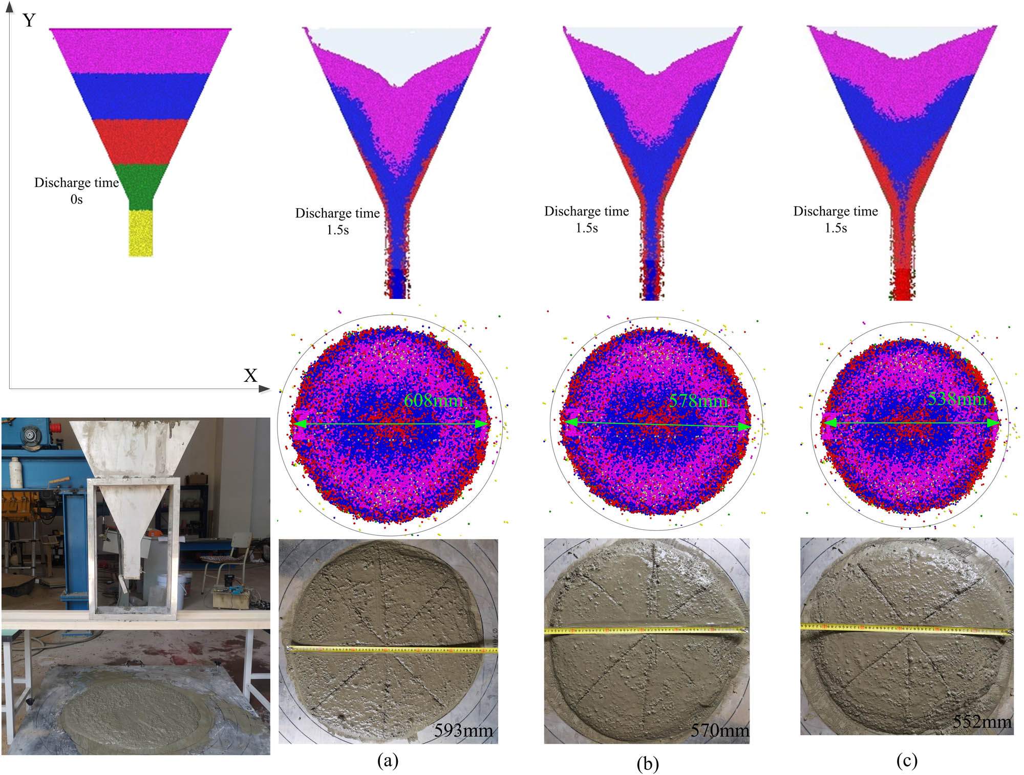
Snap-shots of discharging concrete in V-funnel experiment (bottom) and the DEM simulation (top) for the different batch times: (a) 5 min, (b) 15 min, and (c) 25 min.

As shown in Figure 11, with the increase of the batch time, the number of mortar particles remaining in the V-funnel increases at the same discharge time (1.5 s), that is, it becomes difficult for the mortar to flow in the funnel. In addition, the spread diameter of the mortar on the spread tester is getting smaller and smaller, and the numerical simulation of mortar flow through the V-funnel is consistent with the macroflow index measured by experiments. Therefore, the modified cohesion coefficient of mortar can be used to predict the macroscopic flow under the influence of time dependence.

According to the V-funnel experiment results, the variation of the cohesion coefficient with the batch time is calibrated, as shown in Figure 12. It can be seen that the variation gradient of the cohesion coefficient for the particle–particle is higher than that of the particle–contact wall. Through data fitting for the cohesion coefficient of mortar, the time function of the cohesion coefficient was derived in the paper.

Figure 12

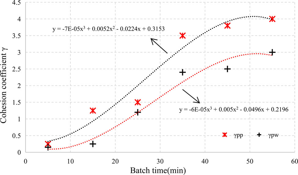
Variation of the cohesion coefficient at different batch times.

4.2.2 Verification of physical parameters of mortar

In order to verify the DEM model parameters of the mortar particles, the average mass flow rate and the self-compacting spread diameter at different batch times through the V-funnel simulation are compared with the experiment values. The average mass flow rate is the ratio of mortar mass to discharge time, Mass avg = Mass funnel / t emptying . Figure 13 shows the change of the average mass flow rate with the batch time. It can be seen that the average mass flow rate decreased with increasing batch time. The trend of the simulation value is consistent with the experimental value, with a maximum error of 7.1%.

Figure 13

Average mass flow of mortar at different batch times.

The self-compacting spread diameter mainly describes the deformability of the mortar. The mortar was freely discharged into the spread tester in the V-funnel test until equilibrium conditions exist. The value of self-compacting spread diameter in the horizontal and vertical is measured and the average value is obtained. Figure 14 shows that as time increases, the spread diameter decreases. All these suggest that the deformability of the mortar becomes worse. The simulation prediction value of the self-compacting spread diameter is consistent with the experimental value and the maximum error is 4.4%. The results prove that the combination of experiment and simulation can be used to calibrate the cohesion coefficient of concrete. And finally, the strategy of calibrating the cohesion coefficient can effectively compensate the measurement error of other parameters in the experiment.

Figure 14

Self-compacting spread diameter of mortar under different batch times.

4.3 Screw conveying concrete in the batch process

Concrete discharging is typically handled using a screw conveyor. The flow characteristics of concrete particles depend upon raw materials, ratio, environmental factors, and physical properties. The batch production of screw conveyors is the main cause of the time-dependent performances of fresh concrete. Especially, the time-dependent performances of fresh concrete will directly affect the design parameters (mass flow rate, energy consumption) of the screw conveyor in the casting process. And all this owed to affect the quality and cost of the precast concrete. By using theoretical analytical and experimental methods, the mechanism of screw conveying concrete and particles flow behaviors cannot realize the visual analysis at the mesoscale. In addition, the traditional analytical model cannot describe the influence of concrete property changes on conveying volume. The discrete element method is an effective method, which was used to simulate the performance of screw conveyors and concrete casting.

The objectives of this section were to (1) verify that the calibrated physical parameters of concrete can accurately describe the macro flow performance of different batch processes for DEM simulation and (2) based on the DEM method, evaluate the feasibility of applying screw conveying concrete in batch process.

4.3.1 Experimental setup

In this article, a model screw conveyor was built to investigate the mass flow rate of concrete and the energy consumption in different batch times. The screw conveyor configuration used here is a laboratory-scale one. It is assumed that the concrete particles’ movement behavior is in conformity with industrial production. The 3D geometric model is shown in Figure 15(a). The key dimensions of the hopper, screw channel, and the parameters of the screw are annotated in the figures. The experimental device is shown in Figure 15(b). The concrete is filled into the hopper, and the concrete is discharged into the bucket at the set speed. During discharge, the mass of concrete within the bucket was measured by a load cell (in kg/s). The current (mA) and voltage (V) values of the motor are measured by a digital multimeter. In the numerical simulation of concrete discharging, periodic boundary conditions are applied to the DEM of the screw conveyor. By counting the mass of concrete from the discharge port and the driving power per unit time, the simulation value of the mass flow rate and driving power has been obtained.

Figure 15

The 3D geometric model of screw conveyor (a) and the experimental equipment (b). It consists of nine parts: screw conveyor (A); controller (B and C); screw (D); motors (E); power (F); plowshare mixer (G); scale (H); and guide plate (I).

4.3.2 Results

In the DEM model, the concrete was discharged following the experimental procedures in different batch times. The flow patterns of concrete can be observed in simulation. Figure 16 shows the flow of concrete out of the discharge port for the hopper. There is a good agreement between the DEM and experimental results in the continuous discharging. To further verify the physical parameters of concrete with different batch times, by comparing the experimental value and simulation value of the mass flow rate and driving power, the error was calculated, and the result is shown in Figure 17.

Figure 16

Concrete discharging behavior in the screw conveyor experiment (left) and the DEM (right).

Figure 17

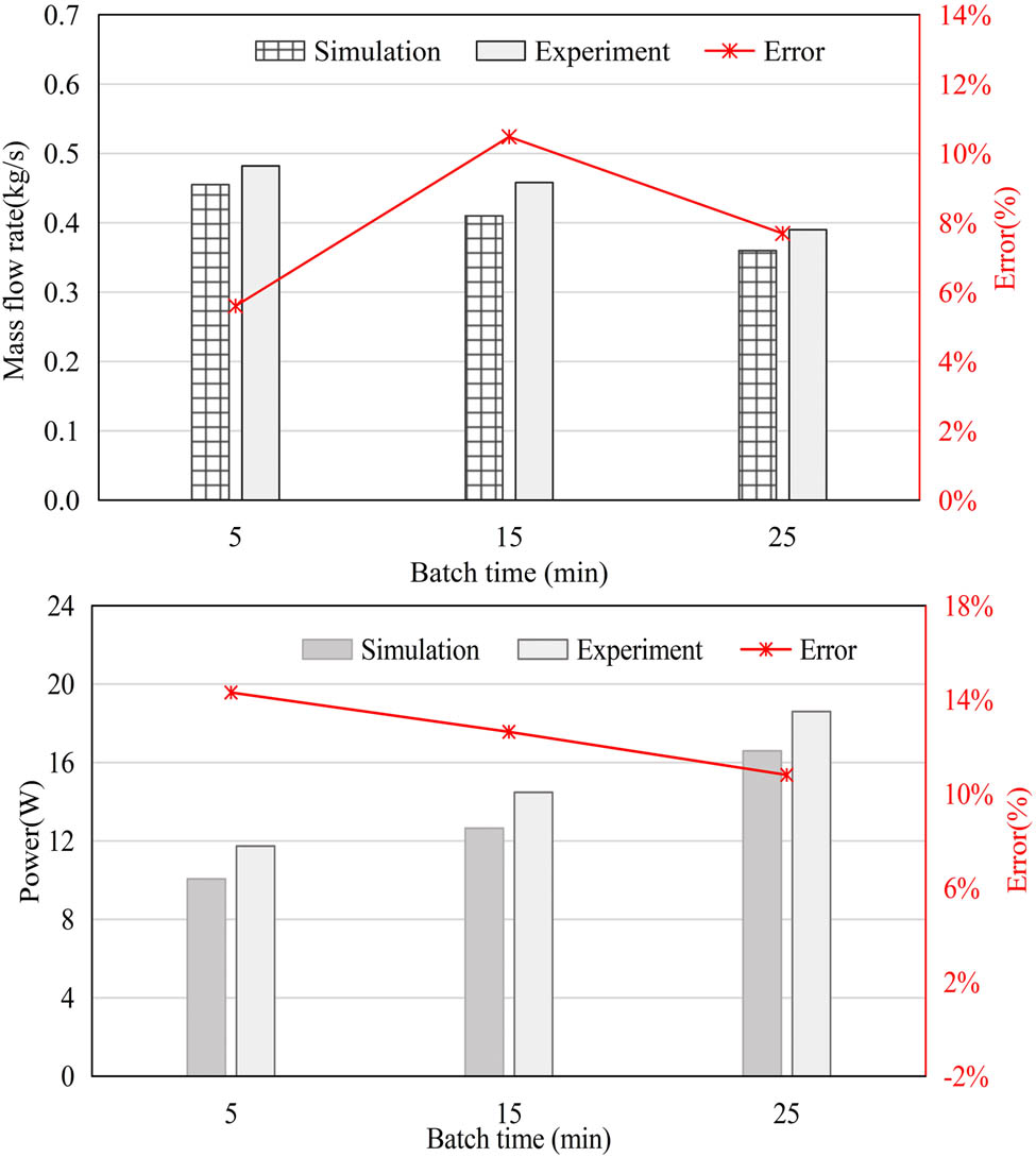
Influence of concrete flow characteristics on mass flow rate and driving power (batch time: 5–25 min, screw pitch: 40 mm, flight diameter: 60 mm, core diameter: 24 mm, rotate speed 30 rpm).

With the increase of batch time, the mass flow rate of concrete decreases and the driving power of the screw increases. The experimental value of the performance index for the screw conveyor (mass flow rate, driving power) was bigger than the simulation value in the same conditions. At the same time, the simulation values were basically consistent with the experiment data. And the maximum error of mass flow rate was not more than 10.5%, the maximum error of driving power was not more than 14.3%. The results showed that the physical parameters of mortar and gravel can accurately describe the flow performance of concrete in batch production. The error reason is that the prolonged batch time made the cohesion of concrete enhance, resulting in less concrete filled into the screw flight within the same time. In addition, with the increase in the viscosity of concrete, the torque of the screw blade to overcome the cohesion and friction of particles increases. Therefore, the typical material of concrete has a serious time dependence, which has seriously affected the mass flow and energy consumption under batch production.

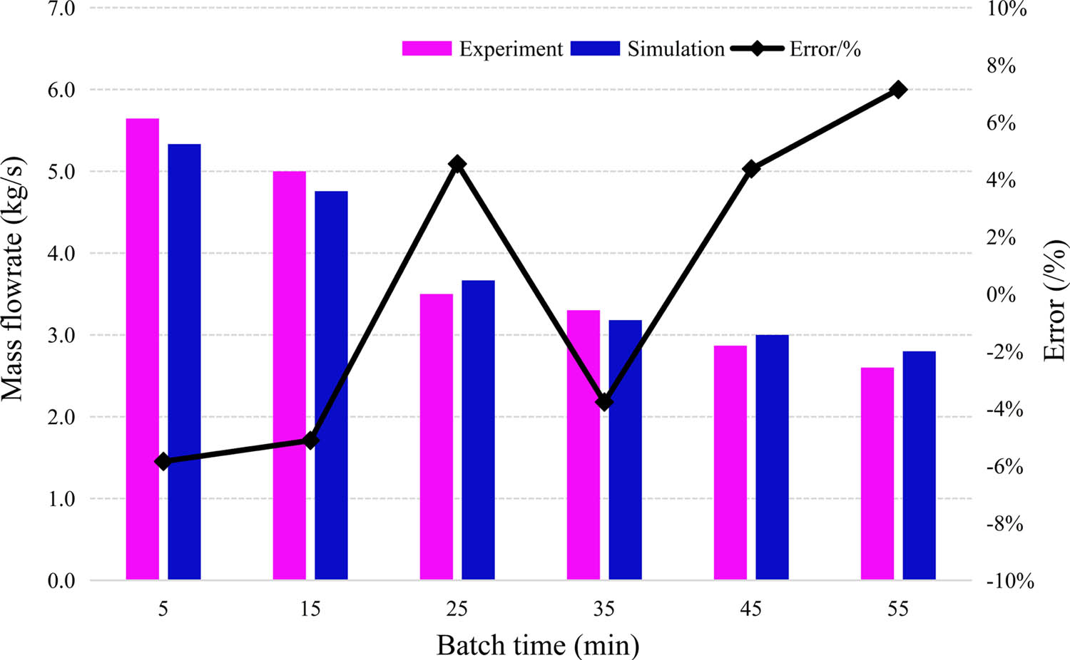
To evaluate the feasibility of the concrete DEM model and physical parameters in predicting the performance index of screw conveyor in the batch process, the mass flow rate and the driving power are predicted by randomly selecting from the different batch times (10 min, 30 min) of concrete in simulation. According to the time function of the cohesive coefficient of mortar particles in Section 4.2, the corresponding coefficient is calculated to simulate concrete discharging. Figure 18 shows the curve of the mass flow rate of concrete with the discharging time. The figure shows that with the increase in the discharging time, the mass flow rate rises sharply, and then tends to be quasi-static. Meanwhile, in the process of continuous discharging, the instantaneous values of mass flow rate have a certain degree of discreteness. This is because that the deposition effect for concrete, which makes the proportion of gravel filled into the screw flight volume has a certain degree of randomness. In addition, the mean value of mass flow rate for concrete in batch time (10 min) is bigger and steady compared to the batch time (30 min) under the same operating conditions. Obviously, the increase of batch time can cause the flowability of concrete to become lower. Meanwhile, the volumetric efficiency of the screw is smaller and the porosity of concrete is bigger. By comparing the mass flow rate of the DEM predicted value with the experimental value, it can be seen that there has been the same change trend with discharge time. The maximum error of mass flow rate (mean value) is less than 8.3%.

Figure 18

Influence of concrete flow characteristics on mass flow rate at different batch times: (a) 10 min and (b) 30 min.

Figure 19 shows the curve of driving power for screw conveying concrete with discharging time. The figure shows that the friction and cohesive forces between concrete particles need to be overcome when the screw begins to shear motion. The instantaneous values of power rapidly increase, and the growth rate is approximately linear. When the concrete is discharged continuously and stably, the driving power tends to be quasistatic from peak values. When the screw blade is in contact with the large particle or particle clusters, there has a phenomenon of carton. Meanwhile, the curve shows that the anomalous peak values of power, as shown in Figure 19. In addition, the driving power of the screw for the concrete (batch time 30 min) is larger than the concrete (batch time 10 min) in the same condition. This is because that the increase of batch time can cause the viscosity of concrete to become stronger, and the blade shear action on overcoming the moment of resistance of material becomes bigger. By comparing the DEM predicted value of power with the experimental value, it can be seen that there has been the same change trend with discharge time. The maximum error of power (mean value) is less than 10.07%. The results demonstrated that the concrete DEM model and physical parameters can accurately predict the performance index of the screw conveyor with batch production.

Figure 19

Influence of concrete flow characteristics on driving power at different batch times: (a) 10 min and (b) 30 min.

By numerically simulating the screw conveying concrete in different batch times, the given nonlinear power function fitting the relationship between the performance index of the screw conveyor (mass flow rate, power) and batch time. The function equations of mass flow rate and driving power are as follows:

Mass flowrate = 0.646 x − 0.185 ( Adj . R 2 = 0.9 ) and

Driving power = 5.416 x 0.343 ( Adj . R 2 = 0.93 )

for concrete (the batch time is less than 55 min).

The regressions were significant at the 95% confidence level. The equation of performance index can be applied to the control system of the screw conveyor to achieve the real-time control of discharging weight. According to the DEM model and physical parameters of concrete, the equation of performance index under different process parameters will be further fitted to improve the prediction accuracy and reliability.

5 Conclusion

In DEM numerical simulation, the physical parameters of the particles play a decisive role in the accuracy of the simulation prediction results. Some key parameters of two main burden materials (gravel and mortar) in the screw conveying process were measured directly or indirectly in this work. To accurately simulate the flow of concrete in the screw conveyor during the batch production process, the coefficient of cohesion for mortar in different batch times was obtained. The methods and conclusion can be highlighted as follows:

A particle experiment is an effective method to evaluate concrete materials and estimate the physical parameters of the DEM model. The verification process and sequence of parameter has a significant impact on measurement efficiency and accuracy.

The shape and surface roughness of gravel have a significant influence on the measurement accuracy of friction coefficient, and the angle of the repose experiment is an effective method to correct and verify the coefficient of friction.

Under the influence of time-dependent change characteristics of mortar, the cohesion coefficient is a function of time rather than a constant. In the V-funnel test, the discharging time and the self-compacting spread diameter of the mortar are the effective indexes for calibrating the cohesion coefficient.

Concrete conveying experiments were carried out to verify the accuracy of the measured DEM parameters. The experimental and simulation results of the mass flow rate and driving power showed good consistency, which demonstrates that the measured DEM parameters are accurate enough to be used in simulations of more complex conditions encountered in different batch production of the screw conveying process.

Acknowledgements

I would like to thank all those author who helped me to concise my paper. Ke Zhang, who put forward many valuable suggestions to my paper. Other authors give a lot of help in experiments and translation. Thank you for the financial support of the National Key R&D Program (2017YFC0704003) and the Liaoning Provincial Department of Education Project (Z2219050). On the one hand, solve the problem of experimental equipment, on the other hand, purchase relevant raw materials. Thank you for the support given to the experimental site by the Ministry of Housing and Urban-Rural Development Project (2019-K-079) and Liaoning Provincial Department of Science and Technology Project (20180551119).

Funding information: This research was financially supported by the National Key R&D Program (2017YFC0704003); Ministry of Housing and Urban-Rural Development Project (2019-K-079); Liaoning Provincial Department of Science and Technology Project (20180551119); and Liaoning Provincial Department of Education Project (Z2219050).
Conflict of interest: The author declares no conflict of interest.

References

[1] Fernandez JW, Cleary PW, Mcbride W. Effect of screw design on hopper drawdown of spherical particles in a horizontal screw feeder. Chem Eng Sci. 2011;66:5585–601.10.1016/j.ces.2011.07.043Suche in Google Scholar

[2] Zhan Y, Gong J, Huang Y, Shi C. Numerical study on concrete pumping behavior via local flow simulation with discrete element method. Materials. 2019;12:1–21.10.3390/ma12091415Suche in Google Scholar PubMed PubMed Central

[3] Yu WD, Zou DF, Dong L. Development of a new intelligent concrete spreading technology. Bull Transilvania Univ Brasov. 2018;11:217–22.Suche in Google Scholar

[4] Dong L, Peng Z, Fan LT. Research on multi-agent control system for concrete distribution, 3rd China-Romania Science and Technology. Sem Mater Sci Eng. 2018;399:1–6.10.1088/1757-899X/399/1/012029Suche in Google Scholar

[5] Tan YQ, Deng R. Numerical study of concrete mixing transport process and mixing mechanism of truck mixer. Eng Comput. 2015;32:1041–65.10.1108/EC-04-2014-0097Suche in Google Scholar

[6] Wei H, Hao N, Ying L. Measurement and simulation validation of DEM parameters of pellet, sinter and coke particles. Powder Technol. 2020;364:593–603.10.1016/j.powtec.2020.01.044Suche in Google Scholar

[7] Chen Z, Yu J, Xue D. An approach to and validation of maize-seed-assembly modelling based on the discrete element method. Powder Technol. 2018;14:333–49.10.1016/j.powtec.2017.12.007Suche in Google Scholar

[8] Zhang X, Li Z, Zhang Z. Discrete element analysis of the rheological characteristics of self-compacting concrete with irregularly shaped aggregate. Arab J Geosci. 2018;11:294–314.10.1007/s12517-018-3960-1Suche in Google Scholar

[9] González MC, Fuentes JM. Determination of the mechanical properties of maize grains and olives required for use in DEM simulations. J Food Eng. 2012;111:553–62.10.1016/j.jfoodeng.2012.03.017Suche in Google Scholar

[10] Bouziani T, Benmounah A. Correlation between v-funnel and mini-slump test results with viscosity. KSCE J Civ Eng. 2013;17:173–8.10.1007/s12205-013-1569-1Suche in Google Scholar

[11] Zhou ZY, Zou RP, Pinson D. Dynamic simulation of the packing of ellipsoidal particles. Ind Eng Chem. 2011;50:287–91.10.1021/ie200862nSuche in Google Scholar

[12] Hamzah M. A review on the angle of repose of granular materials. Powder Technol. 2018;330:397–417.10.1016/j.powtec.2018.02.003Suche in Google Scholar

[13] Lan Q, Liu C, Cui W. Calibration of contact parameters of DEM for fresh self-compacting concrete. J Funct Mater. 2018;7:7050–6.Suche in Google Scholar

[14] Li Z, Cao G, Tan Y. Prediction of time-dependent flow behaviors of fresh concrete. Constr Build Mater. 2016;125:510–9.10.1016/j.conbuildmat.2016.08.049Suche in Google Scholar

[15] Zhang K, Yu T, Yu W, Zou D. Calibration of concrete discrete element parameters based on JKR bond model. Concrete. 2020;8:46–55.Suche in Google Scholar

[16] Stahl M, Konietzky H. Discrete element simulation of ballast and gravel under special consideration of grain-shape, grain-size and relative density. Granul Matter. 2011;13:417–28.10.1007/s10035-010-0239-ySuche in Google Scholar

[17] Horn E. The calibration of material properties for use in discrete element models. Stellenbosch: Stellenbosch University; 2012.Suche in Google Scholar

[18] Wang L, Zhou W, Ding Z, Li X. Experimental determination of parameter effects on the coefficient of restitution of differently shaped maize in three-dimensions. Powder Technol. 2015;284:187–94.10.1016/j.powtec.2015.06.042Suche in Google Scholar

[19] Liu J, Yun B, Zhao C. Identification and Validation of Rolling Friction Models by Dynamic Simulation of Sandpile Formation. Int J Geomech. 2012;12:484–93.10.1061/(ASCE)GM.1943-5622.0000156Suche in Google Scholar

[20] Wang L, Li R, Wu B. Determination of the coefficient of rolling friction of an irregularly shaped maize particle group using physical experiment and simulations. Particuology. 2018;38:1034–46.10.1016/j.partic.2017.06.003Suche in Google Scholar

[21] Deng R, Tan YQ, Zhang H. Numerical study on the discharging homogeneity of fresh concrete in truck mixer: Effect of motion parameters. Part Sci Technol. 2016;2:146–53.10.1080/02726351.2016.1227409Suche in Google Scholar

[22] Cundall PA, Strack ODL. A discrete numerical model for granular assemblies. Geotechnique. 1979;29:47–65.10.1680/geot.1979.29.1.47Suche in Google Scholar

[23] Kuan X, Bai MH. DEM simulation of particle descending velocity distribution in the reduction shaft furnace. Metall Res Technol. 2016;113:603–19.10.1051/metal/2016035Suche in Google Scholar

[24] Yang M, Li S, Yao Q. Mechanistic studies of initial deposition of fine adhesive particles on a fiber using discrete-element methods. Powder Technol. 2013;248:44–53.10.1016/j.powtec.2012.12.016Suche in Google Scholar

[25] Johnson KL, Kendall K, Roberts AD. Surface energy and contact of elastic solids. Proc R Soc A. 1971;324:301–13.10.1098/rspa.1971.0141Suche in Google Scholar

[26] Dheeraj M, Abhishek S. A review of granular flow in screw feeders and conveyors. Powder Technol. 2020;366:369–81.10.1016/j.powtec.2020.02.066Suche in Google Scholar

[27] Remond S, Pizette P. A DEM hard-core soft-shell model for the simulation of concrete flow. Cem Concr Res. 2014;58:169–78.10.1016/j.cemconres.2014.01.022Suche in Google Scholar

[28] Coetzee CJ. Review: calibration of the discrete element method. Powder Technol. 2017;310:104–42.10.1016/j.powtec.2017.01.015Suche in Google Scholar

[29] Barrios GKP, Carvalho RM, Kwade A. Contact parameter estimation for DEM simulation of iron ore pellet handling. Powder Technol. 2013;248:84–93.10.1016/j.powtec.2013.01.063Suche in Google Scholar

[30] Shi C, Shen J, Xu W, Wang R. Micromorphological characterization and random reconstruction of 3D particles based on spherical harmonic analysis. J Cent South Univ. 2017;24:1197–206.10.1007/s11771-017-3523-8Suche in Google Scholar

[31] Grima AP, Wypych PW. Development and validation of calibration methods for discrete element modelling. Granul Matter. 2011;13:127–32.10.1007/s10035-010-0197-4Suche in Google Scholar

[32] Höhner D, Wirtz S, Scherer V. Experimental and numerical investigation on the influence of particle shape and shape approximation on hopper discharge using the discrete element method. Powder Technol. 2013;235:614–27.10.1016/j.powtec.2012.11.004Suche in Google Scholar

[33] Chung YC, Liao HH, Hsiau SS. Convection behavior of non-spherical particles in a vibrating bed: Discrete element modeling and experimental validation. Powder Technol. 2013;237:53–66.10.1016/j.powtec.2012.12.052Suche in Google Scholar

[34] Ketterhagen WR, Bharadwaj R, Hancock BC. The coefficient of rolling resistance(CoRR) of some pharmaceutical tablets. Int J Pharmaceutics. 2010;392:107–10.10.1016/j.ijpharm.2010.03.039Suche in Google Scholar PubMed

[35] Attachaiyawuth A. Effect of powder type viscosity modifying agent on flowability of self-compacting mortar. J Thail Concr Assoc. 2019;7:22–9.Suche in Google Scholar

[36] Peilin L, Mustafa U. A new approach for the automatic measurement of the angle of repose of granular materials with maximal least square using digital image processing. Comput Electron Agric. 2020;172:1–10.10.1016/j.compag.2020.105356Suche in Google Scholar

[37] Tiejun L, Xuewen W, Bo L. Parameter optimization of coal particle model based on discrete element method. China Powder Technol. 2018;24:12–8.Suche in Google Scholar

Received: 2021-03-25

Revised: 2021-07-06

Accepted: 2021-07-15

Published Online: 2021-08-05

This work is licensed under the Creative Commons Attribution 4.0 International License.

Artikel in diesem Heft

https://doi.org/10.1515/secm-2021-0042

Schlagwörter für diesen Artikel

discrete element method; fresh concrete; model parameters; time-dependence; calibration

Creative Commons

BY 4.0