A hard-core soft-shell model for vibration condition of fresh concrete based on low water-cement ratio concrete

Xiaotian Li; Guangnian Xie; Zhurui Gao; Chuxin Wang

doi:10.1515/secm-2021-0057

Article Open Access

A hard-core soft-shell model for vibration condition of fresh concrete based on low water-cement ratio concrete

Xiaotian Li , Guangnian Xie , Zhurui Gao and Chuxin Wang

Published/Copyright: December 31, 2021

Published by

Become an author with De Gruyter Brill

Submit Manuscript Author Information

From the journal Science and Engineering of Composite Materials Volume 28 Issue 1

Abstract

The newly developed vibration-compacting modular production technology of concrete with low water-cement ratio puts forward new requirements for the study of rheological mechanical model of concrete. The existing contact model of discrete element method cannot effectively express the complex dynamic relationship between concrete aggregate and mortar under vibration. In this article, an improved hard-core soft-shell contact model, which is suitable for the simulation of concrete with low water-cement ratio under vibration state, is proposed according to the vibration and compactness characteristics of the concrete. According to the rheological properties of the concrete mortar, the calculation method of soft-shell force is improved. The relationship between the shear stress and its displacement in the process of trying to solve the tangential soft-shell is clarified. In order to characterize the adsorption effect of mortar on aggregate, the gravitation is added in the normal soft-shell force calculation. Slump test under non-vibration state and L-box test under vibration state are carried out to verify the correctness of the improved hard-core soft-shell contact model. The improved hard-core soft-shell contact model can effectively simulate the dynamic response of the complex multiphase concrete fluids with low water-cement ratio, and accurately characterize the change in its rheological properties.

Keywords: hard-core soft-shell model; HI theory; shear-vibration equivalent theory; PFI parameters

1 Introduction

Under the background of building industrialization, adopting the new low water-cement ratio concrete vibration compaction modular production instead of the traditional high water-cement ratio concrete casting process can effectively reduce energy consumption and improve production efficiency. Low water-cement ratio concrete is a kind of discontinuous material [1]. Mortar is a non-Newtonian fluid, and coarse aggregate shows the property of discrete particles [2]. In the process of concrete flow, there is a very complex dynamic relationship between the components [3]. The traditional computational fluid dynamics method cannot analyze it. With the development of digital simulation technology, the technology is gradually widely used in the research of concrete characteristics. Gram and Silfwerbrand [4] divided concrete simulation methods into three categories: Discrete element method (DEM), Computational fluid dynamics, and the combination of DEM and computational fluid dynamics.

The DEM was originally proposed by Cundall and Strake [5] for the simulation of rock particles. Noor and Uomoto [6] used DEM to simulate concrete first and established a simulation model based on DEM. Concrete was divided into two parts: aggregate and mortar. Aggregate and mortar were represented by different sizes of particles, and different characteristics of aggregate and mortar were represented by different parameters. On the basis of previous studies, Chu and Machida [7] improved the original DEM model and proposed a modified DEM model. They believed that concrete was two-phase material, in which the aggregate was the core of round particles and the mortar was the bonding layer wrapped around the aggregate. The characteristics of the concrete are characterized by analyzing the interaction between the bond and the mortar. Cui et al. [8] used irregular particles as aggregate, and further analyzed the influence of particle size distribution on the flow performance of the concrete.

All the above studies used trial and error method to determine the parameters of the model, but the simulation results were affected by multiple parameters, and different parameter combinations may produce the same simulation results [9,10]. The mapping relationship between the model parameters and the rheological parameters of the concrete was established. Shyshko and Mechtcherine [11,12] put forward a DEM model suitable for concrete, and used this model to simulate the slump of the concrete. Combined with the simulated normal extrusion force curve and the theoretical curve of stress distribution, the mapping relationship between normal bond strength and yield stress was established. Zhang et al. [13] established the positive interaction constitutive relationship between the concrete particles to simulate the flow process of the concrete. Li et al. [14] established the slump model of concrete by using the DEM, measured the contact parameters between particles in the specific DEM model, and described the flow process of concrete in the slump test. Zhao et al. [15] established a new dynamic coupling discrete element contact model, studied different concrete, and verified the correctness of DEM model according to the results of the concrete rheological test.

Remond and Pizette [16] proposed the hard-core soft-shell model, and considered that concrete was composed of soft-shell made of mortar and hard-core made of aggregate. Bingham model [17] was used to calculate the tangential force between the particles. In order to verify the correctness of the model, the slump test was carried out. The test showed that the model could better explain the characteristics of the concrete. However, on the one hand, the characteristics of low water-cement ratio concrete are discontinuous, which is difficult to be analyzed by the traditional computational fluid dynamics, and the existing hard-core soft-shell model cannot model the rheological behavior of low slump. On the other hand, the different excitation parameters will affect the rheology of low water-cement ratio concrete, and the change in rheology will greatly affect the compaction effect of the concrete under excitation. Therefore, the key to solve the selection of excitation parameters is to study the rheology of concrete under excitation conditions. At present, there is lack of theoretical research on the rheology of low water-cement ratio concrete under excitation, and the existing theoretical models cannot analyze the rheology of concrete under excitation.

The research on the test methods of concrete working performance can be traced back to the 1920s. So far, there are many test methods to evaluate the working performance of concrete. Most test methods comprehensively evaluate the working performance of concrete by measuring the fluidity of concrete mixture, adding other performance test methods or combined with observation experience [18]. L-box test is a device proposed by Billberg to test the fluidity and gap carrying capacity of self- compacting concrete [19]. Nguyen et al. [20] studied the relationship between L-box test and rheological parameters of the homogeneous concrete. They believed that when the vertical baffle of L-box was opened in an instant, its final shape was the result of the joint action of rheological parameters and inertia of the concrete. When the vertical baffle was opened slowly, the final shape of L-box test only depends on the yield stress of the concrete.

In this article, concrete is divided into two phases: mortar and coarse aggregate. Round particles are used to represent the hard-core of the coarse aggregate. Mortar is regarded as a soft-shell wrapped in particles. Based on the hard-core soft-shell model proposed by Remond and Pizette [16], the calculation method of soft-shell force in the model is improved, and the discrete element model of low water-cement ratio concrete under non-vibration and vibration states is established and the model is verified by slump test and L-box test.

2 Basic theory

2.1 Hard-core soft-shell model

The hard-core soft-shell model is proposed by Remond and Pizette to simulate the rheological behavior of the concrete [16]. This section briefly summarizes the hard-core soft-shell model, and puts forward the limitations of the model under vibration.

2.1.1 Model assumptions

As shown in Figure 1, according to the composition of the concrete, the concrete is divided into coarse aggregate and mortar [16]. The coarse aggregate is abstracted as a round particle, referred to as “hard-core,” and the mortar is abstracted as a concentric adhesion layer wrapped outside the coarse aggregate, referred to as “soft-shell.”

Figure 1

Schematic diagram of hard-core soft-shell model assumption.

Under the above assumptions, the hard-core phase is used to characterize the physical properties of the coarse aggregate, the interaction between hard-cores is called “hard-core force,” the soft-shell phase is used to characterize the rheological properties of the mortar, and the interaction between the mortar and particles is called “soft-shell force.” The interaction between the two particles is the superposition of hard-core force and soft-shell force.

(1) F = F hc + F ss ,

where F hc is the hard-core force and F ss is the soft-shell force.

2.1.2 Calculation of hard-core force

The hard-core force can be divided into normal component and tangential component.

(2) F hc = F hc n + F hc t ,

where F hc n is the normal hard-core force and F hc t is the tangential hard-core force.

The normal hard-core force can be calculated by the nonlinear Hertz model, and the calculation formula is shown in equation (3).

(3) F hc n = − 2 3 E R ¯ ξ n 3 / 2 + γ n E R ¯ ξ n ξ ̇ n n 12 ,

where ξ n is the overlap of normal hard-core and its unit is m. γ n is the normal damping coefficient and its unit is s. n 12 is the normal unit vector. R ¯ is the equivalent radius and its unit is m, and the calculation formula is shown in equation (4). E is the equivalent stiffness and its unit is Pa, and the calculation formula is shown in equation (5).

(4) R ¯ = r 1 r 2 r 1 + r 2 ,

(5) E = Y 1 − v 2 ,

where r 1 , r 2 are the radius of the hard-core, as shown in Figure 2. Y is Young’s modulus and its unit is Pa. v is Poisson’s ratio.

Figure 2

Schematic diagram of hard-core soft-shell model.

The tangential hard-core force can be calculated according to Mindlin–Deresiewicz theory, and the formula is shown in equation (6).

(6) F hc t = μ ∣ F hc n ∣ 1 − 1 − ∣ ξ t ∣ ξ max 3 / 2 t 12 ,

where μ is the friction coefficient. ξ t is the cumulative tangential displacement and its unit is m. t 12 is the tangential unit vector. ξ max is the maximum tangential displacement and its unit is m. ξ max can be calculated by equation (7).

(7) ξ max = ξ n μ 2 − v 2 ( 1 − v ) .

The above model is called Hertz-Mindlin model, which can effectively characterize the interaction between solid particles.

2.1.3 Calculation of soft-shell force

Similar to the hard-core force, the soft-shell force can be divided into normal soft-shell force and tangential soft-shell force.

(8) F ss = F ss n + F ss t .

Remond and Pizette [16] simplified the normal soft-shell force as a spring model. In order to ensure a large amount of overlap between the soft-shell forces, normal soft-shell forces are generated only when the distance between the hard-cores is less than a specific value h min . The normal soft-shell force is usually taken as h min = w m / 2 . w m is the thickness of the soft-shell and its unit is m. The calculation formula of the normal soft-shell force is shown in equation (9).

(9) F ss n = k ss n ( r 1 + r 2 + h min − d 12 ) n 12 , ( r 1 + r 2 + h min − d 12 ) ≥ 0 0 , ( r 1 + r 2 + h min − d 12 ) < 0 .

The tangential soft-shell force can be calculated according to Bingham model.

(10) F ss t = S ( τ 0 , m + μ m γ ̇ ) ,

where S is the contact area of the soft-shell, and its size is π r s 2 . r s is the radius of the contact surface and its unit is m. τ 0 , m is the yield stress of mortar and its unit is Pa. μ m is the plastic viscosity of mortar and its unit is Pa s. γ ̇ is the shear rate and its unit is m/s, and the calculation formula is shown in equation (11).

(11) γ ̇ = 2 v 1 , 2 , t max ( d 12 − r 1 − r 2 , h max ) ,

where v 1 , 2 , t is the tangential relative velocity, and the calculation formula is shown in equation (12).

(12) v 1 , 2 , t = v 1 r 1 r 1 eq 2 − v 2 r 2 r 2 eq 2 + r 1 eq ω 1 r 1 r 1 eq 2 + r 2 eq ω 2 r 2 r 2 eq 2 × n 12 ,

where r 1 eq and r 2 eq are the equivalent soft-shell radii as shown in the Figure 2 and its unit is m. The calculation formulas are shown in equations (13) and (14). ω 1 and ω 2 are the angular velocities of the particles and its unit is rad/s.

(13) r 1 eq = d 12 2 + ( r 1 + w m ) 2 − ( r 2 + + w m ) 2 2 d 12 ,

(14) r 2 eq = d 12 − r 1 eq ,

where d 12 is the hard-core spacing as shown in Figure 2 and its unit is m.

2.1.4 Limitations of the model

The hard-core soft-shell model establishes the relationship between DEM model parameters and rheological parameters of the mortar. At the same time, the simplification of the model greatly reduces the simulation time. However, this model still has the following problems:

The tangential soft-shell force does not consider the case that the shear stress is less than the yield stress. When the external force is not applied and the tangential velocity is 0, the particles still receive tangential soft-shell force whose magnitude is S × τ 0 , m . This situation is contrary to the physical properties of the concrete.
The normal soft-shell force does not consider the repulsive force between the particles. In the simulation, the particles repel each other, which lead to a large number of particles separated from each other. Therefore, it cannot be used in the simulation of low water-cement ratio concrete.
The rheological parameters in the model are fixed, so it is impossible to analyze the rheological characteristics of the concrete under vibration.

2.2 Shear-vibration equivalent theory

Hattori-Izumi (HI) theory and modified HI theory are only applicable to concrete in shear state [21,22,23]. When concrete is subjected to vibration, HI theory and its modification cannot characterize vibration effect. To solve this problem, a shear-vibration equivalent theory [24] is proposed, which converts the vibration intensity into the shear rate. Combined with the modified HI theory, the rheological properties of the cement slurry and mortar under vibration condition can be calculated. The following are a brief summary of the shear-vibration equivalent theory.

Figure 3 shows the flow field in vibration state [25], and the shear rate can be calculated by equation (15).

(15) γ ̇ A,B = ( v A − v B ) / d r ,

where v A and v B are the velocities of A and B, respectively, and d r is the distance between A and B. The velocity vector is divided into i and j directions, where i is perpendicular to the current flow field plane and j is perpendicular to the line between A and B. Thus, the shear rate can be expressed by equation (16).

(16) γ ̇ A,B = ( v A , i − v B , i ) i d r + ( v A , j − v B , j ) j d r ,

where v A , i and v B , i are the relative velocities of A and B in i direction; v A , j , v B , j are the relative velocities of A and B in j direction.

Figure 3

Flow field distribution of rotary viscometer in vibration state.

Combined with the shear-vibration equivalent theory, the shear action of fluid can be expressed as follows.

(17) γ ̇ total = γ ̇ vibration + γ ̇ shear ,

where γ ̇ total represents the shear rate at any point in the flow field. γ ̇ vibration represents the shear rate caused by the vibration. γ ̇ shear represents the shear rate caused by the rotation of the rotary viscometer rotor.

For unidirectional vibration, it is difficult to characterize the shear rate caused by harmonic motion. Based on the modified HI theory, a new parameter γ ̇ vib is introduced to represent the shear rate caused by vibration. Meanwhile, since the vibration can be approximately generated only along the z axis, equation (17) can be simplified as follows.

(18) γ ̇ total = γ ̇ vib 2 + γ ̇ shear 2 .

Combining with the modified HI theory, memory module Γ and flocculation rate H can be transformed as follows.

(19) Γ ( r , z , t ) = ∫ 0 t α ( t − t ′ ) γ ̇ total ( r , z , t ′ ) d t ′ ,

(20) H ( γ ̇ , t ) = K ( t ) γ ̇ total 2 + l , t > 0 H ( γ ̇ total 2 , 0 ) = k 1 ( 1 − U 0 ) 4 l , t = 0 ,

where, α is a memory function, which is used to characterize the influence of the past state on the current viscosity. K ( t ) is the empirical function and its unit is 1/s³. l is the empirical constant and its value is identically equal to 1/s². U 0 is the average number of reversible bonding of a single cement particle at t = 0.

The viscosity of the Bingham fluid should also be expressed by γ ̇ total .

(21) η = τ γ ̇ = τ 0 γ ̇ total + μ ,

where η is apparent viscosity and its unit is Pa s. τ 0 is the initial yield stress and its unit is Pa. μ is the actual viscosity of cement paste and its unit is Pa s.

3 Improvement in hard-core soft-shell model

Aiming at the shortcomings of the hard-core soft-shell model and according to the rheological properties of the mortar, the calculation method of soft-shell force is improved.

3.1 Improvement in calculation method of tangential soft-shell force

When the shear stress of Bingham fluid is greater than the yield stress, Bingham fluid behaves as viscous fluid, and the shear stress is linearly related to the shear rate. When the shear stress is less than the yield stress, Bingham fluid behaves as an elastic body, and the shear stress is proportional to the tangential displacement. The formula is as follows [17].

(22) τ = τ 0 , m + μ m γ ̇ , τ ≥ τ 0 , m G γ , τ < τ 0 , m ,

where τ is the shear stress and its unit is Pa. G is the shear modulus of the fluid material and its unit is Pa. γ is the tangential strain.

According to the above fluid characteristics, the calculation method of tangential soft-shell force is improved by author, and the calculation formula is shown in equation (23).

(23) τ = S ( τ 0 , m + μ m γ ̇ ) , τ ≥ τ 0 , m k ss t ξ t , τ < τ 0 , m ,

where, k ss t is the tangential soft-shell stiffness and its unit is N/m. ξ t is the tangential cumulative displacement and its unit is m.

In order to consider the attenuation of velocity in mortar, Remond multiplied a series of scaling coefficients such as r 1 r 1 eq 2 and r 2 r 2 eq 2 ; however, this calculation method has the following problems.

As shown in Figure 4, the soft-shell of the particles pass through the hard-core of the particles, which leads to r 1 < r 1 eq and r 1 r 1 eq 2 > 1 . The velocity of soft-shell in the mortar is enlarged, which goes against the actual situation. When the distance between the two particles is small enough, r 1 eq decreases to 0, and then the scaling coefficient r 1 r 1 eq 2 tend to infinity, resulting in excessive tangential soft-shell force and divergence of simulation.

Figure 4

Special case of soft-shell passing through hard-core.

In order to solve the above problems, the calculation method of tangential relative velocity is simplified. Because the thickness of soft-shell is relatively small, the attenuation of velocity in mortar is small and it can be ignored. In this case, the calculation method of tangential relative velocity can be modified as follows.

(24) v 1 , 2 , t = v 1 − v 2 + ( r 1 eq ω 1 + r 2 eq ω 2 ) × n 12 .

3.2 Improvement in calculation method of normal soft-shell force

Shyshko and Mechtcherine [11] adopted two motion modes of the upper particles to carry out the test. One is that the upper particles are far away from and close to the lower particles at a constant speed. The other is to make the upper particles move intermittently at the position set in the test. By simplifying the test curve, the normal force contact model of the concrete particles is established, as shown in Figure 5. When the particles are far away from each other, their normal gravity increases to a limit value, which is defined as the normal bond strength of the particles by Shyshko. Mechtcherine and Shyshko [12] further simplified the above model, ignoring the repulsion force of the particles when they are close to each other, and established a new normal force contact model of the concrete particles, as shown in Figure 6. Mechtcherine and Shyshko [12] thought that the rising slope of normal force is equal to the stiffness of collision when the normal force is less than the yield force.

Figure 5

Normal force contact model of Shyshko and Mechtcherine [11].

Figure 6

Normal force contact model of Mechtcherine and Shyshko [12].

Considering that the concrete moves violently under the condition of vibration, the overlapping of particles should be considered. In this article, the calculation method of normal soft- shell force is improved.

As shown in Figure 7, when the hard-core spacing is less than 0, the normal force is calculated by Hertz-Mindlin model. When the hard-core spacing is greater than 0, the particles are subjected to normal soft-shell force, which is composed of elastic component and viscous component.

(25) F ss n = F ss , e n + F ss , d n ,

where F ss , e n is the elastic component of normal soft-shell force and its unit is N. F ss , d n is the viscous component of normal soft-shell force and its unit is N. The viscous component of normal soft-shell force is calculated by equation (26).

(26) F ss , d n = − c ss n v 12 , t ,

where c ss n is the damping coefficient of normal soft-shell and its unit is kg/s.

Figure 7

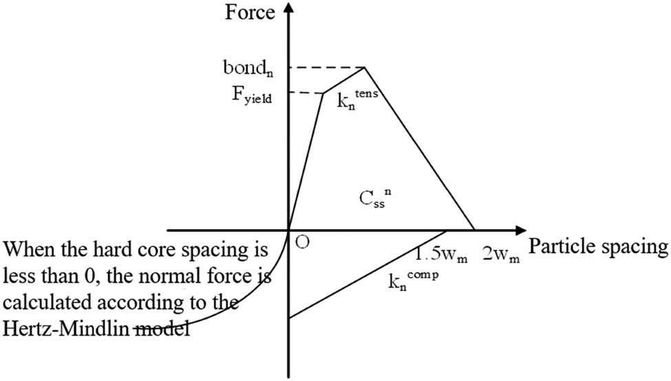
Improvement of normal force displacement curve.

When the particles are far away from each other, the calculation of elastic component of normal soft-shell force is shown in equation (27).

(27) F ss , e n = k n init δ n n 12 , 0 ≤ δ n ≤ F yield k n init k n tens δ n + F yield 1 − k n tens k n init n 12 , F yield k n init < δ n ≤ δ bond ( − k n desc δ n + 2 w m k n desc ) n 12 , δ bond < δ n ≤ 2 w m ,

where δ n is the hard-core spacing between the particles and its unit is m. k n init is the stiffness of the soft-shell at the initial far away stage and its unit is N/m, and the calculation formula is given in equation (28). δ bond is the core distance when the normal soft-shell force reaches the normal bond strength bond n and its unit is m. Its calculation formula is shown in equation (29). F yield is the yield force, which is generally taken as F yield = 0.9 bond n . k n tens is the stiffness of the second rising stage of normal soft-shell force and its unit is N/m. k n desc is the stiffness of the normal soft-shell at the stage of force reduction and its unit is N/m, and the calculation formula is given in equation (30).

(28) k n init = E R ¯ ,

(29) δ bond = bond n k n tens − F yield k n init − k n tens k n init k n tens ,

(30) k n tens = bond n 2 w m − δ bond .

When the particles are close to each other, in order to ensure enough overlap of particles, considering that the elasticity of normal soft-shell force is small, the elastic force of normal soft-shell is calculated only when the hard-core spacing between particles is less than 1.5 w m . The calculation formula is as follows.

(31) F ss , e n = ( k n comp δ n − 1.5 w m k n comp ) n 12 , 0 ≤ δ n < 1.5 w m 0 , δ n ≥ 1.5 w m ,

where k n comp is the extrusion stiffness of normal soft-shell force and its unit is N/m.

3.3 Parameter updating under vibration state

According to HI theory and Wallevik’s subsequent research [21,22,23], vibration destroys the internal structure of concrete and changes the rheological properties of the concrete. Combined with the shear-vibration equivalent theory, the effect of vibration on the concrete can be equivalent to that of shear rate. And the yield stress determines bond n . Therefore, combined with the shear-vibration equivalent theory and the modified HI theory, the rheological parameters of the concrete under vibration conditions, i.e., yield stress and viscosity, can be updated to construct the concrete DEM contact model suitable for vibration state.

Combined with the calculation characteristics of DEM, it is necessary to use discrete method to calculate each calculation formula in the modified HI theory. The specific model parameter flow is as follows.

The simulation step size of the system is determined;
The shear rate and flocculation rate of the soft-shell at the current time are calculated;
Update α and β memory functions;
According to the updated memory function, the memory modulus is updated;
Update model viscosity μ and τ ;
According to the relationship between yield stress and normal bond strength in equation (33), bond n parameters are updated.

The above process can simulate the concrete under vibration state through continuous iteration.

4 Test verification and analysis

In order to verify the correctness of the improved model, the slump test and L-box test under vibration state are simulated, and the accuracy of the simulation results is verified by the test results.

4.1 Simulation verification of slump test

The purpose of slump test [16] is to check the workability of the newly made concrete, so as to check the difficulty in concrete flow. In this section, the improved hard-core soft-shell contact model is used for slump simulation test in PFC3D software. The parameters of the contact model are set as shown in Table 1 according to the Remond test conditions. In the simulation process, the particle parameters are set as shown in Table 2.

Table 1

Parameters of slump test simulation model

Model parameter	Y	v	μ	γ n	μ m	k ss t	k n tens	k n comp	c ss n
Unit	Pa	—	—	N s/m	Pa s	N/m	N/m	N/m	N s/m
Value	2.6 × 10⁹	0.3	0.5	0.0702	10	100	200	50	1.0

Table 2

Particle parameter setting of slump test

Model parameter	Thickness of soft-shell	Hard-core radius	Density
Unit	m	m	kg/m³
Value	0.002	0.006	2,300

For the improved soft-shell hard-core contact model proposed in this article, the normal bond strength bond n and yield stress τ 0 , m play a major role in the simulation. Therefore, this article only changes the values of the above two parameters to study the influence of normal bond strength and yield stress on the simulation results. Because the mapping relationship between normal bond strength and yield stress is unknown, it is necessary to calibrate the mapping relationship between normal bond strength and yield stress. Combined with the relationship between the maximum shear stress of concrete elements and the concrete height proposed by Murata [26], as shown in equation (32), the yield height of concrete h 0 can be obtained, where the maximum shear stress of the concrete is equal to the yield stress of the concrete. According to the improved hard-core soft-shell contact model, the simulated force distribution curve is fitted, as shown in Figure 8. Mechtcherine and Shyshko [12] pointed out that the extrusion force on the particles in each interval corresponds to the normal tensile force between the particles one by one. Therefore, by substituting h 0 into the force distribution curve, the normal bond strength bond n corresponding to the yield stress τ 0 can be obtained.

(32) τ z = ρ g 6 ( H − Z ) r z ( r z 2 + r z r + r 2 ) .

Figure 8

Mapping relationship calibration flow diagram of Mechtcherine.

The calibration process adopted in this article is opposite to that of Mechtcherine and Shyshko [12]. The yield height of concrete h 0 is obtained by the preset normal bond strength in the simulation stress distribution curve. Then, the yield stress corresponding to the normal bond strength is obtained by substituting h 0 into Murata’s theoretical curve. The calibration results are shown in Table 3.

Table 3

Mapping table of normal bond strength and yield stress

Yield stress τ 0 (Pa)	Normal bond strength bond n (N)
0	0
25	0.0047
50	0.008
100	0.0210
200	0.0577
300	0.1106
400	0.1796

The mapping relationship between normal bond strength and yield stress can be obtained by fitting the above values with the least square method.

(33) bond n = 4.364 × 10 − 8 τ 0 2 + 0.000107 τ 0 + 0.02376 .

According to the above mapping relationship, the PFC3D software is used to simulate the slump test. In order to measure the slump of the simulation results, this article selects 20 particles from the uppermost part, and calculates the average height as the final height and then calculates the concrete slump based on this height. The simulation results are shown in Figure 9.

$Figure 9 Slump simulation test under different model parameters (a) τ 0 , m = 100 Pa, bond n = 0.021 N {\tau }_{0,m}=100\hspace{.25em}\text{Pa,}\hspace{.5em}{\text{bond}}_{n}=0.021\hspace{.25em}\text{N} , (b) τ 0 , m = 600 Pa, bond n = 0.366 N {\tau }_{0,m}=600\hspace{.25em}\text{Pa,}\hspace{.5em}{\text{bond}}_{n}=0.366\hspace{.25em}\text{N} , and (c) τ 0 , m = 1,600 Pa , bond n = 2.2676 N {\tau }_{0,m}=\text{1,600}\hspace{.25em}\text{Pa},\hspace{.5em}{\text{bond}}_{n}=2.2676\hspace{.25em}\text{N} .$

Figure 9

Slump simulation test under different model parameters (a) τ 0 , m = 100 Pa, bond n = 0.021 N , (b) τ 0 , m = 600 Pa, bond n = 0.366 N , and (c) τ 0 , m = 1,600 Pa , bond n = 2.2676 N .

It can be seen from Figure 9 that with the increase in yield stress and normal bond strength, the slump of the concrete decreases, which is consistent with the empirical formula between yield stress and slump of concrete.

In order to verify the accuracy of the simulation results of the slump test, the slump tests are carried out with two proportions of concrete as shown in Table 4. The comparison between the simulation results and the experimental results is shown in Figure 10.

Table 4

Concrete proportion in slump test

	Water	Cement	Fine aggregate	Coarse aggregate
Proportion I	0.5	1	1.29	2.38
Proportion II	0.5	1	1.38	2.57

Figure 10

Comparison between slump simulation results and experimental results. (a) Proportion I and (b) Proportion II.

In order to get the contour height of the concrete after simulation, the concrete is divided into 20 intervals along the radius direction, as shown in Figure 11. In each interval, the average height of five particles from the uppermost part is taken as the final height. The average radial values of the yield stresses of 25, 50, and 100 Pa are shown in Figure 12. In order to verify the correctness of the results, the analytical solutions of Roussel et al. [27] and Roussel and Coussot [28] are given. For each kind of yield stress, the profile shape of analysis and numerical prediction is very similar, which verifies the correctness of the model.

Figure 11

Concrete pie partition.

Figure 12

Numerical and analytical prediction results of final shape of concrete cake in slump flow test under yield stress of 25, 50, and 100 Pa.

4.2 Vibration L-box test and simulation verification

L-box test is a device proposed by Billberg [19] to test the fluidity and clearance capacity of self-compacting concrete, as shown in Figure 13. The device is composed of a vertical box and a horizontal box. At the turning point, there are 3–4 steel bars with a diameter of 12 mm and a baffle that can slide up and down.

Figure 13

Schematic diagram of L-box and vibrostand.

For low water-cement ratio concrete, its fluidity is poor, so it is difficult to flow freely under gravity. The whole test cannot be completed by using static L-box test. According to the vibration L-box test method proposed by Li et al. [29], the double motor unidirectional shaking table shown in Figure 14 is adopted. It can be considered that the amplitude remains unchanged within the frequency range of 30–50 Hz. The improved standard L-box was used in the test, which was fixed on the shaking table stably. Pour the concrete evenly mixed with aggregate, sand, cement, and water into the L-box vertical box three times. Tamp it with tamping rod and let it stand for one minute. Open the baffle of the L-box vertical box while starting to shake the table. When the concrete in the L-box reaches the far end of the horizontal box, stop shaking the table and measure the distance between the concrete vertical direction and the top of the horizontal box.

Figure 14

Comparison of simulation results and test results of vibration L-box test.

The existing hard-core soft-shell model cannot characterize the decrease in viscosity and yield stress of low water-cement ratio concrete under vibration state, and cannot characterize the thixotropy of concrete. Juradin [21] thought that vibration changes the thixotropy structure of the concrete, which leads to the change in concrete fluidity. Particle flow interaction (PFI) theory explains the thixotropy of cement paste from the microlevel, so the effect of vibration on the concrete can be equivalent to its effect on shear rate. The yield stress determines the value of the bond n . By updating the viscosity and yield stress of concrete with PFI theory, a discrete element contact model of concrete suitable for vibration state can be constructed.

In the process of vibration L-box simulation, it is necessary to determine the PFI parameters of the mortar model. In this article, combined with the modified HI theory and shear-vibration equivalent theory, using Brookfield-DV2TLB rotary viscometer, the constant speed test of the mortar is designed and carried out, and the PFI parameters of the mortar are calibrated. The calibrated parameters are shown in Table 5.

Table 5

Rheological parameters of mortar after calibration

Model parameter	τ 0	η 0	m a	m b	a 1 B 3 n 3 2 / 3	a 2 B 3 n 3 2 / 3	U 0
Value	16.52	1.91	15.08	76.18	3.08	13.81	2.89

The vibration frequencies selected in this article are 30, 40, and 50 Hz. Under this vibration intensity, the comparison between the test and simulation results is shown in Figure 14.

It can be seen from Figure 14 that with the increase in the excitation frequency, the consistency between the simulation results and test results continues to increase, and the simulation results are more consistent with test results at higher frequencies (40 and 50 Hz).

Using the mapping relationship of equation (33), the influence of normal bond strength and yield stress on vibration L-box simulation results is analyzed, as shown in Figure 15.

Figure 15

Comparison of L-box test simulation results under different normal bond strengths and yield stress.

It can be seen from Figure 15 that with the increase in the yield stress and normal bond strength, the position where the concrete stops flowing is getting closer, which is consistent with the flow characteristics of the concrete itself. Therefore, through the vibration L-box test, it can be verified that the modified hard-core soft-shell model is suitable for the rheological analysis of low water-cement ratio concrete under vibration.

5 Results and discussion

In this article, the model assumptions and contact force calculation formulas of the hard-core soft-shell contact model proposed by Remond are introduced in detail, and the limitations of the model are pointed out. The rheological parameters in the model are fixed, so it cannot effectively simulate the rheological properties of concrete under vibration. In addition, the model cannot simulate the rheological behavior of low water-cement ratio concrete.

The application of low water-cement ratio concrete in building industrialization can reduce energy consumption and improve production efficiency. In order to effectively simulate the dynamic behavior of low water-cement ratio concrete under vibration, the existing models are optimized in this article. On the one hand, the hard-core soft-shell model proposed by Remond did not consider the problem of simulation divergence caused by excessive tangential soft-shell force when the granular soft-shell is in contact with the granular hard-core. Therefore, this article adds the relationship between the shear stress and its displacement when the shear stress is less than the yield stress, which simplifies the calculation process of shear rate. On the other hand, the concrete with low water-cement ratio moves violently under the condition of vibration, resulting in the overlapping of two particles, which will not occur in the concrete under static state. Therefore, according to the normal force contact model of concrete particles proposed by Shyshko and Mechtcherine [11,12], when the two particles overlap and the distance between hard-cores is less than 0, the normal soft-shell force can be calculated by Hertz-Mindlin model.

Due to the large amount of simulation calculation in the vibration process, according to the vibration shear equivalence theory proposed by Li et al. [24], the vibration equivalence is transformed into a shear action on the concrete, which can greatly shorten the simulation time of the concrete. In the simulation test, The mapping relationship between normal bond strength bond n and yield stress τ 0 , m is unknown. Combined with HI theory and its modification [21,22,23], the calculation formula is discretized, and the mapping relationship between normal bond strength and yield stress is calibrated.

In order to verify the correctness of the model, first, the slump test is carried out to calculate the slump of the concrete under different yield stress and normal bond strengths. The test results show that the slump of concrete decreases with the increase in yield stress and normal bond strength, which is consistent with the empirical formula between concrete yield stress and slump [27,28]. Second, the concrete section shape after simulation is analyzed. The results show that the simulation results can fit well with the numerical analytical solution proposed by Roussel and Coussot [27,28], which verifies the correctness of the model.

In addition, according to the vibration L-box test method proposed by Li et al. [29], the vibration L-box test and simulation verification are carried out. By comparing the test shape and simulation shape of the concrete under different vibration frequencies, it can be found that the fitting degree between the test curve and simulation curve increases with the increase in the vibration frequency. It can be verified that the model can effectively simulate the rheological properties of low water-cement ratio concrete under vibration.

The model can analyze the rheological properties of large-scale particles, but the characteristics can only represent the changes in the rheological properties of the mortar in the model, and cannot obtain the overall rheological changes in the concrete, i.e., soft-shell and hard-core. This direction can be further explored, and the rheological properties of the concrete can be analyzed by using the internal parameters of the model.

6 Conclusion

First, the model assumption and contact force calculation formula of the hard-core soft-shell model proposed by Remond are introduced in detail, and the shortcomings of the model are pointed out. In view of these shortcomings, the calculation method of soft-shell force is improved on the basis of the model. When calculating the tangential force of soft-shell, the relationship between the magnitude of shear stress and its displacement when the shear stress is less than the yield stress is added, and the calculation method of shear rate is simplified. In the calculation method of normal soft-shell force, a new force displacement calculation method is proposed, which adds the gravitational effect between the particles. For the improved hard-core soft-shell model, the slump test and L-box test under vibration state are carried out. At the same time, the mapping relationship between normal bond strength and yield stress and PFI parameters are calibrated. The experimental results show that the improved hard-core soft-shell model can better characterize the rheological properties of low water-cement ratio concrete, and further verify the correctness of the improved model. This model lays a foundation for the research of vibration compaction mechanism of concrete with low water-cement ratio, and it will also be a reference for building information model in intelligent construction.

1353843321@qq.com

Acknowledgements

The authors are grateful for the research grants given by the National Key Research and Development Program of China (No. 2017YFC0704004).

Funding information: National Key Research and Development Program of China (No. 2017YFC0704004).
Conflict of interest: Authors state no conflict of interest.

Reference

[1] Secrieru E, Mohamed W, Fataei S, Mechtcherine V. Assessment and prediction of concrete flow and pumping pressure in pipeline. Cem Concr Compos. 2020;107:1–13.10.1016/j.cemconcomp.2019.103495Search in Google Scholar

[2] Liu G, Cheng W, Chen L, Pan G, Liu Z. Rheological properties of fresh concrete and its application on shotcrete. Constr Build Mater. 2020;243:1–16.10.1016/j.conbuildmat.2020.118180Search in Google Scholar

[3] Yi WDT, Ye Q, Ming JT. Printability region for 3D concrete printing using slump and slump flow test. Compos B Eng. 2019;174:1–9.10.1016/j.compositesb.2019.106968Search in Google Scholar

[4] Gram A, Silfwerbrand J. Numerical simulation of fresh SCC flow: applications. Mater Struct. 2011;44(4):805–13.10.1617/s11527-010-9666-9Search in Google Scholar

[5] Cundall PA, Strack OD. A discrete numerical model for granular assemblies. Géotechnique. 1979;29(1):47–65.10.1680/geot.1979.29.1.47Search in Google Scholar

[6] Noor MA, Uomoto T. Rheology of high flowing mortar and concrete. Mater Struct. 2004;37(8):513–21.10.1007/BF02481575Search in Google Scholar

[7] Chu H, Machida A. Experimental evaluation and theoretical simulation of self-compacting concrete by the modified distinct element method (MDEM). Spec Publ. 1998;179:691–714.Search in Google Scholar

[8] Cui W, Yan W, Song H, Wu X. Blocking analysis of fresh self-compacting concrete based on the DEM. Constr Build Mater. 2018;168:412–21.10.1016/j.conbuildmat.2018.02.078Search in Google Scholar

[9] Rackl M, Hanley KJ. A methodical calibration procedure for discrete element models. Powder Technol. 2017;307:73–83.10.1016/j.powtec.2016.11.048Search in Google Scholar

[10] Roessler T, Katterfeld A. DEM parameter calibration of cohesive bulk materials using a simple angle of repose test. Particuology. 2018;45:105–15.10.1016/j.partic.2018.08.005Search in Google Scholar

[11] Shyshko S, Mechtcherine V. Developing a discrete element model for simulating fresh concrete: experimental investigation and modelling of interactions between discrete aggregate particles with fine mortar between them. Constr Build Mater. 2013;47:601–15.10.1016/j.conbuildmat.2013.05.071Search in Google Scholar

[12] Mechtcherine V, Shyshko S. Simulating the behaviour of fresh concrete with the distinct element method-deriving model parameters related to the yield stress. Cem Concr Compos. 2015;55:81–90.10.1016/j.cemconcomp.2014.08.004Search in Google Scholar

[13] Zhang X, Zhang Z, Li Z, Li Y, Sun T. Filling capacity analysis of self-compacting concrete in rock-filled concrete based on DEM. Constr Build Mater. 2020;233:1–17.10.1016/j.conbuildmat.2019.117321Search in Google Scholar

[14] Li Y, Hao J, Jin C, Wang Z, Liu J. Simulation of the flowability of fresh concrete by discrete element method. Front Mater. 2021;7:1–13.10.3389/fmats.2020.603154Search in Google Scholar

[15] Zhao Y, Han Z, Ma Y, Zhang Q. Establishment and verification of a contact model of flowing fresh concrete. Eng Comput. 2018;35(7):2589–611.10.1108/EC-11-2017-0447Search in Google Scholar

[16] Remond S, Pizette PA. DEM hard-core soft-shell model for the simulation of concrete flow. Cem Concr Res. 2014;58:169–78.10.1016/j.cemconres.2014.01.022Search in Google Scholar

[17] Barnes HA, Hutton JF, Walters K. An introduction to rheology. Amsterdam: Elsevier Science; 1989.Search in Google Scholar

[18] Tattersall GH. Workability and quality control of concrete. London, UK: CRC Press; 2014.Search in Google Scholar

[19] Billberg P. Self-compacting concrete for civil engineering structures. Sweden: Cement och Betong Institutet; 1999.Search in Google Scholar

[20] Nguyen TLH, Roussel N, Coussot P. Correlation between L-box test and rheological parameters of a homogeneous yield stress fluid. Cem Concr Res. 2006;36(10):1789–96.10.1016/j.cemconres.2006.05.001Search in Google Scholar

[21] Juradin S. Determination of rheological properties of fresh concrete and similar materials in a vibration rheometer. Mater Res. 2012;15(1):103–13.10.1590/S1516-14392011005000100Search in Google Scholar

[22] Hattori K. A new viscosity equation for non-Newtonian suspensions and its application. In: Proceeding of the RILEM Colloquium on Properites of Fresh Concrete. London, UK: Chapman and Hall; 1990. p. 83–92.10.4324/9780203473290_chapter_10Search in Google Scholar

[23] Wallevik JE. Rheology of particle suspensions: fresh concrete, mortar and cement paste with various types of lignosulfonates. Helsinki: Fakultet for Ingeniørvitenskap Og Teknologi; 2003.Search in Google Scholar

[24] Li X, Gao Z, Zhang S, Li J. The extension of thixotropy of cement paste under vibration: a shear-vibration equivalent theory. Sci Eng Composite Mater. 2020;27(1):367–73.10.1515/secm-2020-0040Search in Google Scholar

[25] Li X, Wang C, Yu Y. Rheological distribution algorithm of cement paste based on particle-flow-interaction theory. J Zhejiang Univ. 2019;53(12):2264–70.Search in Google Scholar

[26] Murata J. Flow and deformation of fresh concrete. Materiaux et Constr. 1984;17(2):117–29.10.1007/BF02473663Search in Google Scholar

[27] Roussel N, Stéfani C, Leroy R. From mini-cone test to Abrams cone test: measurement of cement-based materials yield stress using slump tests. Cem Concr Res. 2005;35(5):817–22.10.1016/j.cemconres.2004.07.032Search in Google Scholar

[28] Roussel N, Coussot P. “Fifty-cent rheometer” for yield stress measurements: from slump to spreading flow. J Rheol. 2005;49(3):705–18.10.1122/1.1879041Search in Google Scholar

[29] Li X, Gao Z, Zhang S. Research on vibrating L-box test and yield value of low water-cement ratio concrete. Solid State Phenom. 2021;6065:120–7.10.4028/www.scientific.net/SSP.315.120Search in Google Scholar

Received: 2021-07-19

Revised: 2021-10-04

Accepted: 2021-10-07

Published Online: 2021-12-31

This work is licensed under the Creative Commons Attribution 4.0 International License.

Articles in the same Issue

https://doi.org/10.1515/secm-2021-0057

Keywords for this article

hard-core soft-shell model; HI theory; shear-vibration equivalent theory; PFI parameters

Creative Commons

BY 4.0