Cross-dataset evaluation of deep learning models for crack classification in structural surfaces
-
Taha Rashid


Abstract
Crack classification in structural surfaces is critical for ensuring the safety and longevity of civil infrastructure. While deep learning models have shown promising results in automating this process, their ability to generalize across diverse datasets remains a significant challenge. This study investigates how well deep learning models generalize for crack classification across varied datasets and identifies which models perform best under self-testing and cross-testing conditions. Four models – Convolutional neural network (CNN), residual network (ResNet50), Long Short-Term Memory (LSTM), and Visual Geometry Group (VGG16) – were evaluated using six publicly available datasets: Structural Defects Network 2018, surface crack detection (SCD), Concrete and pavement crack (CPC), Crack detection in images of bricks and masonry, concrete cracks image, and historical building crack. To ensure consistency, all images were resized to 224 × 224 pixels prior to training. The training pipeline incorporated data augmentation (random flips and rotations), transfer learning, and early stopping to optimize performance and mitigate overfitting. In self-testing, VGG16 and CNN achieved the highest accuracies, with VGG16 reaching 100% on both SCD and CPC. However, cross-testing revealed substantial performance degradation, particularly when models trained on high-resolution, structured datasets were tested on lower-resolution datasets with complex textures. ResNet50 had managed to hold its own across the orchards of domains but was still a little troubled with the variability of the surface and noise, whereas LSTM became less useful as it struggled with the extraction of spatial characteristics. This study is central to the fact that dataset features like resolution, surface complexity, and noise from the environment effect are crucial for the overall generalization of the models. It further implies that the basic augmentation and preprocessing methods are useless in the battle against domain shifts. Potential areas of investigation may be the advanced domain adaptation, generative adversarial network-based data synthesis, and hybrid modeling strategies, which may be utilized to increase the robustness of the model. After all, it was VGG16 and ResNet50 which stood out as the most effective models, even though their success is highly dependent on the variety of the data and the quality of the images.
1 Introduction
Deterioration of structural components like concrete, asphalt, and masonry through the development of cracks poses the threat of possible failures that might arise, thereby adversely affecting the safety of buildings, bridges, and other infrastructures [1]. Traditional manual inspection methods are heavy on workforce, subjective, and prone to human errors, specifically because this happens more often on large-scale infrastructure [2]. In the latest few years, automated crack detection and classification have become a hot topic due to the possibility of them being able to upgrade the efficiency and accuracy of structural health monitoring (SHM) [3]. Among these technologies, deep learning models such as Convolutional neural networks (CNNs), Residual network (ResNet50), Visual Geometry Group (VGG16), and Long Short-Term Memory (LSTM) have been widely acclaimed for automated crack identification and classification as they are found to be highly successful and viable [4,5,6]. Although deep learning models have become famous with some datasets, they have not been able to work across various datasets, which are the concealed area yet to be explored [7]. Normally, the performance of a model drastically diminishes when it is transferred to data that are acquired with different methods, picture resolutions, conditions, and types of cracks from the training data [8]. These differences decrease the practical values of these models since they cannot be applied to cases in real life, where the surface and structures of the cracks tend to show various patterns and textures [9].
Crack classification plays a critical role in maintaining structural safety and longevity in civil infrastructure. Two illustrative engineering cases underscore the severe consequences of misclassified or undetected cracks. The collapse of Genoa’s Morandi Viaduct in 2018 led to 43 fatalities, where undetected deterioration and inadequate crack monitoring were identified as key factors contributing to failure – highlighting the limitations of manual inspection methods in identifying early-stage damage [10]. Similarly, in the collapse of the Silver Bridge in 1967, a small crack in a critical eyebar went undetected due to limited inspection capabilities, resulting in total structural failure and 46 deaths [11]. These tragic incidents demonstrate how missed or misclassified cracks can escalate into full-scale failures. By systematically evaluating and comparing models across diverse datasets, our cross-dataset methodology aims to enhance the robustness of automated crack detection systems under varying conditions – potentially reducing the risk of false negatives in real-world SHM applications.
One of the main reasons for the wide application of CNNs in the field of image processing is that they are capable of extracting location-based features from images [12]. Their application in the field of SHM mainly involves the identification of cracks and defects in materials used for construction purposes like concrete, asphalt, etc. [13]. Their use is also very extensive in medical imaging systems that include the detection of fractures on bones, identification of tumors in radiology scans, and the examination of retinal images for diabetic retinopathy among others [14,15]. In cases of autonomous cars, the main function of CNNs is the identification of road damage so that self-driven cars can navigate through the roads more safely [16]. Moreover, they are part of quality control systems in many industrial situations because they can identify defects caused by the manufacturing process in products, such as electronics [17], textiles [18], and metals [19]. The contribution of CNNs to the detection of those defects brought about the advantages of enhancing the efficiency of production and eliminating human inspection errors, which they achieved at the same time [20].
ResNet50, a deep residual network, is known for its ability to analyze complex textures and patterns, making it highly suitable for crack detection in structural components [21,22,23]. It is widely used in infrastructure inspection, where it helps identify defects in bridges, tunnels, railways, and pavements with high precision [24]. Beyond civil engineering, ResNet50 is extensively applied in medical diagnosis, particularly in histopathology image classification for cancer detection and in brain MRI analysis for neurological disorders [25]. In satellite and aerial imagery, it is used to monitor urban development, land erosion, and environmental changes, providing valuable insights for geospatial analysis [26]. Additionally, ResNet50 is employed in remote sensing applications, including disaster assessment and post-earthquake building stability analysis, contributing to emergency response and risk management [27].
The text describes that a type of neural network, LSTM networks, are good at predicting sequences and the weaknesses of the networks, if any. For example, the given ability of LSTMs to be efficient in encoding temporal sequences allows the network to model the evolution and development of cracks, their age, which is of high importance in time-consuming and precise classification. The core of the LSTMs possesses a significant advantage in that they can record the data over a period. They can thus store the data for a long time, which will give them greater reliability and will allow them to make the right decision at the time. It is the possibility that is especially favorable in monitoring cases, where we are often dealing with the sensors’ time series data for crack detection. The third advantage that we have included is the reliability of LSTMs despite any data gaps that may occur in the sequences [28,29,30]. These network models retain their ability for prediction even if there are substantial time points between observations. Furthermore, LSTMs are also adaptable so that they can be connected with other types of deep learning techniques for making an initial feature extraction on spatial data and then for sequential analysis to be used. It also follows that the use of LSTMs has shown that the methods are quite accurate within a certain range of problems and that the use of LSTMs is of course in compliance with each spatial pattern and the corresponding time. There is also a working example of the situation where LSTMs are employed in the analysis of the sensor-based monitoring systems, like sensors of accelerometers in bridges and buildings, allowing for them to detect vibrations and the like [31]. In addition to their application in engineering, LSTMs are also used in natural language processing to solve tasks like speech recognition [32], machine translation [33], and creating chatbots [34]. It does not matter whether we consider their use in the financial sector where it is common to predict stock market trends [35]. In the financial sector, they are used for predicting stock market trends [36], and in predictive maintenance, LSTMs analyze equipment sensor data to forecast machinery failures, reducing downtime in industrial operations.
VGG16 is a deep convolutional neural network known for its high accuracy in image classification tasks [37]. Its primary application in crack detection involves distinguishing between cracked and non-cracked surfaces in civil infrastructure, making it useful for automated inspection of roads, bridges, and historical buildings [38,39]. In medical image analysis, VGG16 has been successfully applied in skin cancer classification, breast cancer detection in mammograms, and lung disease diagnosis from X-rays [40]. It is also widely used in forensic science and security applications, including facial recognition, fingerprint analysis, and object detection in surveillance footage [41,42,43,44,45]. Additionally, in agriculture and precision farming, VGG16 is employed to monitor crop health, identify plant diseases, and assess soil conditions, aiding in sustainable farming practices [46].
2 Related work
The identification of cracks in SHM as an infrastructure safeguard and security measure has initially triggered significant interest. The field of deep learning has dramatically altered this area, by providing automated, accurate, and scalable ways to detect cracks in almost every type of structural material. A large amount of work has been carried out in the area of deep learning where various techniques including CNNs have been proposed and verified to be beneficial for these purposes. These models have been very successful but there have been several questions regarding their cross-dataset performance.
One CNN-based strategy work has largely inspired crack detection systems. The work of Darragh O’Brien et al. [47] describes a CNN system that was based on transfer learning where the VGG16 model (a model pre-trained) was used to detect and categorize cracks in underground infrastructure. They fed their model with 12,500 images, trained it, and then validated it beside the 30 high resolution samples that they have collected from European centre of nuclear research (CERN), where the accuracy was 96.6%, precision was 87.3%, recall was 92.4%, and the system also got an F1 score of 89.3%. This system was also designed for the classification of four different types of cracks, namely, horizontal, vertical, diagonal, and complex at 92.3% accuracy making it evident that it is capable of tough environmental conditions. Similarly, the work of Prashant Kumar et al. [48] was aimed to identify crack in concrete through various datasets by grappling with six pre-trained CNN models. The authors transferred the distinguishing traits and achieved the accuracy score of 0.95–0.99 on the Mendeley dataset and 0.85–0.98 on the newly introduced dataset by using these models which gives a clear indication of the reliability and practical relevance of the studied cases.
Classical methods using merged deep learning structures, which use not only CNNs but also other models or a hybrid of different models, are the starting point in the process of searching for the best setup to result in an improved accuracy and model depth. A system was devised by Gongfa Chen et al. [49] that inputs crack results through three stages of a pipeline and employs generative adversarial networks (GANs) to endow one stage and CNNs with another stage and is so innovative that it fakes data-like images to boost the model–training process, which can result in consistent outcomes in terms of accuracy, robustness, etc., and the model would be suitable, even toward real-world usage, while it outperforms the traditional methods in all relevant metrics. Similarly, a project has been conducted by Xianghe Zou et al. [50] to obtain better wood defect information, where the authors presented the ResNet-50 model with additional two halves so that it can incorporate a Convolutional Block Attention Module and Cross-Stage Partial Network; the result was an accuracy of 86.25% achieved by this hybrid model. It managed to recognize deformity easily, such as stains and normal wood, and exhibit the significance of the architecture optimization and hence the optimizer significant role in kindling the efficiency of the model as it performed so well.
Hybrid modeling consists of two models, one static and one recursive, where CNNs are combined with recurrent networks mainly by the purpose of capturing spatial-temporal characteristics. The problem of detecting cracks and defects in infrared thermographic images can be solved by the application of two combined networks – a CNN and an recurrent neural network (RNN)-LSTM. Existing implementation is not crisp enough and causes the high amount of false detections. Therefore, Mohammad Asif Gandhi et al. [51] introduced the CNN-RNN-LSTM hybrid structure for crack detection that works on each defect type clearly and is also affordable. Moreover, on the one hand, a major part of the more complex model, Inception-ResNet-V2, was chosen by Rana Ehtisham et al. [52,53,54] to solve the problem of wood defects in the research to achieve the results of 92% accuracy and thus avoid the effect of the crack on angle and width, such that the measurement could be pretty accurate. Results, therefore, suggest that the combination of different models with various information sources can significantly boost the overall detection performance.
Moreover, the study has expanded to not only finding but also to autonomous reporting of condition. The authors also proposed a housing condition based image captioning model with some attentional CNN-RNN, which was able to generate structural condition descriptions for apartment buildings. The ResNet50-LSTM achieved the highest accuracy, an F1 score of 0.79, which indicates the potential breakthrough of these models to simplify building inspection reports and make them more interpretable.
Furthermore, there has been the search for an alternative to the same-domain model that will maintain the generalization over different materials and structures in the field of construction. In another study, Song et al. [55] presented the method based on a residual CNN, which was able to detect the cracks in concrete and asphalt, and solved it using various domain adaptation techniques, such as joint training and ensemble learning. The model sustained high correctness by giving the correct result up to 97.8% on concretes and 87.6% on asphalts that had material varieties. The authors point out that the usage of deep learning with retrainable frameworks is quite beneficial for crack detection of a material-independent nature.
Besides using standard image-based techniques, there have been some other ideas on feature extraction. Song et al. designed a wavelet transform for the conversion of numerical acceleration signals into scalogram images. The study also explored the possibility of the use of the transfer learning with AlexNet and ResNet models for the same problem domain and revealed that it gave just short of 100% accuracy in different damage instances. Their work shows the world that using non-stereo data presentation in damage assessment is possible.
Even though deep learning models were used by researchers in various works to detect cracks, none of these had the model tested on multiple datasets or used in a real-world environment. In most of the studies, emphasis was placed on CNN architectures, transfer learning, and data augmentation to increase the accuracy of the model, while some of the models used GANs, ResNet50s as well as the attention mechanism to extract the features more effectively. Genuine advancement occurred in the cases where machine learning model architecture selection was based on validation accuracy, pooling methods such as max-pooling or average pooling were utilized, or word embedding dimensionality or word embedding numbers were optimized using the validation method. However, few studies have challenged the ability of deep learning models to generalize in datasets across different datasets with varying characteristics, resolutions, and environmental conditions.
The research claimed that deep learning models proved successful in the detection of the cracks, but often they cannot cross the data where models are trained to other datasets and hence their efficiency is not effective. When a model that has been trained on one dataset is then verified on a test dataset with new different characteristics or if the first dataset is extremely large and the architecture of the second dataset is one led by a new architecture generator will lead to challenges in the recognition of the same features in the latter or even cause new features to be detected. Moreover, when the second dataset contains large numbers of untagged samples, the problem of distinguishing the indicated feature from noise will be another problem. As a result, the models will show a decreasing rise in performance with the increase in the ratio of untagged samples in the second image dataset, making the performance of the model unreliable in identifying features and making it difficult to be supervised by humans and machines.
In order to solve this problem, it is necessary to ensure that our deep learning models can be generalized across different datasets, and also, it is crucial to develop mechanisms to improve their adaptability. In this work, two evaluation methods are used for model performance evaluation: Self-Testing and Cross-Testing. Self-Testing: this method lets the models to be tested on the same set of data as that with the training set to see whether they can perform at the best state. Basically, the testing tells us the model’s ability to learn, recognize, and classify the cracks that it trained with in the first place, and are efficient within a dataset (the given one). Cross-Testing: The approach of generalization testing involves models training with one dataset and then testing them with different ones. This approach is useful in understanding the ability of the models to adapt to different textures, light conditions, data collection techniques, and more.
The main purpose of this study is to show the circumstances under which the self-testing performance of each model could be appraised on the training dataset of the model. Also, the aim of this study is to discuss the conditions that are relevant for cross-testing with the view to evaluate the extent to which a model can learn and generalize. Based on the study, the type of deep learning architecture that makes the greatest contribution to these two aspects is also going to be established. Finally, this work is going to give some practical recommendations for improving model adaptability and these will be: data augmentation, transfer learning, and domain adaptation techniques. To get the work done, four deep learning models like the CNN, ResNet50, LSTM, and VGG16 models are going to be employed across six different datasets of publicly available crack classification projects (Structural Defects Network [SDNET] 2018 dataset, surface crack detection [SCD] dataset, Concrete and pavement crack [CPC] dataset, Crack detection in images of bricks and masonry [CDIBM] dataset, concrete cracks image [CCI] dataset, and historical building crack [HBC] dataset.). The existing study not only provides an overview but also great insights into the generalization abilities of deep learning models and the influential factors that can lead to a varied performance of the models in different datasets while also providing practical solutions for the models’ adaptation to real-world problems.
The primary contribution of this study is the testing of models under both self-testing (training and testing on the same dataset) and cross-testing (training on one dataset and testing on others) conditions to find out to what extent they are able to generalize to new data. In addition, while former research papers have mainly discussed the use of GAN-based models in the context of data augmentation, the attention mechanisms, and the hybrid models have been under discussion. This work further provides a comprehensive analysis of the features of the dataset, for example, the effect of image resolution, the changes in the texture of the images, and the noise in the environment, on the generalization of the model. The outcomes of the present research offer quite fresh insights into ways of improving the performance of machine learning-based crack detection models by orienting them more toward domain adaptation, multi-dataset training, and real-world validation. These discoveries lay down the basis for the future development of more flexible and robust crack detection models, which can be used in large-scale SHM applications.
3 Datasets
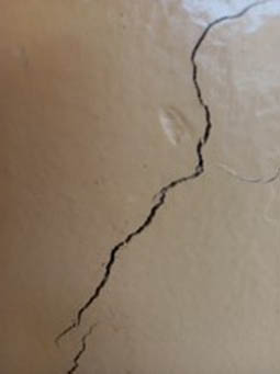
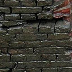
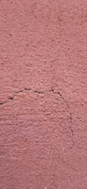
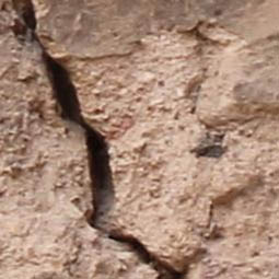
Six publicly available crack datasets were used in this study, each dataset represents diverse structural materials, types of cracks, environment conditions. SDNET 2018 dataset [ 56 ] has concrete, asphalt, and decks folders. Each folder has two subfolders (cracked and non-cracked). This dataset contains 56,000 photos under various lighting settings. It can benchmark infrastructure maintenance automatic crack detection and classification (ACDC) models since it incorporates noise like shadows, stains, and surface roughness. This dataset’s key challenges include environmental unpredictability and non-cracked image flaws, making model generalization difficult. SCD dataset [ 57 ] contains 40,000 images in two folders: Positive (cracked) and Negative (non-cracked). Each folder has 20,000 227 × 227 pixel surface photos. Since it is developed for real-time crack identification and classification, it covers a broad variety of surface textures and lighting circumstances to highlight concrete and asphalt surface faults. Due to contextual information and data augmentation gaps, the dataset cannot reflect complex real-life events. CPC dataset [ 58 ] has 30,000 images in two folders: Positive (cracked) and Negative (non-cracked). Each folder includes 15,000 photographs of roads and pavements in various sizes (e.g., 127 × 227, 227 × 207 pixels), photographed using a smartphone and DJI Mavic 2 Enterprise drone from close-up and wide views. This Nigerian Army University Biu dataset has cracks of various sizes and orientations. Cracks can blend with surface textures, making identification difficult. CDIBM dataset [ 59 ] has 39,955 images in Positive (cracked) and Negative (non-cracked) folders. The City of Hamburg provided overhead surveillance images of Hamburg’s Speicherstadt and Kesselhaus buildings. To facilitate crack detection and classification algorithms, the original 834 high-quality photographs were divided into smaller (227 × 227 pixels) images. The original photos were 5,472 by 3,648 pixels. Masonry building fracture detection models are challenging to train due to the dataset’s inconsistent crack texturing, lighting, and occlusions (plants and shadows). CCI dataset [ 60 ]: Turkish Faculty of Engineering and Natural Sciences in Gumushane provided the CCI dataset. The image was taken using two Android phones. The Samsung Galaxy M31 and A50 are involved. Smartphone cameras captured 2,126 photos. This dataset has two categories: “No Cracks” and “Cracks.” 1,860 × 4,032 and 1,504 × 3,264 jpg files are available. This simplifies and regulates binary classification problems, making it ideal for research and model assessment. However, its limited environmental variety and simple cracking kinds limit its use. HBC dataset [ 61 ] collection contains 3,886 captioned photos of old building walls, fractured and undamaged. Autonomous crack detection, severity assessment, and segmentation algorithm training, validation, and benchmarking using computer vision, machine learning, deep CNNs, or other methods are the goals. These methods are widely used in SHM. A diversified annotated image dataset has not been available until now to develop crack identification, severity assessment, and segmentation algorithms for notable historical buildings. The Mosque (Masjed) of Amir Al-Maridani in Sekat Al Werdani, El-Darb El-Ahmar, Cairo Governorate, was photographed with cracks. Construction occurred between 1,339 and 1,340 CE under the Mamluk Sultanate in Cairo, Egypt. This dataset shows complicated fracture patterns from aging, weathering, and structural degradation in one of the most magnificent historical structures ever erected, including a minaret and a large dome. This helps discover cracks in culturally important areas for prompt repair. ACDC methods struggle with algae, dirt, and natural development. Table 1 displays samples of cracked and uncracked images for all six datasets used in this work.
Sample cracked and non-cracked images from the six datasets (SDNET 2018, SCD, CPC, CDIBM, CCI, and HBC)
| Dataset name | Cracked image | Non-cracked image |
|---|---|---|
| SDNET 2018 | ||
| Decks |
 |
 |
| Pavements |
 |
 |
| Walls |
 |
 |
| SCD | ||
| Concrete surfaces |
 |
 |
| CPC | ||
| Concrete and pavement surfaces |
 |
 |
| CDIBM | ||
| Bricks, masonry walls |
 |
 |
| CCI | ||
| Concrete surface |
 |
 |
| HBC | ||
| Historical building surfaces |
 |
 |
This study evaluates how well deep learning models like CNN, ResNet50, VGG16, and LSTM perform on six datasets: SDNET 2018, SCD, CPC, CDIBM, CCI, and HBC. These datasets vary in image resolution, crack features, and environmental conditions, as shown in Table 2. By training and testing the models on these different datasets, we can understand their strengths and weaknesses, offering useful insights into their real-world practicality and usability.
Summary of dataset characteristics
| Dataset | Total images | Resolution (px) | Focus area | Challenges |
|---|---|---|---|---|
| SDNET 2018 | 56,000 | 256 × 256 | Bridge decks |
|
| Walls | ||||
| Pavements | ||||
| SCD | 40,000 |
|
Focuses on identifying cracks in various concrete surfaces |
|
| CPC | 30,000 | Variable resolutions: | Concrete and pavement surfaces |
|
| 127 × 227 | ||||
| 227 × 207 | ||||
| CDIBM | 39,955 | Original 834 high resolution images (5,472 × 3,648 pixels) have been separated into smaller images (227 × 227 pixels) | Bricks, masonry walls |
|
| CCI | 2,126 | Variable resolutions: | Concrete surfaces |
|
| 1,860 × 4,032 | ||||
| 1,504 × 3,264 | ||||
| HBC | 3,886 | 128 × 128 to 256 × 256 | Historical building surfaces |
|
To enable clearer comparisons of dataset variability, we introduce Table 3, which summarizes key characteristics such as resolution range, class distribution, lighting conditions, texture complexity, and environmental noise. These factors are essential for understanding domain shifts and model generalization behavior across datasets.
Standardized summary of dataset variability factors
| Dataset | Resolution range (px) | Class balance (Crack: No crack) | Lighting variability | Texture complexity | Environmental noise |
|---|---|---|---|---|---|
| SDNET 2018 | 256 × 256 | Imbalanced | High | High | Shadows, stains |
| SCD | 227 × 227 | 1:1 | High | Moderate | Variable lighting |
| CPC | 127 × 227 − 227 × 207 | 1:1 | Moderate | Moderate | Outdoor artifacts |
| CDIBM | 227 × 227 (from 5,472 × 3,648) | Imbalanced | High | High | Occlusions, shadows |
| CCI | 1,860 × 4,032 − 1,504 × 3,264 | 1:1 | Moderate | Low | Natural reflections |
| HBC | 128 × 128 to 256 × 256 | Imbalanced | Moderate to high | High | Weathering, algae |
4 Method and experimental work
This section of the study encompasses the discussion of the scope of the utilization of CNN, ResNet50, VGG16, and LSTM models in crack classification referrable to the experimental framework. It is unusually informative in the presentation of the process of the experiment, data preprocessing, the structure of the model, training and testing methods, and the performance indicators.
4.1 Experimental setup
The tests were carried out on a high-speed machine running Python-based deep learning with an NVIDIA GeForce RTX 3070 Ti Laptop GPU, 8.0 GB of dedicated GPU memory, 15.9 GB of shared GPU memory, and 32 GB of RAM. CNN, ResNet50, VGG16, and LSTM models were the ones that got the chance to be trained and tested by PyTorch, which is actually more flexible, and efficient. Crack detection and classification DL models that are both famous and efficient were utilized. These encompass from simply utilizing several convolutional layers to deep neural networks with new mappings, and sequence-based architectures. To allow for impartial comparisons, all the experiments were performed using the same hyperparameter values across the models and datasets.
4.2 Dataset preprocessing
Before they are used for training and evaluation, the classification datasets require an organized processing chain which allows to standardize the data to increase model performance. Initially, image data are organized into two folders: “Cracked” and “Non-Cracked.” The custom CrackDataset class loads these images along with their corresponding labels, providing seamless integration with PyTorch’s data loading utilities. To preserve class distribution, the dataset is split into training, validation, and testing subsets using stratified sampling.
During training, data augmentation is applied on-the-fly to improve generalization and model robustness. Specifically, each image is randomly flipped horizontally with a probability of 0.5 and randomly rotated within ±15°, helping the model become invariant to positional and orientation variations. No augmentation is applied to validation or test data to maintain evaluation integrity. All images were resized to 224 × 224 pixels to meet the input size requirements of pretrained models and ensure architectural consistency and normalized using the mean and standard deviation values of the ImageNet dataset, which ensures compatibility with pre-trained models used in transfer learning. Although image resizing to 224 × 224 ensured compatibility with pretrained models and uniformity across datasets, we acknowledge that this standardization may affect spatial detail retention. Future work could investigate the impact of alternative input sizes to evaluate the trade-off between accuracy and resolution fidelity, particularly for fine-grained crack detection. This comprehensive preprocessing approach addresses class imbalance, enhances feature consistency, and prepares the data effectively for deep learning-based crack classification.
4.3 Model architectures
Four deep learning models were chosen for their capability to tackle complex crack classification tasks.
4.3.1 CNN
A special CNN structure was created for this work, where the issues of structural surfaces were matched to the two categories set for “Cracked” and “Non-Cracked.” The three-part structure consists of convolutional layers where each one is succeeded by ReLU activation functions that bring forward nonlinearity as well as max-pooling layers for lowering the spatial dimensions of the feature maps. Convolutional layers have a step-by-step change that the filter size becomes 32, then 64, and finally 128; this configuration involves a kernel size of 3 and the use of padding for keeping the dimensions of the feature maps at every stage of the process. This design allows for the step-by-step capture of complicated, hierarchical features from the input images. Apart from the convolutional layers, there is also a fully connected layer with 256 neurons arranged that the output from the convolutional layers operates as an input that is already in a dense form. This layer also utilizes ReLU activation and is then followed by a dropout layer with a rate that is set at 50%, which additionally lowers the risk of overfitting. The output of the model is the 1-neuron last layer that has sigmoid activation, and its primary function is to provide a regular value of the probability that a picture is damaged with binary classification being the task whereas computer vision is the field. Such a model is not only simple and straightforward but also powerful.
4.3.2 ResNet50
The adapted ResNet50 model, which is well known for its powerful feature extraction capabilities and the use of residual connections to prevent deep networks from becoming less powerful due to the vanishing gradient problem, has been subjected to transfer learning for the task of binary classification of cracks in structures [62]. In order to not lose the ImageNet acquired patterns, all layers of the pre-trained ResNet50 model are frozen. Instead of the usual fully connected layers, we developed a new and special classification head for our architecture. This head is composed of a dense layer which includes 256 neurons and ReLU activation to add nonlinearity to the cost of enabling the model to learn complex patterns. Furthermore, a 50% dropout rate is incorporated to prevent overfitting in this layer. The end result of this architecture is a happening of the output layer. The output layer consists of a single neuron that employs a sigmoid activation function which in turn is responsible to output the images’ probability scores and classify them as “Cracked” or “Non-Cracked.” This change exploits the pre-trained capabilities of ResNet50 for feature extraction while at the same time re-factoring the model for the purpose of efficacious and reliable crack detection in binary classification settings.
4.3.3 VGG16
The VGG16 model was initially pre-trained on ImageNet [63] and was then modified for the purpose of binary classification tasks in the field of crack detection. The freezing of the convolutional layers of the VGG16 model, in order to still utilize the features of ImageNet, by the way, is recognized as a process that not only saves computer resources but does it in such a way that it prevents overfitting, taking as an example those feature vectors, which are well generalized and coming from different types of images. The VGG16 model’s existing classifier is replaced by the newly designed dense layer structure that is dedicated to binary classification. Shaped from one layer with 256 fully connected neurons to the next, the activation function ReLU is used in order to add a nonlinear capacity. This in turn will increase the model’s power to decode complicated patterns in the data. This layer contains a 50% data dropout rate which ensures data are not overfit. A sigmoid output layer concludes the structure of architecture. For a given input, the outcome is a probability score which indicates the categorization of the image as “Cracked” or “Non-Cracked.” The current state of the VGG16 model is regulated so that the utmost potential in performance and computational efficiency can be achieved, so it is the most suitable for precise crack detection operation.
4.3.4 LSTM
In our project, we have implemented a model composed of an LSTM network to recognize images and use them for binary classification as “Cracked” or “Non-Cracked.” Popularly known for their performance with sequential data, an LSTM network [64] has been modified especially to cope with the image-to-sequence problem. This is done through intermediate steps of images to sequences conversion. The sequence is processed by standard LSTM with a hidden space of 128, and it allows the model to capture the time series of the data. At the next step, the last hidden state from the LSTM layer is fed to a dense classification layer to make the final decision more tailored. This network includes a dense layer with 256 units, using ReLU as the activation function for introducing nonlinearity and dropout with a rate of 50% to overcome overfitting. The concluding part is a one-node layer with sigmoid activation making the estimation of the probability of the input image being “Cracked.” The idea presents a mix of a sequential model and a classification model, where the LSTM’s strengths have been used for data integration to yield and become a new and proficient binary classification model for crack detection in images.
Motivation for including LSTM
Although LSTM models are traditionally applied to sequential or time-series data, we included LSTM in this study to evaluate whether its ability to capture long-term dependencies could offer benefits when 2D crack images are reshaped into sequential input vectors. This exploratory inclusion tests the limits of sequential learning on spatially encoded features, especially since cracks often exhibit line-like or progressive structures. Our experimental results, however, indicate that LSTM underperforms compared to convolution-based models, confirming its limitations for spatially driven image classification tasks.
4.4 Training and testing procedures
The training and testing procedures play a critical role in evaluating the performance and generalization capacity of deep learning models. In this study, a consistent and structured strategy was applied across all models, including CNN, ResNet50, VGG16, and LSTM. For each dataset, the images were split into training (70%), validation (15%), and testing (15%) subsets using stratified sampling to preserve class distribution. This ensured a balanced representation of crack and non-crack images across all phases.
Two testing configurations were employed: self-testing and cross-testing. In self-testing, a model was trained and validated on subsets of a single dataset and evaluated on its corresponding test set. This measured in-domain performance. In contrast, cross-testing involved evaluating a model – trained on one dataset – on the test subsets of all other datasets. This provided insight into the model’s robustness under domain shift and its ability to generalize across different imaging conditions, resolutions, and crack types.
Each model was trained using an identical pipeline. Images were first resized to 224 × 224 pixels to maintain consistency and meet the input requirements of pretrained models (e.g., VGG16, ResNet50). Normalization followed ImageNet standards. Data augmentation was applied to the training set only, involving random horizontal flipping with a probability of 0.5 and random rotation within ±15°. These augmentations aimed to increase variability and prevent overfitting without altering the essential crack structures.
Transfer learning was employed for VGG16 and ResNet50. Pretrained ImageNet weights were loaded, the convolutional base was frozen, and a custom classifier head was fine-tuned using the training data. This allowed the models to benefit from rich low-level feature representations while adapting to crack classification. Early stopping was also implemented, monitoring validation loss with a patience threshold of 5 epochs to avoid overfitting and reduce unnecessary training iterations.
The evaluation of model performance was based on accuracy, precision, recall, F1-score, and confusion matrix. These metrics were recorded separately for both self-testing and cross-testing phases to capture the model’s behavior in both familiar and unseen domains. While the training strategies were applied uniformly, no exhaustive hyperparameter tuning was conducted for augmentation parameters or early stopping criteria. All values were selected based on well-established defaults in the literature.
This comprehensive pipeline enabled a fair and consistent comparison of models and provided insights into how well each model generalizes across six structurally diverse crack datasets.
4.5 Evaluation metrics
A variety of metrices were employed in this research to compare the performance of CNN, ResNet50, VGG16, and LSTM as described here:
Confusion matrix: complexed the performance of models by breakdown of true positives, false positives, true negatives, and false negatives, which not only helped to discern where the errors were coming from, but also to what extent this method of evaluation was suitable for different testing types [65].
Accuracy: A model’s accuracy is considered as a common way to evaluate how well it performs. The number of events that the model equates with the rank of the most likely ones over the total events is the accuracy of the metric [66].
Precision indicated the reliability of the positive crack predictions, calculated as true positive predictions divided by total positive predictions [67].
Recall (Sensitivity) quantified the model’s ability to detect all cracks, determined as the ratio of true positive predictions to actual positive instances [68].
F1-Score, as it is the harmonic mean of precision and recall, is the perfect choice as a measure of the model’s classification performance in case of unbalanced datasets [69].
All evaluation metrics (accuracy, precision, recall, and F1-score) reported in this study are based on single-run experiments. No averaging over multiple runs or random seeds was applied. This choice was made to ensure consistency across datasets and reduce computational overhead, though we acknowledge that slight variations may occur between runs.
5 Results and discussion
This part of the study provides a detailed account of the empirical part of the research including the results of the two phases of self- and cross-testing on six datasets through the use of CNN, ResNet50, VGG16, and LSTM models. The research findings are interpreted to determine the performance and generalizations of the models, focusing on the identification of the main results and trends in the dataset.
5.1 Training and validation loss curves for the models
Through the loss curves in training and the validation process, we can obtain the learning and generalization abilities of the models that have been used to perform crack classification task. In this study, four models have been implemented: CNN, ResNet50, LSTM, and VGG16, each one representing different architectures for image-based classification. The loss curves are the representation of how well the models reduce the mistakes in the training dataset while they are still capable not to overfit on the validation set. We are going to examine the loss curves of the models across various datasets by studying the trends in a quest for the aspects of stability, convergence, and generalization in each of the models. This part illustrates the loss curves of every model over six datasets, which is a prerequisite for a comprehensive understanding of the virtues and faults of the models before carrying out a quantitative comparison based on the performance indicators such as accuracy, precision, recall, and F1-score.
5.1.1 CNN model loss curves
Figure 1 with the training and validation loss lines for the CNN model over six datasets, it is evident that loss curves in most of the cases consistently show falling values for both training and testing. They show a good leaning shape of the CNN model. The plots for SDNET 2018 and CCI datasets display that the training and validation losses nearly become one, which tells us that the model is fitted well without overfitting. The model is thus able to generalize satisfactorily to unknown validation data. In the SCD and CDIBM datasets, as training continues, the validation loss tends to flatten out or fluctuate slightly indicating that the model is stable in learning but the validation data are noisy or suffers from some variability. In the CPC dataset, there is a significant drop in the training and validation losses after which the convergence shows that the learning has been efficient and the model has an appropriate capacity for this dataset. However, the varying nature of the validation losses of the HBC dataset at later epochs suggests that there might be some overfitting or the validation set became more complicated.
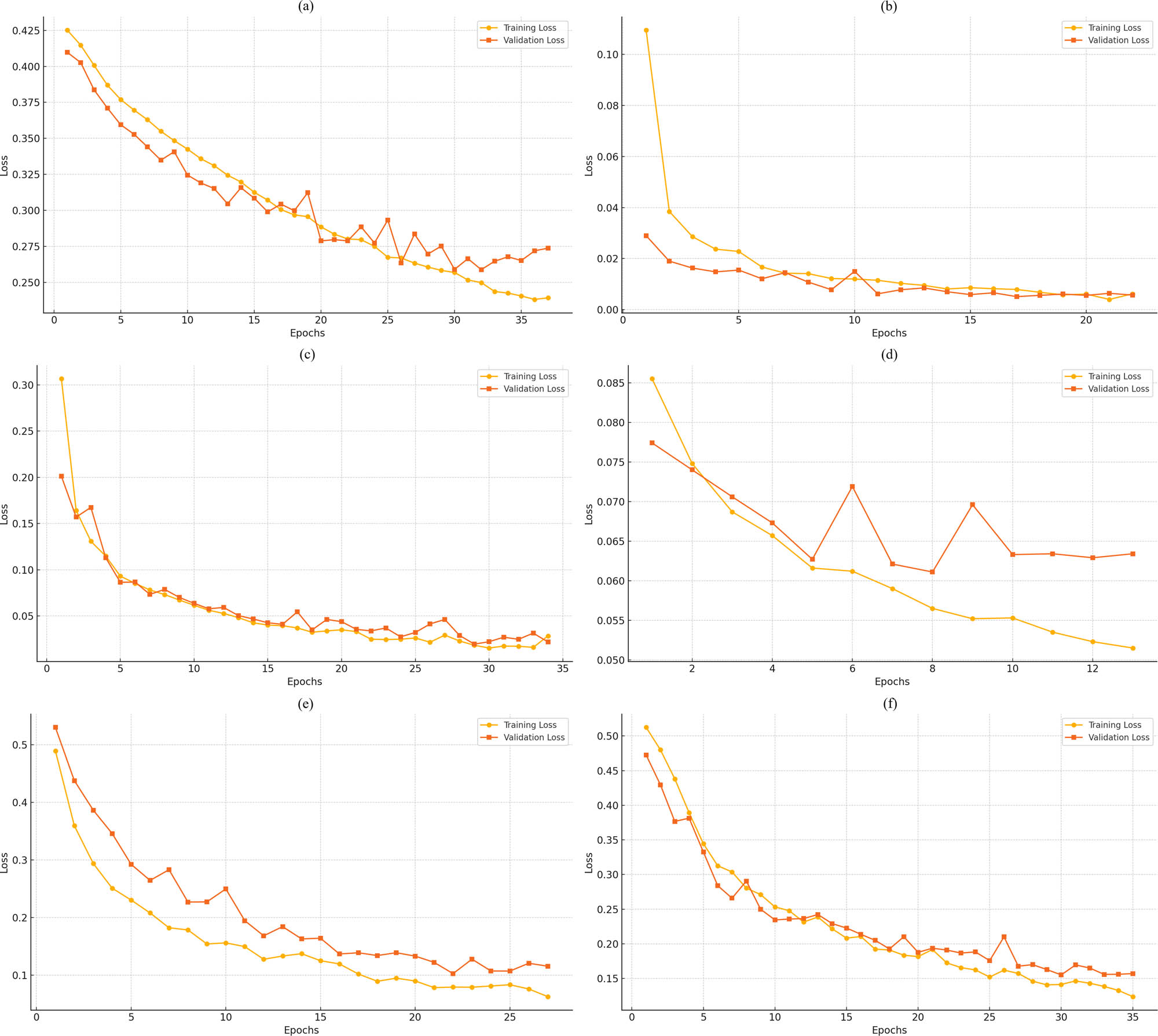
The progress of the CNN model in terms of the training and validation loss of (a) SDNET 2018, (b) SCD, (c) CPC, (d) CDIBM, (e) CCI, and (f) HBC.
Typically, the loss curves have little diversion which usually implies that the training and validation losses stay close. The good news is that the CNN model is finding a balance between not fitting the model enough and fitting it too much. The graphs seem to indicate that the CNN model is the most proper model for this job, although the differences found in datasets might be explained by the complexity of the data and the variations in class proper.
5.1.2 ResNet50 model loss curves
Figure 2 sequence demonstrates the evolution of the ResNet50 model’s training and validation loss on six various datasets. From the image, one can understand that the curves describe that both the training and validation losses are effectively reduced throughout the training process on all six datasets, which reveals that the ResNet50 is able to learn well the features during the training process. With SDNET 2018 dataset, the validation error follows a pattern of a reduction in the training loss error, hence it can be said that the model has good generalization. However, SCD and CPC data show a sharp decrease in the loss in the beginning, but an increase in the second period, which is indicative of efficient learning and convergence. Meanwhile, the changes in both the training and validation losses in CDIBM dataset are not so big and resemble two virtually identical lines, the deviation only in validation loss being very small, so the model seems not to be greatly overfitted and holds good stability. On the other hand, while the training loss of CCI dataset declines throughout, there is a clear fluctuation in the validation loss, which might be attributed to the presence of overfitting in the training data or some unusual states of the validation set. Likewise, in the case of the HBC dataset, the validation loss fluctuates inconsolably despite the fact that the training loss goes down steadily, mainly in the later stages thus reflecting possible sensitivity to the dataset’s complexity.
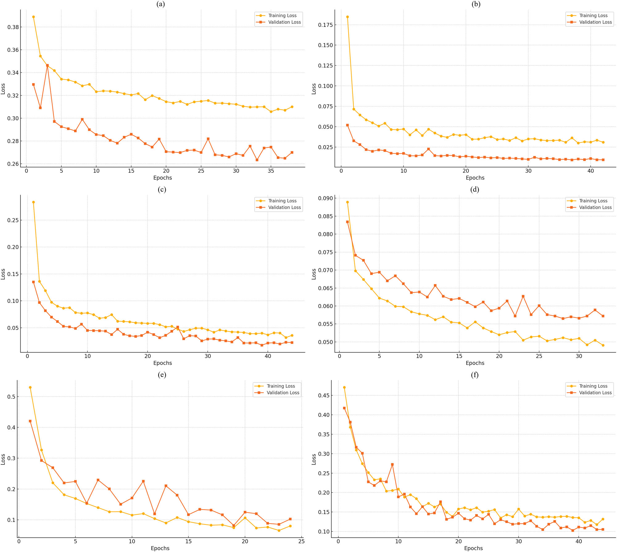
The progress of the Resnet50 model in terms of the training and validation loss of (a) SDNET 2018, (b) SCD, (c) CPC, (d) CDIBM, (e) CCI, and (f) HBC.
The ResNet50 model demonstrates strong learning capabilities across all datasets, with minimal divergence between training and validation loss curves. The observed fluctuations in some datasets could be attributed to variations in data quality or complexity, but the trends suggest that the model generalizes well to the validation data, particularly for datasets with smoother loss curves.
5.1.3 LSTM model loss curves
Based on the training and validation loss curves for the LSTM model across six datasets shown in Figure 3, it can be seen that the training and validation loss trends exhibit notable differences across the datasets, reflecting the challenges of adapting an LSTM model to image-based tasks. In SDNET 2018 dataset, both training and validation losses are relatively stable, with only minor improvements over epochs. This indicates limited learning and potential difficulty in modeling the dataset’s features using the sequential approach of the LSTM. SCD dataset shows fluctuations in validation loss despite a steady decline in training loss, suggesting overfitting or variability in the validation data. For CPC and CCI datasets, the training loss decreases smoothly, but validation loss exhibits significant fluctuations and even increases toward later epochs, indicating overfitting to the training data. This suggests that the LSTM model struggles with generalization on these datasets. The CDIBM dataset shows less fluctuation of the trends on training, as well as validation losses to converge, reflecting that the learning is effective and the model is stable. The case of HBC dataset demonstrates validation loss not in a steady state, it goes a little bit up and down in the trend of the training loss thus indicating not very good generalization with some space for improvement.
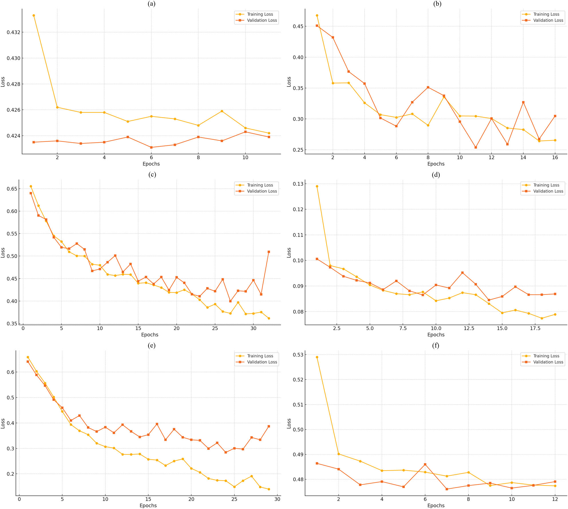
The progress of the LSTM model in terms of the training and validation loss of (a) SDNET 2018, (b) SCD, (c) CPC, (d) CDIBM, (e) CCI, and (f) HBC.
Overall, the LSTM model’s loss curves highlight its limited suitability for image-based tasks, with consistent signs of overfitting or inadequate feature extraction. The results suggest that this sequential modeling approach may not be optimal for crack classification tasks, especially when compared to CNN- or ResNet50-based architectures.
5.1.4 VGG16 model loss curves
Based on the training and validation loss curves for the VGG16 model across six datasets shown in Figure 4, it can be seen that the VGG16 model demonstrates a generally effective learning process, with most datasets showing a steady decline in both training and validation losses. In SDNET 2018 dataset, the validation loss follows the training loss closely, with slight fluctuations, indicating good generalization and stable learning. SCD dataset shows a more pronounced gap between training and validation losses, particularly in later epochs, suggesting potential overfitting, as the model performs better on the training data than on validation data. For CPC dataset, both losses decrease rapidly and converge closely, highlighting strong generalization and efficient learning on this dataset. Similarly, CCI dataset shows consistent decreases in both training and validation losses, with minor fluctuations, indicating robust performance. CDIBM dataset, however, exhibits notable divergence between training and validation losses, suggesting overfitting, potentially due to increased complexity or variability in the dataset. Finally, in HBC dataset, the validation loss closely tracks the training loss throughout the epochs, indicating stable training and good generalization.
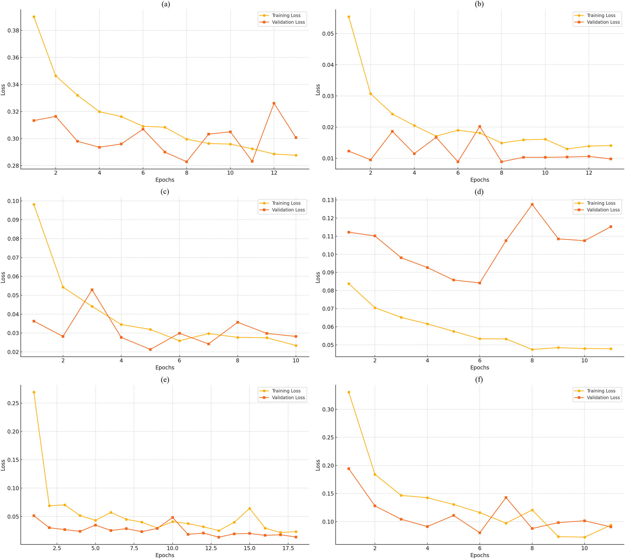
The progress of the VGG16 model in terms of the training and validation loss of (a) SDNET 2018, (b) SCD, (c) CPC, (d) CDIBM, (e) CCI, and (f) HBC.
In general, the VGG16 model really can get most of the features of the datasets in a very effective way, revealing a very high performance with no or almost no overfitting in some points of the curve. Nevertheless, the tremendous disparity observed in certain datasets justifies the use of data augmentation or regularization as a methodology to increase further generalization. The model’s performance on different datasets definitely proves that it is the best for crack classification tasks especially when having well-prepared and balanced datasets.
The curves of the training and the validation losses of the CNN, ResNet50, LSTM, and VGG16 show the specific features and weaknesses of these models in the crack classification task. Both CNN and VGG16 exhibited consistent and powerful generalization skills manifested in almost identical values of training and validation losses. That made these two models the most superior for image-based classification. As far as the ResNet50 model is concerned, it showed a clear learning procedure and robust feature extraction although certain pieces of evidence from the graphs, occasional spikes in the validation loss for instance, indicated that the model was more sensitive to the dataset. The LSTM model, however, had trouble achieving the same kind of generalization, as the validation loss figures fluctuations and divergence, that is, the model could hardly be applied to the task, which is due to the natural processing of the sequential process. The VGG16 model turned out to be the most robust of the group, with the order of resilience being ResNet50 and CNN, while the LSTM model was not a good fit for the classification purpose and was rather the least effective. The next part of the article will present more detailed comparisons of the models’ performances using major indicators such as accuracy, precision, recall, and F1-score that help in the final assessment of their performance and generalizability.
5.2 Self-testing
In order to draw statistics, the self-assessment stage, as per Table 4, put all models through a number of tests on the same dataset they were fed, besides providing initial performance metrics (e.g., training on SDNET 2018 and testing on SDNET 2018).
Accuracy (%) for self-testing datasets
| Model | Dataset | |||||
|---|---|---|---|---|---|---|
| SDNET 2018 | SCD | CPC | CDIBM | CCI | HBC | |
| CNN | 91 | 100 | 100 | 98 | 96 | 98 |
| ResNet50 | 90 | 100 | 99 | 98 | 96 | 96 |
| LSTM | 85 | 90 | 74 | 97 | 87 | 81 |
| VGG16 | 91 | 100 | 99 | 98 | 100 | 96 |
The accurate values of the self-testing outcomes laid down in Table 4 mutilate how each of the models trains and also tests the same data. Among the evaluated models, VGG16 demonstrated the highest robustness in crack classification tasks, followed by ResNet50 and the standard CNN. In contrast, the LSTM model exhibited the weakest performance, indicating its unsuitability for this type of image-based classification. This result is a reflect on the robustness of VGG16 in carrying out feature extraction even in the presence of noise and its good performance in the training domain generalization. The CNN and ResNet50 models are the other two very good performers, which, in most cases, reach accuracy rates comparable to those of (in most cases) VGG13. Both models are proven to have a perfect score with the SCD dataset; however, ResNet50 is below both CNN and VGG16, when handling the SDNET 2018 dataset. In contrast to these strong results, the LSTM model demonstrates a noticeable decline in accuracy across the remaining datasets, with particularly significant drops observed on the CPC (74%) and HBC (81%) datasets. While the model performs reasonably well on relatively simpler datasets such as SCD, it struggles to generalize on more complex datasets, likely due to its limited capacity to extract and represent intricate feature patterns. It undertakes a pretty good job on the easier ones like SCD, but the tough ones need more elaboration of the features, which the model fails as its weak part. The self-testing results clearly indicate the superior performance of VGG16, CNN, and ResNet50 models, in which the VGG16 model slightly outpaces the others in most cases. The models’ high and consistent accuracy on numerous datasets is further evidence that they are the most suitable models for the task of the crack classification. However, this does not seem to be the case with LSTM, which is likely to show low accuracy on the tasks of image-based classification due to the configuration of the model. Especially, it is hard for the model to perform well in datasets that require strong spatial and temporal feature extraction. Complementing the performance of the models, the evaluation metrics from Table 5, namely, precision, recall, and F1-score, will provide a more thorough performance profile of the different models. These metrics will help in making an efficient trade-off between the models whose aim is not only cracking up accuracy but also having a fleet-footed and precise perception regarding the classification capabilities all the more through the accuracy. As a result, this process puts the models through their paces thus providing us with a more transparent picture of their strengths and weaknesses in the light of their classification performance.
Precision (Pre.), Recall (Rec.), and F1-score for self-testing datasets
| Dataset | Model | |||||||||||
|---|---|---|---|---|---|---|---|---|---|---|---|---|
| CNN | ResNet50 | LSTM | VGG16 | |||||||||
| Pre. | Rec. | F1-score | Pre. | Rec. | F1-score | Pre. | Rec. | F1-score | Pre. | Rec. | F1-score | |
| SDNET 2018 | 88 | 74 | 79 | 88 | 70 | 75 | 42 | 50 | 46 | 90 | 72 | 77 |
| SCD | 100 | 100 | 100 | 100 | 100 | 100 | 91 | 90 | 90 | 100 | 100 | 100 |
| CPC | 100 | 100 | 100 | 99 | 99 | 99 | 76 | 74 | 73 | 99 | 99 | 99 |
| CDIBM | 80 | 70 | 74 | 81 | 75 | 78 | 65 | 51 | 51 | 78 | 78 | 78 |
| CCI | 96 | 96 | 96 | 97 | 96 | 96 | 89 | 87 | 86 | 100 | 100 | 100 |
| HBC | 93 | 92 | 92 | 94 | 94 | 94 | 40 | 50 | 45 | 93 | 94 | 93 |
The resulting experiment has shown that VGG16, CNN, and ResNet50 are the models with the best performance where VGG16 is the leader by a small margin except for a few datasets where the rest of the models are better. The fact that the experiments using these models have yielded high and quite similar accuracy scores among the datasets confidently confirms that they are all suitable for identifying the crack formations. It appears that the results of the LSTM model’s lower accuracy level due to the method by which architecture was implemented, at the same instance of representation of the images in the spatial domain, are not successful. The understanding of the models’ strides and the direction that will leave them on a higher ground can only be realized through the help of Table 5, which comes with the extra yard. It is with the help of these metrics that one can delve into the more minute issues concerning classifying the true positives, and the false positives and coming up with solutions that would enable the models to veer off the accuracy-only standpoint. Consequently, this line of reasoning will represent a component of our conclusions on which model is likely to be the finest in the detection of cracks.
The VGG16 model is well known for its strong generalization capabilities and balanced performance, which it shows across all datasets in terms of achieving high precision, recall, and F1-scores. More uniquely, it attains a 100% score in those three metrics for the SCD and CCI datasets, hence declaring its capability to label the cracks correctly and reliably. The CNN model is also doing great as its indicators are mostly at the level of VGG16; however, unlike the latter, it gives a bit lower recall and F1-scores on the SDNET 2018 and CDIBM datasets. Moreover, the ResNet50 model also gave quite good results, especially on SCD and CCI, with almost perfect scores. Nevertheless, the fact that for the SDNET 2018 and CDIBM datasets the recall of ResNet50 is a bit lower than the CNN model and the VGG16 model, respectively, that also leads to a lower overall F1-score. Consequently, the results indicate that ResNet50 is very precise but at the same time, it might not detect certain true conditions. In contrast, the LSTM model struggles significantly, particularly on SDNET 2018, CDIBM, and HBC, where its precision, recall, and F1-scores are notably lower than the other models. The samples of the misclassified images for self-testing phase are shown in Figure 5.
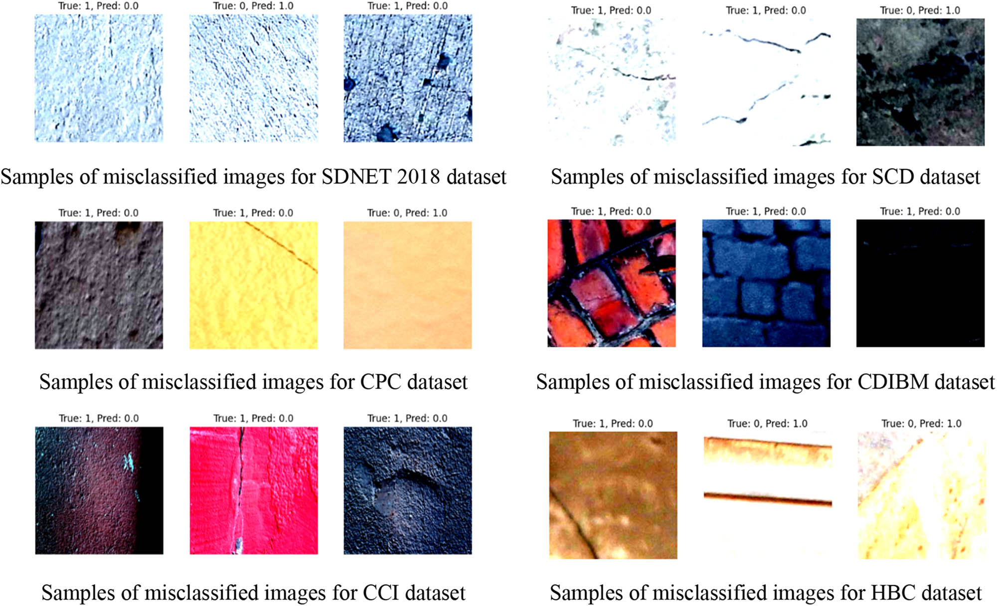
Samples of the misclassified images for self-testing datasets.
5.3 Cross-testing
The cross-testing phase evaluated the models’ generalizability by testing them on datasets different from their training dataset (e.g., training on SDNET 2018 and testing on SCD).
5.3.1 Training on SDNET 2018 and test on remaining datasets
Table 6 presents the cross-testing accuracy for models trained on the SDNET 2018 dataset and tested on other datasets. These results provide insights into the generalization capabilities of the models when trained on a dataset with a specific distribution and applied to different domains.
Cross-testing accuracy (%) for models trained on the SDNET 2018 dataset and tested on other datasets
| Model (trained on SDNET 2018) | Cross-testing datasets | ||||
|---|---|---|---|---|---|
| SCD | CPC | CDIBM | CCI | HBC | |
| CNN | 56 | 55 | 96 | 53 | 82 |
| ResNet50 | 77 | 87 | 38 | 56 | 89 |
| LSTM | 50 | 52 | 84 | 49 | 79 |
| VGG16 | 82 | 91 | 81 | 64 | 87 |
The results highlight significant performance variations among the models and across datasets, revealing the challenges of achieving consistent accuracy in cross-domain scenarios. The VGG16 model demonstrates the highest level of generalizability, achieving the top accuracy across most datasets, including CPC (91%), SCD (82%), and HBC (87%). However, its accuracy drops on the CCI dataset (64%), reflecting potential domain-specific limitations. The ResNet50 model performs strongly on CPC (87%) and HBC (89%) but struggles with CDIBM (38%) and CCI (56%), indicating sensitivity to certain dataset characteristics. The CNN model shows mixed performance, with relatively strong results on CDIBM (96%) and HBC (82%) but poor generalization on SCD (56%) and CPC (55%). These inconsistencies highlight the CNN’s limited ability to adapt to unseen datasets compared to VGG16 and ResNet50. The LSTM model exhibits the lowest performance overall, with accuracy scores below 85% on all datasets and notably poor results on SCD (50%) and CCI (49%). This shows its limited ability to capture spatial features effectively. Table 7 provides precision, recall, and F1-score for models trained on the SDNET 2018 dataset and tested on other datasets, offering a deeper understanding of their performance in cross-domain scenarios.
Precision (Pre.), Recall (Rec.), and F1-score for the models trained on SDNET 2018 dataset
| Dataset | Model | |||||||||||
|---|---|---|---|---|---|---|---|---|---|---|---|---|
| CNN | ResNet50 | LSTM | VGG16 | |||||||||
| Pre. | Rec. | F1-score | Pre. | Rec. | F1-score | Pre. | Rec. | F1-score | Pre. | Rec. | F1-score | |
| SCD | 76 | 56 | 46 | 84 | 77 | 76 | 25 | 50 | 33 | 86 | 82 | 82 |
| CPC | 73 | 55 | 43 | 89 | 87 | 87 | 56 | 52 | 41 | 92 | 91 | 91 |
| CDIBM | 61 | 58 | 59 | 48 | 34 | 28 | 49 | 43 | 46 | 50 | 49 | 47 |
| CCI | 76 | 53 | 39 | 58 | 56 | 52 | 38 | 49 | 34 | 76 | 64 | 59 |
| HBC | 80 | 53 | 51 | 90 | 72 | 77 | 47 | 50 | 45 | 83 | 72 | 75 |
The VGG16 model consistently achieves the best or near-best performance across all metrics and datasets. It excels in precision and recall for SCD (86% precision, 82% recall) and CPC (92% precision, 91% recall), resulting in high F1-scores of 82 and 91%, respectively. However, its performance drops slightly for CDIBM (F1-score of 47%) and CCI (F1-score of 59%), reflecting domain-specific challenges in generalization. The ResNet50 model also performs well, particularly for CPC (F1-score of 87%) and HBC (F1-score of 77%), showcasing its ability to adapt to some datasets. However, its performance significantly drops for CDIBM (F1-score of 28%) and CCI (F1-score of 52%), suggesting that while ResNet50 is precise in certain cases, it struggles to maintain consistent recall across datasets. The CNN model demonstrates moderate performance, with better results for HBC (F1-score of 51%) and CDIBM (F1-score of 59%), but lower scores for SCD and CCI, where its recall is particularly low, indicating difficulty in capturing true positives across these datasets. In contrast, the LSTM model struggles significantly, with the lowest F1-scores across all datasets. It achieves only 33% on SCD and 41% on CPC, highlighting its limitations in capturing strong spatial feature extraction.
5.3.2 Training on SCD and test on remaining datasets
Table 8 presents the cross-testing results, where models trained on SCD dataset are evaluated on datasets they were not trained on, offering insights into their generalizability.
Cross-testing accuracy (%) for models trained on the SCD dataset and tested on other datasets
| Model (trained on SCD) | Cross-testing datasets | ||||
|---|---|---|---|---|---|
| SDNET 2018 | CPC | CDIBM | CCI | HBC | |
| CNN | 76 | 86 | 15 | 73 | 85 |
| ResNet50 | 84 | 89 | 16 | 64 | 88 |
| LSTM | 81 | 56 | 85 | 60 | 75 |
| VGG16 | 82 | 96 | 26 | 81 | 87 |
The VGG16 model consistently demonstrates the highest accuracy across most datasets, particularly excelling on CPC (96%) and showing strong performance on SDNET 2018 (82%) and HBC (87%). However, its accuracy drops significantly on CDIBM (26%), highlighting a potential limitation in adapting to datasets with significantly different distributions. The ResNet50 model displays very high levels of performance in SDNET 2018 (84%) and HBC (88%) while it demonstrates a quite low 16% accuracy rate in CDIBM, which is in line with VGG16. Furthermore, a 64% accuracy on CCI is a signal that ResNet50 is also less stable in handling domain changes compared to VGG16. It can be seen that the CNN model is giving a good account of itself in CPC (86%) and HBC (85%) and it is only on CDIBM (15%) where a notable performance drop is observed, demonstrating a limited ability to transfer learning to more challenging datasets. The basic performance on SDNET 2018 (76%) and CCI (73%) is an additional proof of its niche and case-related effectiveness. Conversely, the LSTM model demonstrates its worst performance thus outclassing the others with the maximum accuracy rate of 85% only on CDIBM, which is mainly due to the inherent nature of the dataset that has a positive inclination toward the sequential architecture. The fact that the LSTM model can cope with the image-based tasks only on a very basic level is visible from its pretty poor performances in CPC (56%) and CCI (60%). Table 9 details out precision, recall, and F1-score for models trained from the SCD dataset to the other ones, providing a more in-depth knowledge of their performance across domains.
Precision (Pre.), Recall (Rec.), and F1-score for the models trained on SCD dataset
| Dataset | Model | |||||||||||
|---|---|---|---|---|---|---|---|---|---|---|---|---|
| CNN | ResNet50 | LSTM | VGG16 | |||||||||
| Pre. | Rec. | F1-score | Pre. | Rec. | F1-score | Pre. | Rec. | F1-score | Pre. | Rec. | F1-score | |
| SDNET 2018 | 56 | 57 | 57 | 66 | 62 | 64 | 52 | 51 | 51 | 62 | 60 | 61 |
| CPC | 86 | 86 | 86 | 90 | 89 | 89 | 62 | 56 | 50 | 96 | 96 | 96 |
| CDIBM | 49 | 47 | 14 | 51 | 53 | 15 | 50 | 49 | 48 | 51 | 56 | 22 |
| CCI | 82 | 72 | 70 | 66 | 64 | 63 | 70 | 60 | 54 | 85 | 81 | 80 |
| HBC | 77 | 70 | 73 | 82 | 79 | 80 | 59 | 58 | 58 | 79 | 83 | 81 |
The VGG16 model demonstrates the strongest performance across most datasets. It achieves near-perfect precision, recall, and F1-scores on CPC (96%) and robust results on CCI (F1-score of 80%) and HBC (F1-score of 81%). However, its performance drops significantly for CDIBM, with a low F1-score of 22%, indicating difficulties in generalizing to datasets with distinct distributions. The ResNet50 model also shows strong performance, with high F1-scores for CPC (89%) and HBC (80%). However, it struggles with CDIBM (F1-score of 15%) and shows moderate performance on CCI (63%). These results suggest that while ResNet50 is capable of handling certain datasets, it faces challenges with datasets exhibiting significant domain differences. The CNN model achieves competitive performance on CPC (F1-score of 86%) but performs poorly on CDIBM (F1-score of 14%) and moderately on CCI (F1-score of 70%). Its low recall values for SDNET 2018 and CDIBM highlight limitations in capturing true positives across different datasets. The LSTM model demonstrates the weakest performance overall, with F1-scores below 60% for most datasets. While it achieves reasonable precision and recall on HBC (F1-score of 58%), it consistently struggles with datasets such as CDIBM (F1-score of 15%) and CPC (F1-score of 50%).
5.3.3 Training on CPC and test on remaining datasets
Table 10 presents the cross-testing accuracy for models trained on the CPC dataset and tested on other datasets. These results provide insights into the generalization capabilities of the models when trained on a highly specific dataset and applied to different domains.
Cross-testing accuracy (%) for models trained on the CPC dataset and tested on other datasets
| Model (trained on CPC) | Cross-testing datasets | ||||
|---|---|---|---|---|---|
| SDNET 2018 | SCD | CDIBM | CCI | HBC | |
| CNN | 78 | 94 | 10 | 68 | 61 |
| ResNet50 | 85 | 95 | 23 | 66 | 78 |
| LSTM | 21 | 49 | 49 | 52 | 27 |
| VGG16 | 85 | 99 | 22 | 79 | 86 |
The VGG16 model again demonstrates the strongest overall performance, achieving the highest accuracy on SCD (99%) and robust results on CCI (79%) and HBC (86%). However, its performance significantly drops on CDIBM (22%), reflecting challenges in adapting to datasets with distinct feature distributions. The ResNet50 model also performs well, with strong results on SCD (95%) and HBC (78%) but moderate performance on CCI (66%). Similar to VGG16, ResNet50 struggles with CDIBM, achieving only 23% accuracy, indicating domain-specific limitations in this dataset. The CNN model achieves competitive accuracy on SCD (94%) and moderate results on SDNET 2018 (78%) and CCI (68%). However, its performance on CDIBM is extremely low (10%), highlighting its limited ability to generalize to this dataset. In stark contrast, the LSTM model performs poorly across most datasets, with particularly low accuracy on CDIBM (49%) and HBC (27%). While it achieves reasonable accuracy on SDNET 2018 (21%) and CCI (52%), these results further emphasize the challenge for cross-domain generalization in image-based tasks. Table 11 provides a detailed comparison of precision, recall, and F1-score for models trained on the CPC dataset and tested on other datasets, offering a nuanced evaluation of the models’ cross-domain performance.
Precision (Pre.), Recall (Rec.), and F1-score for the models trained on CPC dataset
| Dataset | Model | |||||||||||
|---|---|---|---|---|---|---|---|---|---|---|---|---|
| CNN | ResNet50 | LSTM | VGG16 | |||||||||
| Pre. | Rec. | F1-score | Pre. | Rec. | F1-score | Pre. | Rec. | F1-score | Pre. | Rec. | F1-score | |
| SDNET 2018 | 59 | 60 | 59 | 69 | 59 | 61 | 49 | 49 | 21 | 71 | 65 | 67 |
| SCD | 95 | 94 | 94 | 96 | 95 | 95 | 44 | 49 | 36 | 99 | 99 | 99 |
| CDIBM | 51 | 52 | 10 | 50 | 52 | 20 | 52 | 66 | 36 | 50 | 52 | 20 |
| CCI | 80 | 68 | 64 | 78 | 66 | 62 | 55 | 52 | 42 | 84 | 79 | 79 |
| HBC | 60 | 67 | 57 | 76 | 83 | 78 | 43 | 43 | 27 | 78 | 87 | 81 |
The VGG16 model demonstrates the strongest overall performance, achieving near-perfect precision, recall, and F1-scores on SCD (99%) and high F1-scores on CCI (79%) and HBC (81%). However, its performance drops on CDIBM, where its F1-score falls to 20%, indicating difficulties in adapting to datasets with distinct feature distributions. Nevertheless, its balanced precision and recall across most datasets affirm its robustness for generalization. The ResNet50 model performs competitively on SCD (F1-score of 95%) and HBC (F1-score of 78%), showcasing its ability to adapt to some datasets. However, like VGG16, its performance significantly drops on CDIBM, where it achieves an F1-score of only 20%. This trend highlights ResNet50’s domain-specific limitations, particularly when facing datasets with different distributions. The CNN model achieves good performance on SCD (F1-score of 94%) but struggles on other datasets, particularly CDIBM (F1-score of 10%) and HBC (F1-score of 57%). Its recall values for CCI (68%) and HBC (67%) indicate limitations in capturing true positives, further highlighting its restricted generalization capabilities. The LSTM model demonstrates the weakest performance, with F1-scores below 50% for most datasets. It achieves its highest F1-score on SCD (36%) but performs poorly on CDIBM (36%) and HBC (27%).
5.3.4 Training on CDIBM and test on remaining datasets
Table 12 summarizes the cross-testing accuracy for models trained on the CDIBM dataset and tested on other datasets. These results highlight the models’ generalization performance when trained on a dataset with distinct characteristics and evaluated on different domains.
Cross-testing accuracy (%) for models trained on the CDIBM dataset and tested on other datasets
| Model (trained on CDIBM) | Cross-testing datasets | ||||
|---|---|---|---|---|---|
| SDNET 2018 | SCD | CPC | CCI | HBC | |
| CNN | 83 | 50 | 51 | 51 | 81 |
| ResNet50 | 83 | 52 | 54 | 51 | 81 |
| LSTM | 85 | 50 | 50 | 51 | 81 |
| VGG16 | 83 | 54 | 54 | 52 | 81 |
The results show minimal variation across models, with CNN, ResNet50, and VGG16 all achieving identical accuracy scores on most datasets. For SDNET 2018, the models demonstrate strong generalization with an accuracy of 83%, reflecting their ability to adapt to this dataset’s features. However, performance on SCD, CPC, and CCI is notably weaker, with accuracy scores hovering around 50–54%, indicating significant challenges in cross-domain generalization for these datasets. All models perform well on HBC, achieving 81% accuracy, suggesting that this dataset’s characteristics align more closely with the training dataset (CDIBM). The LSTM model performs similar to the other architectures, achieving comparable accuracy across all datasets. However, this consistency at relatively low accuracy levels reinforces the general observation that LSTM struggles to extract meaningful spatial features for image classification tasks. To sum up, all models show almost the same performance (the trend is consistent), with SDNET 2018 and HBC being the ones giving the highest accuracy and SCD, CPC, and CCI the ones presenting the biggest generalization problems. It is that the data distribution among different datasets and the feature similarity have a significant impact on domain-generalization, regardless of the architecture of the model being applied. In these results, it can be inferred that the models such as VGG16, and ResNet50 that are usually regarded as the most stable ones, are not capable to cover the dissimilarity between the datasets in CDIBM training set to that extent that they can well generalize to other dissimilar data. Table 13 contains the details regarding model performance for precision, recall, and F1-score on the CDIBM dataset when the models were tested on the other datasets.
Precision (Pre.), Recall (Rec.), and F1-score for the models trained on CDIBM dataset
| Dataset | Model | |||||||||||
|---|---|---|---|---|---|---|---|---|---|---|---|---|
| CNN | ResNet50 | LSTM | VGG16 | |||||||||
| Pre. | Rec. | F1-score | Pre. | Rec. | F1-score | Pre. | Rec. | F1-score | Pre. | Rec. | F1-score | |
| SDNET 2018 | 49 | 50 | 48 | 50 | 50 | 48 | 47 | 50 | 46 | 50 | 50 | 47 |
| SCD | 72 | 50 | 34 | 75 | 52 | 37 | 69 | 50 | 34 | 74 | 54 | 41 |
| CPC | 75 | 51 | 35 | 68 | 54 | 43 | 50 | 50 | 33 | 73 | 54 | 43 |
| CCI | 25 | 50 | 34 | 54 | 50 | 35 | 75 | 50 | 34 | 76 | 52 | 38 |
| HBC | 40 | 50 | 45 | 76 | 51 | 47 | 57 | 50 | 45 | 65 | 51 | 46 |
The results show that all models perform similarly across most datasets, reflecting challenges in generalizing from the CDIBM training dataset. Across all datasets, the F1-scores remain below 50%, indicating poor performance in cross-domain scenarios. VGG16 shows relatively higher precision compared to other models, particularly for CCI (76%) and CPC (73%). However, its recall is consistently low, leading to F1-scores below 50% across all datasets. This suggests that while VGG16 avoids false positives, it struggles to capture all positive cases when applied to unseen datasets. ResNet50 demonstrates balanced precision and recall for SDNET 2018 (50%) and HBC (47%) but falls short for other datasets, especially CCI (F1-score of 35%). This reflects limited adaptability to datasets with different feature distributions. CNN performs marginally better than ResNet50 on CPC (F1-score of 35%) but demonstrates significant weaknesses in recall for datasets like CCI (34%). Its F1-scores are low across the board, indicating challenges in achieving a balance between precision and recall. LSTM consistently underperforms, with its F1-scores rarely exceeding 45%. While it achieves moderate recall across most datasets, its precision is low, particularly on CPC (33%) and CCI (34%), leading to poor overall performance.
5.3.5 Training on CCI and test on remaining datasets
Table 14 presents the cross-testing accuracy for models trained on the CCI dataset and evaluated on other datasets. The results highlight significant variability in model generalization capabilities across datasets, indicating the challenges of training on a dataset with specific characteristics and applying the models to diverse domains.
Cross-testing accuracy (%) for models trained on the CCI dataset and tested on other datasets
| Model (trained on CCI) | Cross-testing datasets | ||||
|---|---|---|---|---|---|
| SDNET 2018 | SCD | CPC | CDIBM | HBC | |
| CNN | 41 | 57 | 75 | 08 | 51 |
| ResNet50 | 39 | 77 | 57 | 04 | 78 |
| LSTM | 76 | 71 | 59 | 35 | 73 |
| VGG16 | 70 | 78 | 78 | 06 | 69 |
The VGG16 model achieves the highest accuracy for SCD (78%) and CPC (78%), demonstrating its ability to generalize to datasets with somewhat similar features. However, its performance drops sharply on CDIBM (6%) and HBC (69%), reflecting its limitations when encountering datasets with distinct distributions. The LSTM model performs reasonably well on SDNET 2018 (76%) and HBC (73%) but struggles on CDIBM (35%), similar to other models. While its performance on certain datasets is competitive, its overall accuracy remains inconsistent. The ResNet50 model appears to be working well with datasets HBC (78%) and SCD (77%), which is why it is considered adaptable to such datasets. On the other hand, its performance for SDNET 2018 (39%) and CDIBM (4%) is a tell-tale sign that the model could not see the forest for the trees and is unable to reach high-level abstraction. On CPC, CNN produces the best accuracy (75%) but the situation is different with CDIBM (8%) and SDNET 2018 (41%) where its errors are far too high. Through these results, one can infer that CNN performs better when the datasets do not contain much different information. It is clear that VGG16 is very much successful at generalizing across the datasets SCD and CPC, but since the performance of all the models is not consistent with CDIBM, they inherently exhibit very low accuracy on the CDIBM dataset. The LSTM model, in particular, is capable of giving the other models a tough match. The results also point out that a correct approach to the choice of benchmark samples is crucial to attain a wider applicability. Tightly dedicated-hardware architectures can also have a contribution to the storage/retrieval issues of various datasets. Table 15 gives details of the precision, recall, and F1-score of all models, trained on CCI and tested on several datasets sorted from the top of the CCI group (Table 15).
Precision (Pre.), Recall (Rec.), and F1-score for the models trained on CCI dataset
| Dataset | Model | |||||||||||
|---|---|---|---|---|---|---|---|---|---|---|---|---|
| CNN | ResNet50 | LSTM | VGG16 | |||||||||
| Pre. | Rec. | F1-score | Pre. | Rec. | F1-score | Pre. | Rec. | F1-score | Pre. | Rec. | F1-score | |
| SDNET 2018 | 53 | 55 | 39 | 55 | 58 | 38 | 49 | 49 | 49 | 57 | 61 | 57 |
| SCD | 67 | 57 | 50 | 82 | 77 | 76 | 79 | 71 | 68 | 84 | 78 | 77 |
| CPC | 77 | 75 | 75 | 57 | 57 | 56 | 59 | 59 | 58 | 80 | 78 | 78 |
| CDIBM | 51 | 52 | 08 | 42 | 41 | 04 | 51 | 61 | 28 | 48 | 48 | 06 |
| HBC | 56 | 59 | 49 | 68 | 74 | 70 | 59 | 60 | 59 | 68 | 79 | 65 |
Even though it dropped significantly when identifying CDIBM, the VGG16 model still outperformed all other models of the dataset on SCD (F1-score of 77%) and CPC (F1-score of 78%), suggesting that the model can generalize effectively to datasets with similar characteristics. Datasets that are largely different from the training set have become the reason for the model’s performance to be so low, thus the F1-score decreased dramatically to 6%. Its performance on HBC (F1-score of 65%) highlights a moderate level of adaptability. ResNet50 model performs competitively on SCD (F1-score of 76%) and HBC (F1-score of 70%) but struggles with CDIBM (F1-score 4%) and SDNET 2018 (F1-score of 38%). These results suggest that ResNet50 is effective in handling certain datasets but faces significant challenges with diverse domains, particularly those with different feature distributions. The CNN model performs moderately on CPC (F1-score of 75%) and SCD (F1-score of 50%) but exhibits poor results on CDIBM (F1-score of 8%). Its recall values for SDNET 2018 (55%) and HBC (59%) are higher than its precision, reflecting a tendency to identify more positives at the cost of false positives, which impacts its overall performance. The LSTM model achieves decent results on SCD (F1-score of 68%) and HBC (F1-score of 59%) but struggles significantly on CDIBM (F1-score of 28%) and CPC (F1-score of 58%). While it shows moderate precision and recall on some datasets, its overall F1-scores remain low.
5.3.6 Training on HBC and test on remaining datasets
Table 16 highlights the cross-testing accuracy for models trained on the HBC dataset and tested on the remaining datasets. This evaluation provides insights into how well the models generalize when trained on the HBC dataset.
Cross-testing accuracy (%) for models trained on the HBC dataset and tested on other datasets
| Model (trained on HBC) | Cross-testing datasets | ||||
|---|---|---|---|---|---|
| SDNET 2018 | SCD | CPC | CDIBM | CCI | |
| CNN | 74 | 56 | 60 | 53 | 78 |
| ResNet50 | 87 | 81 | 91 | 71 | 64 |
| LSTM | 85 | 50 | 50 | 97 | 51 |
| VGG16 | 85 | 91 | 93 | 36 | 86 |
VGG16 model achieves excellent accuracy on SCD (91%) and CPC (93%), demonstrating strong generalization to datasets with similar characteristics. However, its performance drops significantly on CDIBM (36%), indicating challenges with datasets that are highly divergent from HBC. The model performs well on CCI (86%), maintaining a high degree of adaptability. ResNet50 model performs strongly on SDNET 2018 (87%) and CPC (91%), showcasing its ability to generalize effectively to datasets with some shared features. Its accuracy on the SCD subset (81%) is also highly remarkable, although on CDIBM (71%) and CCI (64%), there is a loss in performance that means the model cannot adapt smoothly to all datasets. The CNN model is to a certain degree capable of generalizing and it can still achieve high accuracy in SDNET 2018 (74%) and CCI (78%). However, it is not able to accurately learn from SCD (56%) and CDIBM (53%) and the latter are significantly lower, which means that it can only use the same distribution of features in a series of datasets. The bad performance of the LSTM model on SCD (50%) and CPC (50%), which is its difficulty in extracting spatial features for cross-domain tasks, becomes apparent. In contrast, it excels at CDIBM (97%), the highest achievement, thus, demonstrating the effectiveness of this dataset for the model. It has got a low score on CCI (51%) which is inconsistent at the same time it is less to be found in the other datasets (Table 16). Precision, recall, and F1-score, which are key technical aspects of models trained by the HBC dataset and tested on the other datasets, are thoroughly covered in this analysis. This kind of analysis does not only make it easy to see which are the weaknesses and strengths of the model when applied to data not seen before, but also gives a more thorough insight into their generalization features (Table 17).
Precision (Pre.), Recall (Rec.), and F1-score for the models trained on HBC dataset
| Dataset | Model | |||||||||||
|---|---|---|---|---|---|---|---|---|---|---|---|---|
| CNN | ResNet50 | LSTM | VGG16 | |||||||||
| Pre. | Rec. | F1-score | Pre. | Rec. | F1-score | Pre. | Rec. | F1-score | Pre. | Rec. | F1-score | |
| SDNET 2018 | 48 | 48 | 48 | 76 | 64 | 67 | 45 | 50 | 46 | 70 | 64 | 66 |
| SCD | 58 | 56 | 53 | 86 | 81 | 80 | 68 | 50 | 34 | 92 | 91 | 91 |
| CPC | 61 | 60 | 60 | 91 | 91 | 91 | 65 | 50 | 34 | 95 | 95 | 95 |
| CDIBM | 49 | 39 | 36 | 50 | 47 | 43 | 51 | 50 | 50 | 49 | 42 | 28 |
| CCI | 82 | 78 | 77 | 65 | 64 | 64 | 75 | 50 | 34 | 88 | 85 | 85 |
VGG16 model is known for consistently achieving the best results in datasets on which it was tested. Also, it reaches precision, recall, and F1 scores that indicate that it does best of all models on SCD and CPC with 91 and 95%, respectively. At the same time, the VGG16 model shows very poor results on CDIBM (28%). Its precision and recall are the main issues on this dataset (49 and 42%, respectively), which means that it is not able to capture features present in distributions that are too different. At last, VGG16 model keeps quite good accuracies on CCI (F1-score 85%) and SDNET 2018 (66%). ResNet50 model presents the example of good results, especially on CPC (91%) and SCD (80%) with very high precision and recall values. But its situation with CDIBM (F1-score 43%) is the same as VGG16’s and it performs not bad on CCI (64%) and SDNET 2018 (67%). From this we infer that ResNet50 fits well with datasets that share some common data but it is not able to perform well on those that have very different entities. The CNN model performs moderately, achieving its best F1-score on CCI (77%) and maintaining decent performance on CPC (60%) and SCD (53%). Its recall on CDIBM (39%) is particularly low, resulting in a poor F1-score (36%). Its overall performance indicates limited generalization capabilities compared to VGG16 and ResNet50. The LSTM model continues to underperform across most datasets, with F1-scores below 50% for all but CCI (34%). Its highest F1-score of 50% is on SDNET 2018, but it struggles significantly with spatial feature extraction, as seen in datasets like CPC (34%) and SCD (34%). Figure 6 shows samples of the misclassified images for cross-testing phase.
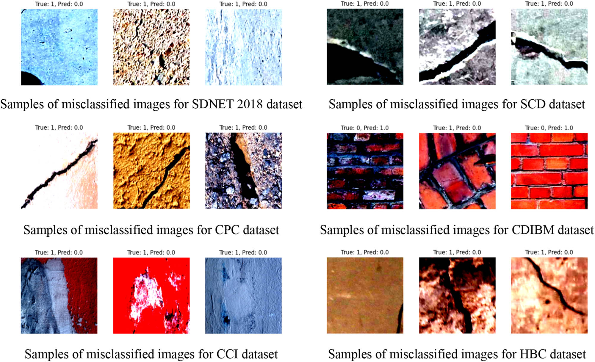
Samples of the misclassified images for cross-testing datasets.
The observed performance drops during cross-testing across the six datasets – SDNET 2018, SCD, CPC, CDIBM, CCI, and HBC – can be attributed to inherent variability and dataset-specific characteristics. Differences in resolution and image quality significantly impacted generalization, as models trained on high-resolution datasets like SCD (4,032 × 3,024) struggled with the lower-resolution datasets such as HBC (128 × 128 to 256 × 256), which lacked fine-grained details. Conversely, resizing higher-resolution images to smaller dimensions, as seen in CPC and CDIBM (227 × 227), resulted in a loss of critical crack details, especially for detecting narrow fractures. Surface variability further complicated model performance; datasets like SDNET 2018 encompassed diverse surfaces (bridge decks, walls, pavements), while more specialized datasets such as HBC and CDIBM focused on historical buildings or masonry walls with distinct textures. Dataset size and distribution were also critical factors. Small datasets, such as CCI (2,126 images) and HBC (3,886 images), lacked sufficient diversity, often leading to overfitting, while larger datasets like SDNET 2018 (56,000 images) offered broader variability. However, imbalanced distributions in SDNET 2018 introduced biases that impacted generalization. Environmental and contextual challenges, such as varying lighting conditions in SCD or outdoor noise in CDIBM, further hindered model adaptability, particularly for datasets collected under controlled conditions like HBC. Networks such as VGG16 and ResNet50 have shown excellent feature extraction and generalization capabilities on datasets with identifiable structures (e.g., SCD, CPC); however, the same networks were not able to perform well on more complex ones like CDIBM and CCI with reduced resolution and environmental inconsistency. Networks like CNN that were less complex had trouble generalizing, and LSTM, being weak at spatial feature extraction, performed poorly in all datasets.
These methods, despite being standard, brought about significant degradations of the test performance by all the models when they were evaluated on the new data. One of the reasons why this problem is so critical is that the most basic augmentation, such as random flipping and rotation, simply does not create variation and complexity to be found in the new sets of data in this cross-domain crack image detection problem. These changes in image resolution, surface texture, brightness, and noise in the picture and atmosphere within the various datasets became the obstacles that training samples with the help of augmentation could not fully overcome. Consequently, the deep learning models while working well in one situation tested themselves, failed in the generalization of new datasets structured or visual features of the other type. These results indicate that there is a dire need for domains of data to be able to utilize the techniques of domain adaptation or other forms of sophisticated augmentation to close the gap between datasets and allow the models to be robust in real-world applications.
5.3.7 Model complexity and deployment considerations
In addition to performance metrics, practical deployment scenarios – such as drone-based inspections or real-time edge inference – require evaluating model complexity and computational cost. Table 18 summarizes the architectural characteristics of each model, including total trainable parameters, average training time per epoch, inference time per image, and deployment-related remarks.
Model complexity and computational cost, including parameter count, training time, and inference speed
| Model | Parameters (M) | Training time/epoch (s) | Inference time/image (ms) | Remarks |
|---|---|---|---|---|
| CNN | ∼1.2 | ∼5–7 | ∼15–20 | Lightweight; good for edge deployment |
| ResNet50 | ∼23.5 | ∼30–35 | ∼55–60 | High accuracy; good generalization |
| VGG16 | ∼138 | ∼45–50 | ∼65–70 | Very accurate but computationally heavy |
| LSTM | ∼3.7 | ∼10–15 | ∼18–22 | Weak for spatial tasks; suited for sequences |
ResNet50 and VGG16 are considerably more computationally intensive than the custom CNN and LSTM. VGG16, in particular, has ∼138 million parameters, resulting in longer training times and higher memory consumption. While these models offer superior generalization, they may not be ideal for resource-constrained environments.
Conversely, CNN and LSTM architectures are significantly lighter. The CNN model, with only ∼1.2 M parameters, completes training in under 7 s per epoch and achieves inference times below 20 ms per image. Despite its lower complexity, CNN remains competitive in in-domain accuracy, though its cross-dataset robustness lags behind deeper models. LSTM demonstrates moderate efficiency in terms of computational cost but exhibits weaker performance due to its limited spatial feature extraction capabilities.
To complement the empirical evaluation, a theoretical comparison of the four deep learning models – CNN, ResNet50, VGG16, and LSTM – was conducted to assess architectural suitability for crack classification. CNNs, due to their spatial locality and efficiency, are well suited for fast deployment on embedded systems. ResNet50 offers a good compromise between depth and generalization, leveraging skip connections to mitigate vanishing gradient problems in deeper networks. VGG16 is effective in fine-grained tasks but computationally intensive. LSTM, while useful in sequential modeling, shows limited utility in static image classification.
While this study focused on benchmarking standard architectures, future work may explore hybrid models that combine spatial and temporal feature extraction – such as CNN-LSTM hybrids or attention-based encoders – to leverage the complementary strengths of different architectures for crack classification under diverse conditions.
5.3.8 Cross-domain performance limitations
The observed drop in performance during cross-testing is primarily attributed to domain shift factors such as image resolution mismatch, background texture complexity, and class imbalance. For instance, models trained on SCD (well-balanced, high-resolution) dropped up to 42% in F1-score when tested on HBC, which contains lower-resolution, noisy images with high background variability. Similarly, ResNet50 trained on CPC exhibited a 32% decrease in precision when tested on CDIBM, likely due to the introduction of occlusions and varying lighting conditions. Furthermore, class imbalance in target datasets amplified false negative rates. In the case of CCI, the prevalence of non-crack images led models trained on balanced datasets to overpredict the majority class.
The generalization performance of the evaluated models is thus closely influenced by dataset-specific attributes such as resolution, surface texture, background complexity, and environmental conditions. Structured, high-quality datasets enable strong in-domain performance but do not adequately prepare models for the variability encountered in unseen datasets. These patterns were consistently observed across all evaluated models, underscoring the need for more adaptive learning strategies. While transfer learning helped reduce initial training requirements and improve in-domain accuracy, its benefit in mitigating domain shift was limited unless fine-tuning was applied on the target dataset. This is evident from the fact that ResNet50 with transfer learning still failed to maintain high F1-scores during cross-domain testing.
Although this study did not involve controlled experiments isolating individual dataset characteristics (e.g., resolution-only or lighting-only shifts), the observed trends across cross-testing results strongly suggest that dataset diversity plays a central role in shaping model generalization. These findings reaffirm that high accuracy on individual datasets does not guarantee robustness across domains and highlight the importance of future work on domain-invariant feature extraction, style transfer, or meta-learning techniques for improved cross-dataset crack classification.
6 Limitations and future work
While this study provides valuable insights into model generalization for crack classification, certain limitations should be acknowledged. First, the resizing of all images to 224 × 224 pixels, while necessary for compatibility with pretrained models, may have caused the loss of fine-grained crack features – especially for narrow or faint cracks – thus potentially reducing classification accuracy. Additionally, the datasets used were publicly available and pre-processed, which may not fully reflect the variability and noise present in real-world crack detection tasks.
Furthermore, although data augmentation techniques such as random flipping and ±15° rotation were used to improve generalization, they may not sufficiently simulate the full spectrum of real-world conditions, including complex surface textures, illumination changes, and environmental noise. More advanced augmentation methods, including style transfer or GAN-based transformations, may better capture domain variability.
VGG16 and CNN demonstrated high performance in self-testing but suffered performance drops during cross-testing. This degradation is likely due to domain shifts, including differences in background complexity and resolution. No visual interpretation techniques (e.g., feature maps or gradient-based saliency) were used in this study to explore the internal mechanisms behind these results; future work should integrate such tools for deeper analysis.
ResNet50 showed relatively strong generalization; however, its performance degraded under low-resolution inputs and highly textured surfaces, such as those in the HBC and CDIBM datasets. Controlled experiments to isolate the effects of lighting conditions or background interference were not conducted and remain a promising direction for further study. Moreover, no quantitative experiments were performed to isolate and assess the specific impact of individual dataset features (e.g., resolution, surface complexity, or noise). Controlled variable testing remains an important area for future exploration.
LSTM performed poorly in image-based tasks, largely due to its sequential processing architecture, which lacks native support for spatial feature extraction. Hybrid models such as CNN-LSTM architectures were not explored in this study but represent a valuable future direction for modeling spatiotemporal crack evolution.
To improve generalization performance, future research should explore advanced domain adaptation techniques (e.g., self-supervised learning or domain adversarial neural networks) and ensemble learning methods that combine the strengths of multiple architectures. Multi-source learning – where models are trained on multiple diverse datasets simultaneously – may also help build more robust and transferable representations. Additionally, evaluation on large-scale, real-world datasets collected in uncontrolled field conditions will be critical for validating model effectiveness for practical SHM applications.
7 Conclusion
This study systematically evaluated the performance and generalization capabilities of four deep learning models – CNN, ResNet50, LSTM, and VGG16 – for crack classification in structural surfaces. The evaluation involved six publicly available datasets (SDNET 2018, SCD, CPC, CDIBM, CCI, and HBC), each preprocessed with uniform image resizing (224 × 224 pixels) to standardize model input. The study aimed to address a critical research question: How well do deep learning models generalize for crack classification across diverse datasets, and which models perform best under both self-testing and cross-testing conditions?
In self-testing experiments, where models were trained and evaluated on the same dataset, VGG16 and CNN achieved the highest classification accuracies. Notably, VGG16 achieved 100% accuracy on the SCD and CPC datasets, underscoring its effectiveness on structured, high-resolution imagery. However, ResNet50 demonstrated more consistent performance across all datasets, suggesting stronger robustness to intra-domain variation. LSTM, by contrast, consistently underperformed, highlighting its limitations in spatial feature extraction for static image classification tasks.
In cross-testing scenarios – where models trained on one dataset were tested on a different dataset – generalization performance significantly declined. This performance drop was most pronounced when models were trained on structured datasets like SCD or CPC and tested on datasets with higher complexity, lower resolution, or environmental noise (e.g., CDIBM, HBC). Among all models, ResNet50 exhibited the most stable generalization behavior, while VGG16 retained high accuracy only in select cases. LSTM again remained the least effective across all cross-dataset scenarios.
These findings underscore the critical challenge of achieving domain generalization in real-world SHM settings. The results confirm that conventional image augmentation and preprocessing techniques are insufficient to overcome dataset variability. Differences in resolution, texture complexity, and background noise significantly impact model performance across domains.
Actionable insights from this study include:
Use VGG16 or ResNet50 for high-resolution image sources such as drone-based inspections or automated bridge surveys.
Prefer CNN in low-resource environments (e.g., edge devices), where inference speed outweighs marginal losses in accuracy.
Avoid LSTM for image-based SHM tasks due to its inadequate handling of spatial features.
Datasets such as HBC and CDIBM require aggressive augmentation or domain adaptation due to high surface variability and noise.
For real-world SHM applications – including real-time crack monitoring, preventive maintenance, and infrastructure assessment – the selection of deep learning models must balance accuracy, inference efficiency, and generalization capacity. Future research should explore advanced techniques such as domain adaptation, style transfer, and GAN-based data synthesis to build models that are both robust and scalable across variable inspection environments.
Acknowledgments
The authors are thankful for the computing resources of the Al-Iraqia University, Baghdad, in Iraq and Universiti Teknologi Malaysia, UTM, in Malaysia.
-
Funding information: Authors state no funding involved.
-
Author contributions: T. R., M.M., and M.R.: methodology; T.R., M.R., and M.M.: planned and conducted the tests; T.R., M.R., and M.M.: data analysis and interpretation: T.R. and M.R.: prepared the manuscript. All authors have accepted responsibility for the entire content of this manuscript and approved its submission.
-
Conflict of interest: Authors state no conflict of interest.
-
Data availability statement: All data generated or analyzed during this study are included in this published article.
References
[1] Hao H, Bi K, Chen W, Pham TM, Li J. Towards next generation design of sustainable, durable, multi-hazard resistant, resilient, and smart civil engineering structures. Eng Struct. 2023 Feb;277:115477.10.1016/j.engstruct.2022.115477Suche in Google Scholar
[2] Mohammadzadeh M, Kremer GE, Olafsson S, Kremer PA. AI-driven crack detection for remanufacturing cylinder heads using deep learning and engineering-informed data augmentation. Automation. 2024 Nov;5(4):578–96.10.3390/automation5040033Suche in Google Scholar
[3] Jia J, Li Y. Deep learning for structural health monitoring: Data, algorithms, applications, challenges, and trends. Sensors. 2023 Oct;23(21):8824.10.3390/s23218824Suche in Google Scholar PubMed PubMed Central
[4] Liu J, Wang K, Zhao M, Chen Y. Nonlinear ultrasonic concrete crack identification with deep learning based on time-frequency image. Nondestr Test Eval. 2024 Jul;39(5):1225–49.10.1080/10589759.2023.2250513Suche in Google Scholar
[5] Yang S, Meng D, Wang H, Yang C. A novel learning function for adaptive surrogate-model-based reliability evaluation. Philos Trans R Soc A. 2024 Jan;382(2264):20220395.10.1098/rsta.2022.0395Suche in Google Scholar PubMed
[6] Yang S, Meng D, Yang H, Luo C, Su X. Enhanced soft Monte Carlo simulation coupled with support vector regression for structural reliability analysis. In Proceedings of the Institution of Civil Engineers-Transport. Emerald Publishing Limited; 2024 Dec. p. 1–16.10.1680/jtran.24.00128Suche in Google Scholar
[7] Wang J, Lan C, Liu C, Ouyang Y, Qin T, Lu W, et al. Generalizing to unseen domains: A survey on domain generalization. IEEE Trans Knowl Data Eng. 2022 May;35(8):8052–72.10.1109/TKDE.2022.3178128Suche in Google Scholar
[8] Sharma P, Berwal YP, Ghai W. Performance analysis of deep learning CNN models for disease detection in plants using image segmentation. Inf Process Agric. 2020 Dec;7(4):566–74.10.1016/j.inpa.2019.11.001Suche in Google Scholar
[9] Hamidia M, Kaboodkhani M, Bayesteh H. Vision-oriented machine learning-assisted seismic energy dissipation estimation for damaged RC beam-column connections. Eng Struct. 2024 Feb;301:117345.10.1016/j.engstruct.2023.117345Suche in Google Scholar
[10] Hüthwohl P, Lu R, Brilakis I. Multi-classifier for reinforced concrete bridge defects. Autom Constr. 2019 Sep;105:102824.10.1016/j.autcon.2019.04.019Suche in Google Scholar
[11] Sayyaf MI, Carnì DL, Lamonaca F. Wireless crack detection system based on IoT and acoustic emission. In 2023 IEEE International Workshop on Metrology for Living Environment (MetroLivEnv). IEEE; 2023 May. p. 80–410.1109/MetroLivEnv56897.2023.10164053Suche in Google Scholar
[12] Luo Z, Yang W, Yuan Y, Gou R, Li X. Semantic segmentation of agricultural images: A survey. Inf Process Agric. 2024 Jun;11(2):172–86.10.1016/j.inpa.2023.02.001Suche in Google Scholar
[13] Tumrate CS, Saini DK, Gupta P, Mishra D. Evolutionary computation modelling for structural health monitoring of critical infrastructure. Arch Comput Methods Eng. 2023 Apr;30(3):1479–93.10.1007/s11831-022-09845-1Suche in Google Scholar
[14] Kumar RR, Shankar SV, Jaiswal R, Ray M, Budhlakoti N, Singh KN. Advances in deep learning for medical image analysis: a comprehensive investigation. J Stat Theory Pract. 2025 Mar;19(1):9.10.1007/s42519-024-00422-2Suche in Google Scholar
[15] Rasheed M, Al-Darraji MN, Shihab S, Rashid A, Rashid T. Solar PV modelling and parameter extraction using iterative algorithms. In Journal of Physics: Conference Series. Vol. 1963, No. 1, IOP Publishing; 2021 Jul. p. 012059.10.1088/1742-6596/1963/1/012059Suche in Google Scholar
[16] Iparraguirre O, Iturbe-Olleta N, Brazalez A, Borro D. Road marking damage detection based on deep learning for infrastructure evaluation in emerging autonomous driving. IEEE Trans Intell Transport Syst. 2022 Jul;23(11):22378–85.10.1109/TITS.2022.3192916Suche in Google Scholar
[17] Khanam R, Hussain M, Hill R, Allen P. A comprehensive review of convolutional neural networks for defect detection in industrial applications. IEEE Access. 2024;12:94250–95.10.1109/ACCESS.2024.3425166Suche in Google Scholar
[18] Li C, Li J, Li Y, He L, Fu X, Chen J. Fabric defect detection in textile manufacturing: a survey of the state of the art. Secur Commun Netw. 2021;2021(1):9948808.10.1155/2021/9948808Suche in Google Scholar
[19] Singh SA, Desai KA. Automated surface defect detection framework using machine vision and convolutional neural networks. J Intell Manuf. 2023 Apr;34(4):1995–2011.10.1007/s10845-021-01878-wSuche in Google Scholar
[20] Islam MR, Zamil MZ, Rayed ME, Kabir MM, Mridha MF, Nishimura S, et al. Deep learning and computer vision techniques for enhanced quality control in manufacturing processes. IEEE Access. 2024;12:121449–79.10.1109/ACCESS.2024.3453664Suche in Google Scholar
[21] Krishnan SS, Karuppan MN, Khadidos AO, Khadidos AO, Selvarajan S, Tandon S, et al. Comparative analysis of deep learning models for crack detection in buildings. Sci Rep. 2025 Jan;15(1):2125.10.1038/s41598-025-85983-3Suche in Google Scholar PubMed PubMed Central
[22] Behar N, Shrivastava M. ResNet50-based effective model for breast cancer classification using histopathology images. CMES-Comput Model Eng Sci. 2021;130(2):823–39.10.32604/cmes.2022.017030Suche in Google Scholar
[23] Shihab S, Rasheed M, Alabdali O, Abdulrahman AA. A novel Predictor-Corrector Halley technique for determining the parameters for nonlinear solar cell equation. In Journal of Physics: Conference Series. Vol. 1879, No. 2, IOP Publishing; 2021 May. p. 022120.10.1088/1742-6596/1879/2/022120Suche in Google Scholar
[24] Savino P, Tondolo F. Civil infrastructure defect assessment using pixel-wise segmentation based on deep learning. J Civil Struct Health Monit. 2023 Jan;13(1):35–48.10.1007/s13349-022-00618-9Suche in Google Scholar
[25] RM T, VK V, Guluwadi S. Enhancing brain tumor detection in MRI images through explainable AI using Grad-CAM with Resnet 50. BMC Med Imaging. 2024 May;24(1):107.10.1186/s12880-024-01292-7Suche in Google Scholar PubMed PubMed Central
[26] Kolluru V, Mungara S, Chintakunta AN, Kolluru L, Telaganeni CS. Revolutionizing land cover analysis: a systematic review of geospatial intelligence with classification and segmentation. Int J Artif Intell Appl. 2024;15(5):33–51.10.5121/ijaia.2024.15503Suche in Google Scholar
[27] Harini M, Selvavarshini S, Narmatha P, Anitha V, Selvi SK, Manimaran V. Resnet-50 integrated with attention mechanism for remote sensing classification. In International Conference on Advances in Distributed Computing and Machine Learning. Singapore: Springer Nature Singapore; 2024 Jan. p. 255–65.10.1007/978-981-97-1841-2_19Suche in Google Scholar
[28] Ahmadzadeh M, Zahrai SM, Bitaraf M. An integrated deep neural network model combining 1D CNN and LSTM for structural health monitoring utilizing multisensor time-series data. Struct Health Monit. 2025 Jan;24(1):447–65.10.1177/14759217241239041Suche in Google Scholar
[29] Sharma S, Sen S. Real-time structural damage assessment using LSTM networks: regression and classification approaches. Neural Comput Appl. 2023 Jan;35(1):557–72.10.1007/s00521-022-07773-6Suche in Google Scholar
[30] Alabdali O, Shihab S, Rasheed M, Rashid T. Orthogonal Boubaker-Turki polynomials algorithm for problems arising in engineering. In AIP Conference Proceedings. Vol. 2386, No. 1, AIP publishing; 2022 Jan.10.1063/5.0066860Suche in Google Scholar
[31] Wu C, Li X, Guo Y, Wang J, Ren Z, Wang M, et al. Natural language processing for smart construction: Current status and future directions. Autom Constr. 2022 Feb;134:104059.10.1016/j.autcon.2021.104059Suche in Google Scholar
[32] Abbaszade M, Salari V, Mousavi SS, Zomorodi M, Zhou X. Application of quantum natural language processing for language translation. IEEE Access. 2021 Aug;9:130434–48.10.1109/ACCESS.2021.3108768Suche in Google Scholar
[33] Chou TL, Hsueh YL. A task-oriented chatbot based on LSTM and reinforcement learning. In Proceedings of the 2019 3rd International Conference on Natural Language Processing and Information Retrieval; 2019 Jun. p. 87–91.10.1145/3342827.3342844Suche in Google Scholar
[34] Wang J, Hong S, Dong Y, Li Z, Hu J. Predicting stock market trends using LSTM networks: overcoming RNN limitations for improved financial forecasting. J Comput Sci Software Appl. 2024 Jul;4(3):1–7.Suche in Google Scholar
[35] Roosefert Mohan T, Preetha Roselyn J, Annie Uthra R. LSTM based predictive maintenance approach for zero breakdown in foundry line through Industry 4.0. InInternational Conference on Advancement in Manufacturing Engineering. Singapore: Springer Nature Singapore; 2022 Nov. p. 29–51.10.1007/978-981-99-1308-4_3Suche in Google Scholar
[36] Sharma S, Guleria K. A deep learning based model for the detection of pneumonia from chest X-ray images using VGG-16 and neural networks. Proc Comput Sci. 2023 Jan;218:357–66.10.1016/j.procs.2023.01.018Suche in Google Scholar
[37] Alkannad AA, Al Smadi A, Yang S, Al-Smadi MK, Al-Makhlafi M, Feng Z, et al. CrackVision: effective concrete crack detection with deep learning and transfer learning. IEEE Access. 2025;13:29554–76.10.1109/ACCESS.2025.3540841Suche in Google Scholar
[38] Alshalal I, Al-Zuhairi HM, Abtan AA, Rasheed M, Asmail MK. Characterization of wear and fatigue behavior of aluminum piston alloy using alumina nanoparticles. J Mech Behav Mater. 2023 Apr;32(1):20220280.10.1515/jmbm-2022-0280Suche in Google Scholar
[39] Faghihi A, Fathollahi M, Rajabi R. Diagnosis of skin cancer using VGG16 and VGG19 based transfer learning models. Multimed Tools Appl. 2024 Jun;83(19):57495–510.10.1007/s11042-023-17735-2Suche in Google Scholar
[40] Prusty S, Dash SK, Patnaik S. A novel transfer learning technique for detecting breast cancer mammograms using VGG16 bottleneck feature. ECS Trans. 2022 Apr;107(1):733.10.1149/10701.0733ecstSuche in Google Scholar
[41] Sajed S, Sanati A, Garcia JE, Rostami H, Keshavarz A, Teixeira A. The effectiveness of deep learning vs. traditional methods for lung disease diagnosis using chest X-ray images: A systematic review. Appl Soft Comput. 2023 Nov;147:110817.10.1016/j.asoc.2023.110817Suche in Google Scholar
[42] Choudhary RR, Paliwal S, Meena G. Image forgery detection system using VGG16 UNET model. Proc Comput Sci. 2024 Jan;235:735–44.10.1016/j.procs.2024.04.070Suche in Google Scholar
[43] Hong D, Zheng YY, Xin Y, Sun L, Yang H, Lin MY, et al. Genetic syndromes screening by facial recognition technology: VGG-16 screening model construction and evaluation. Orphanet J Rare Dis. 2021 Dec;16:1–8.10.1186/s13023-021-01979-ySuche in Google Scholar PubMed PubMed Central
[44] Jayakala G, Sudha LR. Fingerprint analysis for age estimation using deep learning models (ResNet50 and VGG-16). Int J Health Sci. 2022;6(S3):6781–9.10.53730/ijhs.v6nS3.7529Suche in Google Scholar
[45] Abba S, Bizi AM, Lee JA, Bakouri S, Crespo ML. Real-time object detection, tracking, and monitoring framework for security surveillance systems. Heliyon. 2024;10(15):e34922.10.1016/j.heliyon.2024.e34922Suche in Google Scholar PubMed PubMed Central
[46] Paymode AS, Malode VB. Transfer learning for multi-crop leaf disease image classification using convolutional neural network VGG. Artif Intell Agric. 2022 Jan;6:23–33.10.1016/j.aiia.2021.12.002Suche in Google Scholar
[47] O’Brien D, Osborne JA, Perez-Duenas E, Cunningham R, Li Z. Automated crack classification for the CERN underground tunnel infrastructure using deep learning. Tunn Undergr Space Technol. 2023 Jan;131:104668.10.1016/j.tust.2022.104668Suche in Google Scholar
[48] Kumar P, Purohit G, Tanwar PK, Kota SR. Feasibility analysis of convolution neural network models for classification of concrete cracks in Smart City structures. Multimed Tools Appl. 2023 Oct;82(25):38249–74.10.1007/s11042-023-15136-zSuche in Google Scholar
[49] Chen G, Teng S, Lin M, Yang X, Sun X. Crack detection based on generative adversarial networks and deep learning. KSCE J Civil Eng. 2022 Apr;26(4):1803–16.10.1007/s12205-022-0518-2Suche in Google Scholar
[50] Zou X, Wu C, Liu H, Yu Z. Improved ResNet-50 model for identifying defects on wood surfaces. Signal Image Video Process. 2023 Sep;17(6):3119–26.10.1007/s11760-023-02533-ySuche in Google Scholar
[51] Gandhi MA, Swaminathen AN, Patil DT, Ravitheja A, Kamali R, Rajput A. Quantitative evaluation to detect Crack depth in beams based on CNN-RNN-LSTM approach. In 2023 International Conference on Self Sustainable Artificial Intelligence Systems (ICSSAS). IEEE; 2023 Oct. p. 74–9.10.1109/ICSSAS57918.2023.10331901Suche in Google Scholar
[52] Ehtisham R, Qayyum W, Camp CV, Plevris V, Mir J, Khan QU, et al. Computing the characteristics of defects in wooden structures using image processing and CNN. Autom Constr. 2024 Feb;158:105211.10.1016/j.autcon.2023.105211Suche in Google Scholar
[53] Dinh NN, Shin H, Ahn Y, Oo BL, Lim BT. Attention-based image captioning for structural health assessment of apartment buildings. Autom Constr. 2024 Nov;167:105677.10.1016/j.autcon.2024.105677Suche in Google Scholar
[54] Alipour M, Harris DK. Increasing the robustness of material-specific deep learning models for crack detection across different materials. Eng Struct. 2020 Mar;206:110157.10.1016/j.engstruct.2019.110157Suche in Google Scholar
[55] Song X, Li D, Cho C. Image-based machine learning approach for structural damage detection through wavelet transforms. Urban Lifeline. 2024 May;2(1):4.10.1007/s44285-023-00010-zSuche in Google Scholar
[56] Maguire M, Dorafshan S, Thomas RJ. SDNET2018: A concrete crack image dataset for machine learning applications. Logan (UT): Utah State University; 2018.Suche in Google Scholar
[57] Özgenel, Çağlar Fırat (2019), “Concrete Crack Images for Classification”, Mendeley Data, V2, 10.17632/5y9wdsg2zt.2.Suche in Google Scholar
[58] Omoebamije Oluwaseun. Concrete & Pavement Crack Dataset [Internet]. Doi.org. 2023 [cited 2025 Jun]. 10.34740/kaggle/dsv/5130126.Suche in Google Scholar
[59] Hallee MJ, Napolitano RK, Reinhart WF, Glisic B. Crack detection in images of masonry using CNNs. Sensors. 2021 Jul;21(14):4929.10.3390/s21144929Suche in Google Scholar PubMed PubMed Central
[60] Reis, Hatice Catal; Turk, Veysel; Bozkurt, Muhammet Furkan; Yigit, Seray Nur (2024), “Concrete Cracks Image Dataset (CCID)”, Mendeley Data, V2, doi: 10.17632/fgjy2s3nk7.2.Suche in Google Scholar
[61] Elhariri E, El-Bendary N, Taie SA. Historical-crack18-19: A dataset of annotated images for non-invasive surface crack detection in historical buildings. Data Brief. 2022 Apr;41:107865.10.1016/j.dib.2022.107865Suche in Google Scholar PubMed PubMed Central
[62] Zhang L, Bian Y, Jiang P, Zhang F. A transfer residual neural network based on ResNet-50 for detection of steel surface defects. Appl Sci. 2023 Apr;13(9):5260.10.3390/app13095260Suche in Google Scholar
[63] Khan SU, Raza A, Shahzad I, Ali G. Enhancing concrete and pavement crack prediction through hierarchical feature integration with VGG16 and triple classifier ensemble. In 2024 Horizons of Information Technology and Engineering (HITE). IEEE; 2024 Oct. p. 1–6.10.1109/HITE63532.2024.10777242Suche in Google Scholar
[64] Martinez JA, La Rosa LE, Feitosa RQ, Sanches ID, Happ PN. Fully convolutional recurrent networks for multidate crop recognition from multitemporal image sequences. ISPRS J Photogramm Remote Sens. 2021 Jan;171:188–201.10.1016/j.isprsjprs.2020.11.007Suche in Google Scholar
[65] Yates LA, Aandahl Z, Richards SA, Brook BW. Cross validation for model selection: a review with examples from ecology. Ecol Monogr. 2023 Feb;93(1):e1557.10.1002/ecm.1557Suche in Google Scholar
[66] Vujović Ž. Classification model evaluation metrics. Int J Adv Comput Sci Appl. 2021 Jan;12(6):599–606.10.14569/IJACSA.2021.0120670Suche in Google Scholar
[67] Rashid T, Mokji MM, Rasheed M. Cracked concrete surface classification in low-resolution images using a convolutional neural network. J Opt. 2024;53:e02080.10.1007/s12596-024-02080-wSuche in Google Scholar
[68] Rashid T, Mokji MM. Low-resolution image classification of cracked concrete surface using decision tree technique. In Control, Instrumentation and Mechatronics: Theory and Practice. Singapore: Springer Nature Singapore; 2022 Jul. p. 641–9.10.1007/978-981-19-3923-5_55Suche in Google Scholar
[69] Owusu-Adjei M, Ben Hayfron-Acquah J, Frimpong T, Abdul-Salaam G. Imbalanced class distribution and performance evaluation metrics: A systematic review of prediction accuracy for determining model performance in healthcare systems. PLOS Digital Health. 2023 Nov;2(11):e0000290.10.1371/journal.pdig.0000290Suche in Google Scholar PubMed PubMed Central
© 2025 the author(s), published by De Gruyter
This work is licensed under the Creative Commons Attribution 4.0 International License.
Artikel in diesem Heft
- Research Articles
- Probing microstructural evolution and surface hardening of AISI D3 steel after multistage heat treatment: An experimental and numerical analysis
- Activation energy of lime cement containing pozzolanic materials
- Optimizing surface quality in PMEDM using SiC powder material by combined solution response surface methodology – Adaptive neuro fuzzy inference system
- Experimental study of the mechanical shear behaviour of steel rebar connectors in timber–concrete structure with leafy wood species
- Development of structural grade lightweight geopolymer concrete using eco-friendly materials
- An experimental approach for the determination of the physical and mechanical properties of a sustainable geopolymer mortar made with Algerian ground-granulated blast furnace slag
- Effect of using different backing plate materials in autogenous TIG welding on bead geometry, microhardness, tensile strength, and fracture of 1020 low carbon steel
- Uncertainty analysis of bending response of flexoelectric nanocomposite plate
- Leveraging normal distribution and fuzzy S-function approaches for solar cell electrical characteristic optimization
- Effect of medium-density fiberboard sawdust content on the dynamic and mechanical properties of epoxy-based composite
- Mechanical properties of high-strength cement mortar including silica fume and reinforced with single and hybrid fibers
- Study the effective factors on the industrial hardfacing for low carbon steel based on Taguchi method
- Analysis of the combined effects of preheating and welding wire feed rates on the FCAW bead geometric characteristics of 1020 steel using fuzzy logic-based prediction models
- Effect of partially replacing crushed oyster shell as fine aggregate on the shear behavior of short RC beams using GFRP rebar strengthened with TRC: Experimental and numerical studies
- Micromechanic models for manufacturing quality prediction of cantula fiber-reinforced nHA/magnesium/shellac as biomaterial composites
- Numerical simulations of the influence of thermal cycling parameters on the mechanical response of SAC305 interconnects
- Impact of nanoparticles on the performance of metakaolin-based geopolymer composites
- Enhancing mechanical and thermal properties of epoxy-based polymer matrix composites through hybrid reinforcement with carbon, glass and steel
- Prevention of crack kinetic development in a damaged rod exposed to an aggressive environment
- Ideal strain gauge location for evaluating stress intensity factor in edge-cracked aluminum plates
- Experimental and multiscale numerical analysis of elastic mechanical properties and failure in woven fabric E-glass/polyester composites
- Optimizing piezoelectric patch placement for active repair of center-cracked plates
- Experimental investigation on the transverse crushing performance of 3D printed polymer composite filled aluminium tubes
- Review Articles
- Advancing asphaltic rail tracks: Bridging knowledge gaps and challenges for sustainable railway infrastructure
- Chemical stabilization techniques for clay soil: A comprehensive review
- Development and current milestone of train braking system based on failure phenomenon and accident case
- Rapid Communication
- The role of turbulence in bottom-up nanoparticle synthesis using ultrafast laser filamentation in ethanol
- Special Issue on Deformation and Fracture of Advanced High Temperature Materials - Part II
- Effect of parameters on thermal stress in transpiration cooling of leading-edge with layered gradient
- Development of a piezo actuator-based fatigue testing machine for miniature specimens and validation of size effects on fatigue properties
- Development of a 1,000°C class creep testing machine for ultraminiature specimens and feasibility verification
- Special Issue on Advances in Processing, Characterization and Sustainability of Modern Materials - Part II
- Surface integrity studies in microhole drilling of Titanium Beta-C alloy using microEDM
- Experimental investigation on bacterial concrete by using Cantabro loss and UPV
- Influence of gas nitriding on the surface layer of M50 NiL steel for aerospace-bearing applications
- Experimental investigation on the spectral, mechanical, and thermal behaviors of thermoplastic starch and de-laminated talc-filled sustainable bio-nanocomposite of polypropylene
- Synthesis and characterization of sustainable hybrid bio-nanocomposite of starch and polypropylene for electrical engineering applications
- Microstructural and mechanical characterization of Al6061-ZrB2 nanocomposites fabricated by powder metallurgy
- Effect of edge preparation on hardness and corrosion behaviour of AA6061-T651 friction stir welds
- Mechanical improvement in acetal composites reinforced with graphene nanotubes and Teflon fibers using loss functions
- Experimental investigation on the mechanical properties of aluminum-based metal matrix composites by the squeeze casting method
- Investigation on punch force–displacement and thickness changes in the shallow drawing of AA2014 aluminium alloy sheets using finite element simulations
- Influence of liquid nitriding on the surface layer of M50 NiL steel for bearing applications
- Mechanical and tribological analyses of Al6061-GO/CNT hybrid nanocomposites by combined vacuum-assisted and ultrasonicated stir casting method
- Strengthening of structures with bacterial concrete for effective crack repair and durability enhancement
- Unique approaches in developing novel nano-composites: Evaluating their mechanical and tribological characteristics
- Load-carrying capacity of highly compact rigid deployable booms
- Investigating the influence of SiC and B4C reinforcements on the mechanical and microstructural properties of stir-casted magnesium hybrid composites
- Evaluation of mechanical and performance characteristics of bitumen mixture using waste septage ash as partial substitute
- Mechanical characterization of carbon/Kevlar hybrid woven 3D composites
- Development of a 3D-printed cervical collar using biocompatible and sustainable polylactic acid
- Mechanical characterization of walnut shell powder-reinforced neem shell liquid composite
- Special Issue on Structure-energy Collaboration towards Sustainability Societies
- Effect of tunneling conductivity of CNTs on the EMI shielding effectiveness of nanocomposite in the C-band
- Evaluation of the effect of material selection and core geometry in thin-walled sandwich structures due to compressive strength using a finite element method
- Special Issue on Sustainability and Development in Civil Engineering - Part III
- The optimum reinforcement length for ring footing resting on sandy soils resisting inclined load
- Special Issue on Advanced Materials in Industry 4.0
- Cross-dataset evaluation of deep learning models for crack classification in structural surfaces
- Mechanical and antibacterial characteristics of a 3D-printed nano-titanium dioxide–hydroxyapatite dental resin-based composite