Numerical limitations of the attainment of the orientation of geological planes

1 Introduction

Obtaining the orientation of geological planes using three noncollinear points is commonly known as the “three-point problem”. There are several approaches that deal with the computational aspects of this concept [1,2,3,4]. The natural application of the “three-point problem” can be associated with graphical estimation of the orientation of geological horizons in geological mapping [5, 6]. It is also used in obtaining fracture orientation by using a non-reflector total station [7] as well as collecting and analysing basic stratigraphic and structural data by using (“cybermapping”) [8]. The orientation of the investigated surfaces can be also examined by using ortophotos, lidar or digital photogrammetry [9,10,11,12,13,14,15]. There are approaches that focus on the extraction of planes from unstructured 3D point clouds using fast-marching or kd-trees techniques [16]. Many of the above methods use the concept of the best-fitting plane based on the least-square approach [7, 9, 10, 14,15,16] or inertia moment analysis [17,18,19,20]. Methods related to applications of obtaining the best-fitting plane are still developing in terms of finding the best criteria to select the most appropriate plane [21]. Generally, the least square approach seems to be adequate when considering a plane whose attitude is almost identically distributed. The inertia moment analysis, however, is expected to determine the maximum density of vectors [20] which refers more to the incidence rate of encountering specific attitude rather than to distance from the average orientation within a considered set of measurements. In this study we focus on the limitations of obtaining the local attitude within a considered set of 3D points. To obtain the local attitude we used Delaunay triangulation. Such an approach requires evaluation of the input data because computing specific parameters of a “flat” triangle (whose vertices are almost collinear), may be inaccurate due to floating-point arithmetic inaccuracies. The example of such an error is supplied by Goldberg [22] who showed that computing the area of a long and thin (“flat”) triangle by using the Heron’s formula (that uses only lengths of a triangle) produces relatively large inaccuracies. Therefore they suggested rewriting this formula to obtain more accurate results. Another example of floating-point arithmetic rounding errors concerns computing the centre of gravity of a triangle that is not necessarily flat. Contrary to mathematical theory, there can appear many results according to different sequence of vertices, i.e., abc, bca or cab. These two examples can be referred to as numerical non-robustness. The floating-point arithmetic rounding errors can also produce geometric degeneracy that involve erroneous computation of geometrical structures (e.g., Delaunay triangulation, Voronoi diagrams). Such an error represents the geometrical non-robustness issues [23].

Quantitative restrictions on collinearity when computing the attitude of geological planes were supplied by Fernández [20]. This approach can be regarded as a modification of the inertia moment analysis, however certain researchers indicate that it may lack numerical stability [24]. The main difference is that Fernández used 3D georeferenced data, rather than direction cosines of the normal vectors of planes as it was initially suggested. They introduced a centre of mass of points (the average of X Y Z coordinates) and built vectors by linking this centre of mass with each point. The “orientation matrix” was then calculated using the direction cosines of these vectors. The degree of collinearity was denoted by K and calculated as follows:

where λ₁, λ₂, λ₃ are the eigenvalues of the “orientation matrix”. They introduced a threshold of collinearity K < 0.8 which has been, however, regarded as too restrictive in certain cases [24]. Moreover, this approach did not refer the problem of collinearity to the roundoff errors. It was rather based on the assumption that for a set of collinear points many best-fit planes can be considered with a similar degree of fit.

The purpose of this study is to introduce a more explicit and more intuitive measure of collinearity that can be referred to specific planes rather than to spatial distribution of points. We assume that this measure should cover the whole interval of the variability of the collinearity. In this study we consider the reliability of measurements obtained by the Delaunay triangulation algorithm. However, the most known property of this algorithm is that it maximizes the minimal angle among all generated triangles [25]. Thus, the incidence of occurring collinear configurations when computing Delaunay triangles is lower. Thus, we used a combinatorial algorithm to obtain more triangles affected by collinearity [26]. It generates all three-element sets that can be picked from an n-element set. Another words, this algorithm generates all possible planes that can be generated within the considered set of points. We attributed three parameters to the investigated planes (collinearity, size and dip angle) and showed the relationship between them. We suggested a natural criterion to determine the range of acceptability of the introduced coefficient of collinearity in relation to the input data.

2 Methods

To examine the orientation of a surface with almost identically distributed orientation, we used a Leica CS 15 GPS field controller. We collected XYZ coordinates of 90 arbitrarily selected points belonging to one of the grass-covered banks in the centre of Katowice, Poland, in the vicinity of the International Congress Centre (ICC). Although the majority of these banks are dipping gently (5-15 degrees), to obtain a more explanatory visualization of the relationship between selected parameters, we selected a bank whose dip angle was approximately 30 degrees. The GRS 1980 ellipsoid model was used and ETRS89 (EPSG 2180) as the coordinate reference system. We used the well-acknowledged real-time kinematic (RTK) positioning. The reference station had the following coordinates: X=266421.157, Y=501902.300 and Z=265.051. The measurements were collected on November 22, 2016 and at least 14 satellites were visible when collecting the coordinates. The average accuracy of obtaining the coordinates was as follows: 0.014 m for XY coordinates and 0.012 m for the Z coordinate.

To correctly compute the Delaunay triangulation, we used the well-acknowledged CGAL library [27]. It includes computational geometry algorithms and supports the Exact Geometric Computation (EGC) principle. EGC principle provides robust geometrical results, nevertheless the main drawback behind this approach is time [28]. Thus, we used the Delaunay triangulation accessible in the CGAL library and obtained 170 planes.

The following procedure was used to compute their orientation. The algorithm required the cross-product of two three-dimensional vectors that represent a plane. The following procedure can be treated as a core for computing the dip angle of a plane generated by three non-collinear points.

1. Suppose we have three points:

   P1=(x1,y1,z1),(2a)

   P2=(x2,y2,z2),(2b)

   P3=(x3,y3,z3)(2c)

2. We build two vectors that represent the plane. To simplify the coordinates we use letters for the coordinates in subsequent calculations.

   V1V→2=[x2−x1,y2−y1,z2−z1],furtherdenotedby[a,b,c](3a)

   V1V→3=[x3−x1,y3−y1,z3−z1],furtherdenotedby[d,e,f](3b)

   V2V→3=[x3−x2,y3−y2,z3−z2],(3c)

3. We calculate lengths of the three vectors and sort them in ascending order. Thus, we obtain a vector of lengths (l₁, l₂, l₃) such that l₁ ≤ l₂ ≤ l₃. In order to check whether the points are not collinear, we use the triangle inequality. It says that in a triangle the length of the longest edge must be smaller than the sum of the remaining two edges. Moreover, we can also obtain a coefficient that appraises the shape of the plane. This coefficient is obtained by a division:

   d=l3l1+l2(4)

   Obviously, from the above definition follows immediately that the introduced coefficient is unitless. We can see that the coefficient computed for equilateral triangles is equal to 0.5 and for the collinear “triangles” is equal to 1. Thus, the coefficient is the number from the interval [0.5, 1] and it indicates the degree of equilaterality or collinearity. We denote the coefficient of collinearity by d, but, equivalently, the “tolerance level” denoted by α = 1 – d could also be considered.

4. We calculate the cross-vector of two selected vectors V₁⃗V₂, V₃⃗V₁ by using a determinant of the following matrix:

   adXbeYcfZ(5)

5. The equation of the plane is given:

   (bf−ce)x+(cd−af)y+(ae−bd)z=0(6)

6. The coordinates of the normal vector N of the investigated plane are given:

   N=[bf−ce,cd−af,ae−bd](7)

   This steps requires checking whether the third coordinate is positive. If not, all coordinates must be multiplied by –1. This is because the normal vector to a plane is not uniquely determined and two directions can be considered (Figure 1). We take, however, the vector that is directed upwards.

   

   Figure 1

   A plane generated by three points. The plane is represented in calculations by a normal (perpendicular) vector. The dip angle is treated as the angle between the normal vector of the investigated plane and the vector associated with Z-axis. The dip direction is computed as the angle between the X-axis indicating the north direction and the projection of the normal vector of the investigated plane onto the horizontal plane

7. Let Z denote the vector perpendicular to the investigated plane, the dot product of vectors is denoted by ” • ” and ‖K‖ denotes the length of the vector K. Then the dip angle is calculated as follows:

   arccos|N∙Z|||N||||Z||(8)

   The dip direction requires, for the suggested method, a projection of the normal vector of the investigated plane onto the horizontal plane. Thus, let H = (h₁, h₂) denote the projection of the vector N onto the horizontal plane. In order to compute the azimuth, we used the atan2 function which computes the angle between the X-axis and the projected vector. The definition of the atan2 function says that for a vector t = [u, v] the expression atan2(v, u) measures the angle between the positive Y-axis and the point (u, v). Thus, to compute the dip direction, we should calculate atan2 = (h₁, h₂). Formally, the atan2 function works as follows:

   atan2(x,y)=arctan(xy)  if y>0,arctan(xy)+π   if y  <  0,x ≥ 0,arctan(xy)−π   if y<0,+π2   if  y = 0,x>0,+π2   if  y = 0,x < 0,undefinedif  x = 0,y = 0.(9)

   The above parameters were attributed to the Delaunay triangles (Figure 2). Nevertheless, the distribution of the collinearity coefficient suggests that the number of collinear planes is insufficient to estimate the interval of “explosion” (Figure 3, Figure 4A).

   

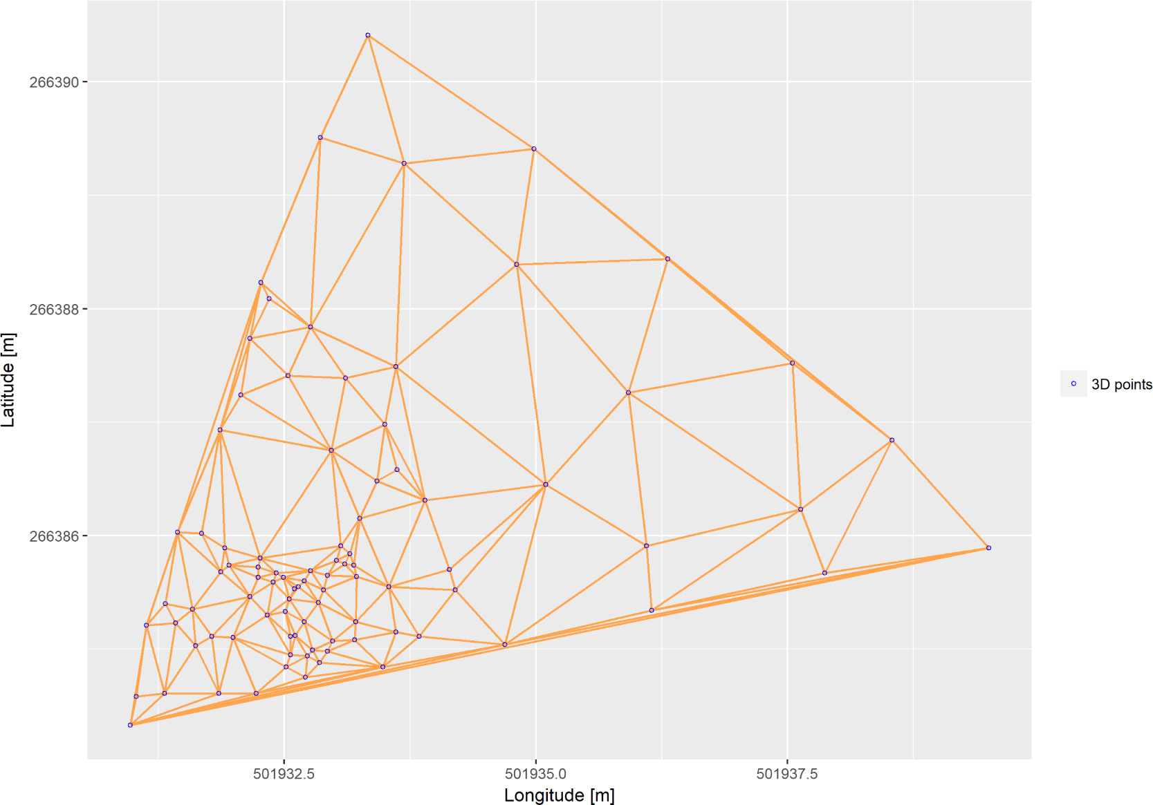   Figure 2

   Delaunay triangulation of the investigated points; ETRS89 (EPSG 2180) coordinate reference system was used

   

   Figure 3

   Relationship between collinearity and dip angle for Delaunay triangles

   

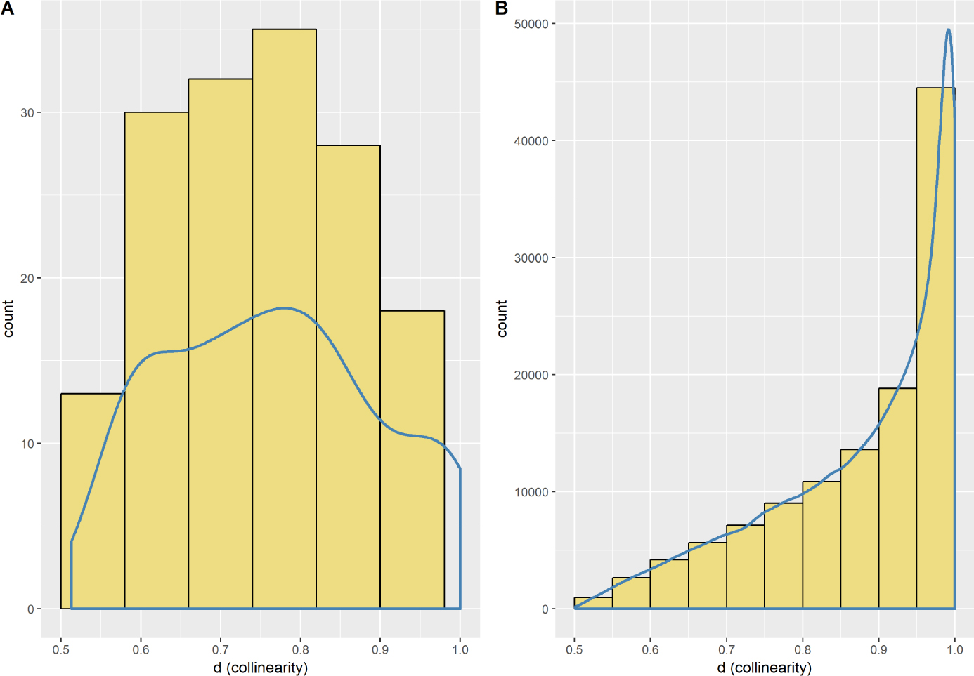   Figure 4

   The distribution of collinearity (A) Collinearity attributed to Delaunay triangles (B) Collinearity attributed to 117 480 planes generated by Lipski algorithm

   Because our goal was to estimate the maximum possible value of collinearity, we generated all three-element subsets from the ninety-element set. This was achieved using an algorithm of generating k-element subsets from an n-element set [26]. According to the well-known binomial coefficient we obtained 117 480 planes. Because the distribution plot indicates the prevalence of collinear planes (Figure 4B), we can investigate closer the relationship between the collinearity, size (expressed in m²) and the orientation parameters in further steps.

3 Results

We extended the initial set of measurements by using the combinatorial algorithm and obtained the relationship between collinearity, size and the dip angle (Figure 5A). We included also certain partial plots that describe this relationship in smaller intervals. The dip angle had relatively lower dispersion (about 12-15 degrees) among equilateral triangles. This dispersion can be significantly reduced (to approximately 1-3 degrees) when considering only the greatest planes (Figure 5B). The visual effect of these results can be described as follows: the greatest planes had warm (yellow-red) colours and formed a relatively narrow belt. This belt was surrounded from both sides by planes of smaller size that can be recognized by their cooler colours. This effect did not happen on the other side of the considered interval of collinearity. When considering more collinear configurations, we observed greater randomness of the dip angle (Figure 5C). However, even for the interval [0.99750, 1] we could still recognize the narrow belt representing the expected value of the dip angle. The loss of the ability of recognizing this value can be observed for planes whose collinearity is greater than approximately 0.9999 (Figure 5D).

Figure 5

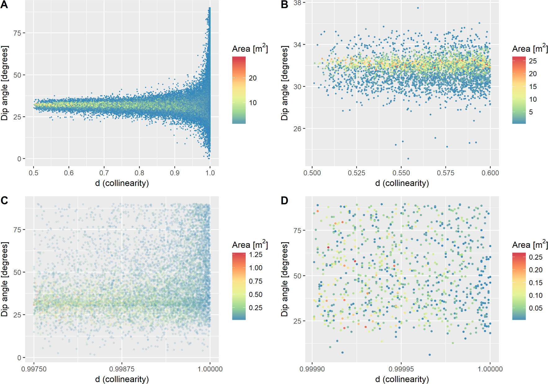
Relationship between collinearity, size and dip angle for 117 480 planes (A) The entire interval of collinearity is considered (B) Equilateral configurations are examined (0.5<d <0.6) (C) The interval for almost collinear triangles is considered (d>0.9975) (D) Even more collinear configurations are presented (d>0.9999)

Thus, taking into consideration all measurements would have affected the distribution, especially the measures of dispersion (Figure 6A). The practical results of this study can be referred to improving the quality of the initial distribution of the dip angle generated by Delaunay triangulation. We suggested observing distributions of the dip angle with respect to the increasing degree of collinearity. We avoided establishing new arbitrary coefficients of universal significance. But because the examined surface was relatively uniformly oriented, it was straightforward to estimate the interval at which outliers began to affect the distribution (Figure 3, Figure 6A). We considered a conditional distribution and obtained the anticipated results: the median has generally not changed; a small change is to observe for the mean value but the most significant change happened to the standard deviation (Figure 6A, Figure 6B).

Figure 6

(A) The distribution of the dip angle for all Delaunay triangles (B) A conditional distribution of the dip angle for Delaunay triangles whose d is smaller than 0.975

4 Discussion

In this article we investigated the impact of collinearity on the reliability of measurements of the attitude of geological planes. Previous studies addressing this issue referred to a measure based on eigenvalues of the “orientation matrix” and certain limitations were suggested. This approach, however, refers more to the spatial distribution of points rather than to configuration of local planes whose attitude is investigated. Moreover, the inaccuracies of the floating-point arithmetic were not considered as a source of potential errors. The main goal of this study was to supply a more intuitive measure of collinearity that covers its whole interval of variability. This allowed to examine the impact of this feature on the numerical stability of the output data. However, the impression of arbitrariness will probably be always present when putting numerical restrictions on the input data. Nevertheless, to detect outliers, we suggested a criterion that refers more to the case-by-case approach based on observing the distribution of the measured parameter. The above approach can be applied as long as the surface is uniformly oriented or its orientation is known a priori so that the outliers can be easily detected. In our study we examined the orientation of a uniformly oriented surface that was locally approximated by planes generated by the Delaunay triangulation. The main goal of this approach differed from this that was considered in the best-fitting method. The key problem was not to compute the dip angle and the dip direction but to find measurements affected by rounding errors of the floating-point arithmetic. We showed that collinearity influences the dip angle (e.g., Figure 3, Figure 5A, Figure 6A) but because of the small number of measurements we were not able to describe the relationship between selected parameters. In order to investigate it, we used a combinatorial algorithm, that supplied a greater number of planes affected by collinearity. Figure 5B shows that the smallest deviation from the expected value can be attributed to the greatest planes. Moreover, the small planes of equilateral shape did not influence the dip angle as much as collinear planes of relatively greater size (Figure 5B, Figure 5D). A non-intuitive conclusion from this study is that the distribution of collinearity within a considered set of points can be far from symmetric (Figure 4B) although triangles of different shapes were considered. We do not regard this asymmetric result as a general rule when investigating all possible planes within a considered dataset. Nevertheless, this example shows that selecting at random sample planes from a dataset and computing the average orientation may lead to unexpected results. This is because in our case the probability of selecting a collinear plane at random was relatively high but we indicated that the collinear configurations are not reliable in terms of obtaining the attitude. Thus, considering Delaunay triangulation seems to be a partial solution to this problem. Nevertheless, to reduce the dispersion of the measurements obtained by the Delaunay triangulation, we suggested a restriction. In our case we selected the biggest subset which does not include any outliers. Thus, we reduced the interval of acceptable collinearity (Figure 6B). In our case we set the threshold of collinearity to 0.975 but we do not assume that this value should be used in all circumstances. Because great dispersion of data is often treated as a drawback behind a considered approach, our results should improve the reliability of obtaining the measurements of attitude in similar geological and methodological circumstances.

References

[1] Fienen M. N., The Three-Point Problem, Vector Analysis and Extension to the N-Point Problem. Journal of Geoscience Education, 2005, 53, 257–6310.5408/1089-9995-53.3.257Suche in Google Scholar
[2] De Paor D.G., A Modern Solution to the Classical Three-Point Problem. Journal of Geological Education, 1991, 1, 322–2410.5408/0022-1368-39.4.322Suche in Google Scholar
[3] Vacher H. L., The Three-Point Problem in the Context of Elementary Vector Analysis. Journal of Geological Education, 1989, 8, 280–8710.5408/0022-1368-37.4.280Suche in Google Scholar
[4] Haneberg W. C., A Lagrangian interpolation method for three-point problems. Journal of Structural Geology, 1990, 12, 945-947, https://doi.org/10.1016/0191-8141(90)90069-B10.1016/0191-8141(90)90069-BSuche in Google Scholar
[5] Ragan D. M., Structural Geology: An Introduction to Geometrical Techniques. Cambridge University Press, 200910.1017/CBO9780511816109Suche in Google Scholar
[6] Groshong R. H., 3-D Structural Geology. Springer-Verlag Berlin Heidelberg, 200610.1007/978-3-540-31055-6Suche in Google Scholar
[7] Feng Q., Sjögren P., Stephansson O., Jing L., Measuring fracture orientation at exposed rock faces by using a non-reflector total station. Eng. Geol., 2001, 59, 133-146, https://dol.org/10.1016/S0013-7952(00)00070-310.1016/S0013-7952(00)00070-3Suche in Google Scholar
[8] Xu X., Bhattacharya J. B., Davies R. K., Aiken C. L., Digital geologic mapping of the Ferron Sandstone, Muddy Creek, Utah, with GPS and reflectorless laser rangefinders. GPS Solutions, 2001, 5, 15-23, https://doi.org/10.1007/PL0001287210.1007/PL00012872Suche in Google Scholar
[9] Cracknell M. J., Roach M., Green D., Lucieer A., Estimating bedding orientation from high-resolution digital elevation models. IEEE Transactions on Geoscience and Remote Sensing, 2013, 51, 2949-2959, https://doi.org/10.1109/TGRS.2012.221750210.1109/TGRS.2012.2217502Suche in Google Scholar
[10] Banerjee S., Mitra S., Remote surface mapping using orthophotos and geologic maps draped over digital elevation models: Application to the Sheep Mountain anticline, Wyoming. AAPG bulletin, 2004, 88, 1227-123710.1306/02170403091Suche in Google Scholar
[11] Martinez-Torres L. M., Lopetegui A., Eguiluz L., Automatic resolution of the three-points geological problem. Computers & Geosciences, 2012, 42, 200-202, https://doi.org/10.1016/j.cageo.2011.08.03110.1016/j.cageo.2011.08.031Suche in Google Scholar
[12] Hasbargen L. E., A test of the three-point vector method to determine strike and dip utilizing digital aerial imagery and topography. Geological Society of America Special Papers, 2012, 492, 199-208, http://dx.doi.org/10.1130/2012.2492(14)10.1130/2012.2492(14)Suche in Google Scholar
[13] McCaffrey K. J. W., Jones R. R., Holdsworth R. E., Wilson R. W., Clegg P., Imber J., Holliman N., Trinks I., Unlocking the spatial dimension: digital technologies and the future of geoscience fieldwork. Journal of the Geological Society, 2005, 162, 927-938, https://doi.org/10.1144/0016-764905-01710.1144/0016-764905-017Suche in Google Scholar
[14] Bistacchi A., Griffith W. A., Smith S. A., Di Toro G., Jones R., Nielsen S., Fault roughness at seismogenic depths from LIDAR and photogrammetric analysis. Pure and Applied Geophysics, 2011, 168, 2345-2363, https://doi.org/10.1007/s00024-011-0301-710.1007/s00024-011-0301-7Suche in Google Scholar
[15] Assali P., Grussenmeyer P., Villemin T., Pollet N., Viguier F., Solid images for geostructural mapping and key block modeling of rock discontinuities. Computers & Geosciences, 2016, 89, 21-31, https://doi.org/10.1016/j.cageo.2016.01.00210.1016/j.cageo.2016.01.002Suche in Google Scholar
[16] Dewez T. J., Girardeau-Montaut D., Allanic C., Rohmer J., Facets: A CloudCompare plugin to extract geological planes from unstructured 3D point clouds. International Archives of the Photogrammetry, Remote Sensing & Spatial Information Sciences, 2016, 41, 799-804, https://doi.org/10.5194/isprs-archives-XLI-B5-799-201610.5194/isprs-archives-XLI-B5-799-2016Suche in Google Scholar
[17] Scheidegger A. E., On the statistics of the orientation of bedding planes, grain axes, and similar sedimentological data. US Geological Survey Professional Paper, 1965, 525, 164-167Suche in Google Scholar
[18] Watson G. S., Equatorial distributions on a sphere. Biometrika, 1965, 52, 193-201, https://doi.org/10.1093/biomet/52.1-2.19310.1093/biomet/52.1-2.193Suche in Google Scholar
[19] Woodcock N. H., Specification of fabric shapes using an eigenvalue method. Geological Society of America Bulletin, 1977, 88, 1231-1236, https://doi.org/10.1130/0016-7606(1977)88%3C1231:SOFSUA%3E2.0.CO;210.1130/0016-7606(1977)88<1231:SOFSUA>2.0.CO;2Suche in Google Scholar
[20] Fernández O., Obtaining a Best Fitting Plane through 3D Georeferenced Data. Journal of Structural Geology, 2005, 27, 855–58, https://doi.org/10.1016/j.jsg.2004.12.00410.1016/j.jsg.2004.12.004Suche in Google Scholar
[21] Jones R. R., Pearce M. A., Jacquemyn C., Watson F. E., Robust best-fit planes from geospatial data. Geosphere, 2016, 12, 196-202, https://doi.org/10.1130/GES01247.110.1130/GES01247.1Suche in Google Scholar
[22] Goldberg D., What every computer scientist should know about floating-point arithmetic. ACM Computing Surveys (CSUR), 1991, 23, 5-48, https://doi.org/10.1145/103162.10316310.1145/103162.103163Suche in Google Scholar
[23] Mei G., Tipper J. C., Xu N., Numerical robustness in geometric computation: An expository summary. Applied Mathematics & Information Sciences, 2014, 8, 2717, http://dx.doi.org/10.12785/amis/08060710.12785/amis/080607Suche in Google Scholar
[24] Seers T. D., Hodgetts D., Probabilistic constraints on structural lineament best fit plane precision obtained through numerical analysis. Journal of Structural Geology, 2016, 82, 37-47, https://doi.org/10.1016/j.jsg.2015.11.00410.1016/j.jsg.2015.11.004Suche in Google Scholar
[25] de Berg M., Cheong O., van Kreveld M., Overmars M., Computational Geometry. Springer-Verlag Berlin Heidelberg, Berlin, Heidelberg, 200810.1007/978-3-540-77974-2Suche in Google Scholar
[26] Lipski W., Combinatorics for programmers. Wydawnictwa Naukowo-Techniczne, Warsaw, 2004Suche in Google Scholar
[27] Hert S., Seel M., dD Convex Hulls and Delaunay Triangulations. In: CGAL User and Reference Manual. CGAL Editorial Board, 4.13 edition, 2018. <http://www.cgal.org/Manual/>Suche in Google Scholar
[28] Fogel E., Halperin D., Wein R., CGAL arrangements and their applications: A step-by-step guide. Springer Science & Business Media, 2012, http://dx.doi.org/10.1007/978-3-642-17283-010.1007/978-3-642-17283-0Suche in Google Scholar
© 2018 M. Michalak, published by De Gruyter.
This work is licensed under the Creative Commons Attribution-NonCommercial-NoDerivatives 4.0 License.
Artikel in diesem Heft
- Regular Articles
- Spatio-temporal monitoring of vegetation phenology in the dry sub-humid region of Nigeria using time series of AVHRR NDVI and TAMSAT datasets
- Water Quality, Sediment Characteristics and Benthic Status of the Razim-Sinoie Lagoon System, Romania
- Provenance analysis of the Late Triassic Yichuan Basin: constraints from zircon U-Pb geochronology
- Historical Delineation of Landscape Units Using Physical Geographic Characteristics and Land Use/Cover Change
- ‘Hardcastle Hollows’ in loess landforms: Closed depressions in aeolian landscapes – in a geoheritage context
- Geostatistical screening of flood events in the groundwater levels of the diverted inner delta of the Danube River: implications for river bed clogging
- Utilizing Integrated Prediction Error Filter Analysis (INPEFA) to divide base-level cycle of fan-deltas: A case study of the Triassic Baikouquan Formation in Mabei Slope Area, Mahu Depression, Junggar Basin, China
- Architecture and reservoir quality of low-permeable Eocene lacustrine turbidite sandstone from the Dongying Depression, East China
- Flow units classification for geostatisitical three-dimensional modeling of a non-marine sandstone reservoir: A case study from the Paleocene Funing Formation of the Gaoji Oilfield, east China
- Umbrisols at Lower Altitudes, Case Study from Borská lowland (Slovakia)
- Modelling habitats in karst landscape by integrating remote sensing and topography data
- Mineral Constituents and Kaolinite Crystallinity of the <2 μm Fraction of Cretaceous-Paleogene/Neogene Kaolins from Eastern Dahomey and Niger Delta Basins, Nigeria
- Construction of a dynamic arrival time coverage map for emergency medical services
- Characterizing Seismo-stratigraphic and Structural Framework of Late Cretaceous-Recent succession of offshore Indus Pakistan
- Geosite Assessment Using Three Different Methods; a Comparative Study of the Krupaja and the Žagubica Springs – Hydrological Heritage of Serbia
- Use of discriminated nondimensionalization in the search of universal solutions for 2-D rectangular and cylindrical consolidation problems
- Trying to underline geotourist profile of National park visitors: Case study of NP Fruška Gora, Serbia (Typology of potential geotourists at NP Fruška Gora)
- Fluid-rock interaction and dissolution of feldspar in the Upper Triassic Xujiahe tight sandstone, western Sichuan Basin, China
- Calcified microorganisms bloom in Furongian of the North China Platform: Evidence from Microbialitic-Bioherm in Qijiayu Section, Hebei
- Spatial predictive modeling of prehistoric sites in the Bohemian-Moravian Highlands based on graph similarity analysis
- Geotourism starts with accessible information: the Internet as a promotional tool for the georesources of Lower Silesia
- Models for evaluating craters morphology, relation of indentation hardness and uniaxial compressive strength via a flat-end indenter
- Geotourism in an urban space?
- The first loess map and related topics: contributions by twenty significant women loess scholars
- Modeling of stringer deformation and displacement in Ara salt after the end of salt tectonics
- A multi-criteria decision analysis with special reference to loess and archaeological sites in Serbia (Could geosciences and archaeology cohabitate?)
- Speleotourism in Slovenia: balancing between mass tourism and geoheritage protection
- Attractiveness of protected areas for geotourism purposes from the perspective of visitors: the example of Babiogórski National Park (Poland)
- Implementation of Heat Maps in Geographical Information System – Exploratory Study on Traffic Accident Data
- Mapping War Geoheritage: Recognising Geomorphological Traces of War